Phase Diagram of Vortices in High-${\bf T_{c}}$ Superconductors from Lattice Defect Model with Pinning

Abstract

The theory presented is based on a simple Hamiltonian for a vortex lattice in a weak impurity background which includes linear elasticity and plasticity, the latter in the form of integer valued fields accounting for defects. Within a quadratic approximation in the impurity potential, we find a first-order Bragg-glass, vortex-glass transition line showing a reentrant behavior for superconductors with a melting line near $H_{c2}$. Going beyond the quadratic approximation by using the variational approach of Mézard and Parisi established for random manifolds, we obtain a phase diagram containing a third-order glass transition line. The glass transition line separates the vortex glass and the vortex liquid. Furthermore, we find a unified first-order line consisting of the melting transition between the Bragg glass and the vortex liquid phase as well as a disorder induced first-order line between the Bragg glass and the vortex glass phase. The reentrant behavior of this line within the quadratic approach mentioned above vanished. We calculate the entropy and magnetic induction jumps over the first-order line.

I Introduction

The phase diagram of high-$T_{c}$ superconductors in the $H-T$-plane is dominated by the interplay of thermal fluctuations and disorder Blatter1 ; Nattermann1 . It is believed that at low magnetic fields near $T_{c}$ the vortex solid melts into a vortex liquid (VL) via a first-order melting transition. Prominent examples of high-$T_{c}$ superconductors exhibiting a solid-liquid melting are the anisotropic compound ${\rm YBa}_{2}{\rm Cu}_{3}{\rm O}_{7-\delta}$ (YBCO), and the strongly layered compound ${\rm Bi}_{2}{\rm Sr}_{2}{\rm Ca}{\rm Cu}_{2}{\rm O}_{8}$ (BSCCO). When including weak pinning, the solid phase becomes a quasi-long-range ordered Bragg glass (BG) Blatter1 . At higher magnetic fields, the quasi-long-range order is destroyed and there exist also a vortex glass (VG) phase. The transition is marked by the disappearance of Bragg peaks in scattering data. There is strong experimental evidence especially for BSCCO Avraham1 ; Beek1 but also for YBCO Radzyner1 that the BG-VG transition is first order, although in YBCO it has not been confirmed that this is really a proper phase transition, not just a crossover. So far, the transition line has been identified only by some magnetic anomalies in the response to the external magnetic field.

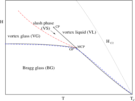
Figure 1: Sketch of the two possible scenarios of the phase diagram of YBCO or similar high-$T_{c}$ superconductors where the phase transition line lies near $H_{c2}$. The straight line corresponds to the BG-VG, BG-VL first-order lines with an extension of the first-order line beyond the lower multicritical point (MCP). This is the first scenario discussed in the text. The dashed line corresponds to a unified BG-VG, BG-VL first-order line without a slush phase (VS) corresponding to the second scenario. The dashed-dotted line is the glass transition line. The point GP is the intersection point of the glass transition line with the BG-VG, BG-VL line.

For BSCCO it seems that the two melting lines are part of a unified first-order transition line. For YBCO there are two possible experimental scenarios: First, the BG-VG and the BG-VL transition lines meet in a multicritical point (MCP) Bouquet1 where the thermodynamical character of the BG-VG line is not clear. The first-order BG-VL melting line should continue beyond the multicritical point ending in a critical point (CP) Pal1 ; Shibata1 where a new fluid-like phase, the slush phase (VS), emerges (see Fig. 1).

The second scenario consists of a unified melting line Radzyner1 without a multicritical point which is the case for BSCCO. We note that the experimentally realized scenario is strongly sensitive on the doping of the superconductor Shibata1 .

Beside the first-order transition lines, there exits a glass transition line between the VG and VS phases, if the VS phase exists, or between the VG and VL phases, if VS is absent. This glass transition line was predicted by Fisher et al. in Ref. Fisher1, , and observed when confirming scaling rules for special current-voltage characteristics across the transition line Gammel1 . Alternatively it was proposed in Ref. Reichhardt1, that the glass transition is window glass like with no scaling. Some people define an irreversibility line beyond which magnetization sweeps are no longer reversible Nishizaki1 . This seems to coincide with the glass transition line. A direct experimental determination of the order of the glass transition in the vortex system of YBCO has not yet been possible. For BSCCO, there is recent experimental evidence that the glass transition line could be of second order Beidenkopf1 . A sketch of the phase diagram for YBCO which contains the two scenarios is shown in Fig. 1.

Beside experiments to determine the phase diagram, information comes from computer simulations based on the Langevin equation Otterlo1 or on frustrated XY-models Nonomura1 ; Olsson1 ; Rodriguez1 . The Langevin simulations confirm the second phase scenario without a slush phase, and the existence of a multicritical point on the melting line being unclear. In the frustrated XY model, the existence of a slush phase and of a multicritical point are also controversial Olsson2 . In addition, Lidmar Lidmar1 carried out a Monte-Carlo simulation based on a defect model where he only obtains a first-order melting line and a glass transition line, but not a VS phase.

Analytic approaches are based mainly on the Ginzburg Landau model Li1 , which is especially useful for YBCO, the cage model Ertas1 , or the elasticity model of the vortex lattice Giamarchi2 ; Mikitik1 ; Mikitik2 ; Kierfeld1 ; Kierfeld2 ; Radzyner2 ; Menon1 with pinning. The Ginzburg Landau model with pinning was analyzed recently by Li et al. Li1 where they found a phase diagram of the second scenario, with a single first-order melting line between the VG and VL phases as well as between the BG and VG phases, without an additional slush phase. The calculation was restricted to second order in the disorder potential. In a recent paper they also carry out an analysis of a possible glass transition line in the fluid phase of the Ginzburg-Landau model where they found such a line only under a certain disorder model Li2 by using replica symmetry-breaking techniques which we also use in this paper. In Ertas1 ; Giamarchi2 ; Mikitik1 ; Menon1 ; Radzyner2 ; Kierfeld2 the phenomenological Lindemann criterion extended to include pinning was used in order to calculate the BG-VG and BG-VL transition lines. In Kierfeld1 ; Mikitik2 defects were taken into account for determining the transition lines. These approaches allow for an explanation of both phase scenarios.

It is the purpose of this paper to investigate the above phase transitions in a defect melting model which was recently constructed for the study of defect-induced melting of square (YBCO) and triangular (BSCCO) vortex lattices. The model is a modification of a simpler version in Ref. GFCM2, which explained the melting transition of ordinary crystals by the statistical mechanics of defects on a hypothetical square lattice. This model was generalized for two-dimensional triangular crystals in Ref. Dietel1, . The model is Gaussian in the elastic strains and takes into account the defect degrees of freedom by integer valued gauge fields. The melting line is found from a lowest-order approximation, in which one identifies the melting point with the intersection of the high-temperature expansion of the free energy density dominated by defect fluctuations with the low-temperature expansion dominated by elastic fluctuations.

In this paper we shall consider, in addition, the effect of weak disorder on the melting line near $H_{c2}$. This will lead to a determination of the BG-VG and BG-VL transition line. The most prominent example for a high-$T_{c}$ superconductors with such a melting line is YBCO but also superconductors with a low critical temperature $T_{c}$ such as BCS type superconductors or with a small anisotropy factor should have a melting line near $H_{c2}$. For concrete calculations, we will restrict us in the following to the case of YBCO.

The paper will first review the model and derive an effective Hamiltonian for the vortex lattice in the low-temperature solid phase and the high-temperature fluid phase without disorder. The model has two mutually representations. One can be evaluated efficiently in the low-temperature phase, the other in the high-temperature phase. The lowest approximation to the former contains only elastic fluctuations of the vortex lattice without defects. The dual representation sums over all integer-valued stress configurations, which to lowest approximation are completely frozen out. The tranverse part of the vortex fluctuations in the high-temperature approximation corresponds to non-interacting three-dimensional elastic strings where the length in z-direction is discretized with the dislocation length as the lattice spacing Dietel2 . It is well known, that the lower critical dimension for an elastic string in a random potential Halpin1 is three. This dimension separates the string system in higher dimensions with two phases (a disorder dominated low-temperature phase and a temperature dominated high-temperature phase) from a single disorder dominated phase in lower dimensions. We encounter a similar situation for the high temperature Hamiltonian in Sect. V. This is the reason, why we shall have to consider higher-order expansion terms Gorokhov1 .

We shall first expand the free energy to lowest order in the disorder potential in Section III. The result will be a unified melting line. This line bends to lower magnetic fields in the direction for decreasing temperatures due to the disorder, in agreement with experiments. We obtain a remarkable reentrant behavior for this line. We do not obtain, however, a good agreement with experiments at low magnetic fields. In order to get better agreement with experiment and to determine also the glass transition line we further calculate, in the solid low-temperature phase and in the fluid high-temperature phase, the free energy non-perturbatively by using once the replica-trick and further the variational approach set up by Mézard and Parisi Mezard1 for random manifolds and spin-glasses Dotsenko1 . It is based on replacing the non-quadratic part of the replicated Hamiltonian by quadratic one, with possible mixing of replica fields. A transition line from a liquid to a glass consists within the Mézard-Parisi approach on a boundary in thermodynamical space from a replica symmetric quadratic Hamiltonian to a Hamiltonian which breaks the symmetry in the replica fields. The best quadratic Hamiltonian in the low-temperature solid phase is full replica symmetry broken corresponding to the BG-phase. In the high-temperature phase we find a region where the solution is full replica symmetric corresponding to the VL phase. Furthermore, we find a glassy region (VG) were the optimal quadratic Hamiltonian depends on the form of the disorder correlation function. By carrying a comprehensive stability analysis in Section VII we show that for the form of the glassy state the kurtosis $\kappa_{1}$ defined in (87) as functional on the positional disorder function is relevant. A Gaussian correlation function has kurtosis $\kappa_{1}=1$. For high magnetic fields near $H_{c2}$ we obtain:
For $\kappa_{1}<1$ we get a one-step replica symmetry broken solution with a third-order phase transition line. This corresponds to a correlation function with flatter tip and smaller tail than the Gaussian correlation function. In the case $\kappa_{1}\geq 1$ we obtain a full replica symmetry broken solution. The free energy has the same form as in the one-step replica symmetry breaking case leading also to a third-order glass transition line. Disorder correlation functions with smaller tips and larger tails than the Gaussian correlation function belong to this case. For lower magnetic fields we obtain that the border in the disorder function space of one-step and continous replica symmetry broken solutions moves to lower kurtosis.

The VG-VL phase transition happens just at the depinning temperature of a one-dimensional string in three dimensions subjected to impurities Blatter1 . We calculate the free energies in the low-temperature solid and in both high-temperature phases. By the intersection criterion we obtain further the first-order BG-VL and BG-VG transition line. We do not find an additional first-order line which separates the slush phase VS from the vortex liquid VL. Summarizing, we obtain within our approach only the second scenario. In the low-temperature solid phase our analysis corresponds to the analysis of Korshunov Korshunov1 and Giamarchi and Doussal Giamarchi1 using the Mézard-Parisi approach for the vortex lattice system in random potentials. Because this system does not contain defects only the Bragg glass phase can be described correctly. Within our approach we include beside the disorder ones also the defect degrees of freedom by integer valued fields which are important to obtain the melting transition. This allows us to compute the whole phase diagram for YBCO. In this sense our theory is a direct generalization of the earlier vortex lattice approaches in random potentials.

Beside the results above, we give in Appendix B a derivation of some stability theorems of saddle point solutions similar to the theorems of Carlucci et al. Carlucci1 derived within the large $N^{\prime}$-limit approach of Mézard and Parisi Mezard1 where $N^{\prime}$ are the number of components of the random manifold. Because in general the number of components of a given random manifold is rather small it is useful to generalize these theorems also to the variational approach of Mezard-Parisi not existent in literature yet.

The paper is organized as follows:
In Section II we state the model of the vortex lattice with defects and impurity degrees of freedoms. We derive in Section III the effective low and high-temperature Hamiltonian of the vortex lattice without impurities. With the help of these effective Hamiltonians we calculate in Section IV the BG-VG, BG-VL transition line within the second order perturbation theory in the disorder potential. In Section V we introduce the Mézard-Parisi variational approach. Section VI calculates the saddle point solutions of the self-energy matrices for the variational free energy within the Mézard-Parisi approach in the fluid high-temperature phase. Section VII deals with the stability of the calculated saddle-point solutions. Section VIII calculates the saddle point solutions in the solid phase. In Section IX, we discuss the phase diagram of the Mézard-Parisi approach for YBCO and compare it with the experimental ones. Furthermore jump quantities are calculated in this section. Section X contains a summary of the paper.

II Model

The partition function used here for the vortex lattice without disorder was proposed in Ref. Dietel2, . It is motivated by similar melting models for two-dimensional square GFCM2 and triangular Dietel1 crystals. Motivated by the fact that YBCO has a square vortex lattice we restrict us here to a discussion of the phase diagram of such type of lattice. The generalization to triangular vortex lattices is straight forward Dietel2 resulting only in a slight difference in numerical values. We briefly summarize the important features of the model. The partition function of the disordered flux line lattice can be written in the canonical form as a functional integral

$$Z_{\rm fl}\!=\!\int{\cal D}[u_{i},\sigma_{im},n_{i}]e^{-\left(H_{0}[u_{i},\sigma_{im},n_{i}]+H_{\rm dis}[u_{i}]\right)/k_{B}T}\,,$$ (1)

where

$$\frac{H_{0}[u_{i},\sigma_{im},n_{i}]}{k_{B}T}=\sum_{{\bf x}}\frac{1}{2\beta}\Bigg{[}\sum_{i<j}\sigma_{ij}^{2}+\frac{1}{2}\sum_{i}\sigma_{ii}^{2}-\Big{(}\!\sum_{i}\frac{\overline{\nabla}_{i}}{\nabla_{i}}\sigma_{ii}\!\Big{)}\frac{c_{11}-2c_{66}}{4(c_{11}-c_{66})}\Big{(}\!\sum_{i}\frac{\overline{\nabla}_{i}}{\nabla_{i}}\sigma_{ii}\!\Big{)}+\sum_{i}\sigma_{i3}\frac{c_{66}}{c_{44}}\sigma_{i3}\Bigg{]}$$

$$-2\pi i\sum_{{\bf x}}\left(\sum_{i,m}\sigma_{im}\nabla_{m}u_{i}+\sum_{i\leq j}\sigma_{ij}N_{ij}\right)$$ (2)

is the canonical representation of elastic and plastic energies summed over the lattice sites ${\bf x}$ of a three-dimensional lattice, and $\sigma_{ij}$ where $\sigma_{21}\equiv\sigma_{12}$ are stress fields which are canonically conjugate to the distortion fields GFCM2 . The subscripts $i,j$ have the values $1,2$, and $l,m,n$ run from $1$ to $3$. The parameter $\beta$ is proportional to the inverse temperature, $\beta\equiv a^{2}a_{3}c_{66}/k_{B}T(2\pi)^{2}$, where $a$ is the transverse distance of neighboring vortex lines, and $a_{3}$ is the persistence length along the dislocation lines introduced in Ref. Dietel2, . Note that $a_{3}$ is assumed to be independent on the disorder potential on the average. The volume of the fundamental cell $v$ is equal to $a^{2}a_{3}$ for the square lattice.

The matrix $N_{ij}({\bf x})$ in Eq. (5) is a discrete-valued local defect matrix composed of integer-valued defect gauge fields $n_{1},n_{2}$. It depends on the lattice symmetry Dietel1 . For a square vortex lattice it is given by

$$N_{ij}\!\! = \!\!\left(\begin{array}[]{cr}n_{1}&n_{2}\\ n_{2}&-n_{1}\end{array}\right).$$ (5)

The lattice derivatives $\nabla_{m}$ and their conjugate counterparts $\overline{\nabla}_{m}$ are the lattice differences for a cubic three-dimensional crystal. In the xy-plane they are defined by

$$\nabla_{i}f({\bf x}) \equiv [f({\bf x})-f({\bf x}-a{\bf e}_{i})]/a,$$

$$~{}~{}\overline{\nabla}_{i}f({\bf x}) \equiv [f({\bf x}+a{\bf e}_{i})-f({\bf x})]/a$$ (6)

for a lattice function $f({\bf x})$, where ${\bf e}_{i}$ are unit vectors to the nearest neighbors in the plane. The corresponding derivatives in $z$-direction are defined similarly. We have suppressed the spatial arguments of the elasticity parameters, which are functional matrices $c_{ij}({\bf x},{\bf x}^{\prime})\equiv c_{ij}({\bf x}-{\bf x}^{\prime})$. Their precise forms were first calculated by Brandt Brandt1 and generalized in Ref. Dietel2 by taking into account thermal softening relevant for BSCCO.

The second term in the exponent of (1)

$$H_{\rm dis}[u_{i}]=\sum_{{\bf x}}V({\bf x}+{\bf u}),$$ (7)

accounts for disorder. The measure of the functional integral is

$$\!\!\!\!\!\!\!\!\!\!\!\!\!\!\!\!\!\!\!\!\int{\cal D}[u_{i},\sigma_{im},n_{i}]\!=\!\rm{det}\left[\frac{c_{66}}{4(c_{11}\!-\!c_{66})}\right]^{1/2}\!\!\!\!\!\rm{det}\left[\frac{1}{2\pi\beta}\right]^{5/2}~{}~{}~{}~{}~{}~{}$$

$$~{}~{}\times\!\left\{\!\prod_{{\bf x}}\!\Bigg{[}\prod_{i\leq m}\int_{-\infty}^{\infty}d\sigma_{im}\!\Bigg{]}\Bigg{[}\!\prod_{j}\sum_{n_{j}({\bf x})=-\infty}^{\infty}\Bigg{]}\Bigg{[}\!\int_{-\infty}^{\infty}\frac{d{\bf u}}{a}\Bigg{]}\!\right\}.~{}$$ (8)

The disorder potential $V({\bf x})$ due to pinning is assumed to possess the Gaussian short-scale correlation function

$$\overline{V({\bf x})V({\bf x}^{\prime})} = \Delta(x_{i}-x_{i}^{\prime})\delta_{x_{3},x_{3}^{\prime}}$$

$$= d(T)\,a_{3}\,\frac{\phi_{0}^{4}\,\xi^{3}_{ab}}{\tilde{\lambda}_{ab}^{4}}K(x_{i}-x_{i}^{\prime})\,\delta_{x_{3},x_{3}^{\prime}}$$

where $K(x_{i}-x_{i}^{\prime})\approx 1/(\xi^{\prime})^{2}$ for $|{\bf x}-{\bf x}^{\prime}|<\xi^{\prime}$, and is zero elsewhere, and $\phi_{0}$ is the magnetic flux quantum $\phi_{0}=hc/2e$. The parameter $\xi^{\prime}$ is the correlation length of the impurity potential which is similar to the coherence length $\xi_{ab}$ in the $xy$-plane. $\tilde{\lambda}_{ab}=\lambda_{ab}/(1-b)$ is the screened penetration depth in the $xy$-plane Mikitik1 .

The temperature dependence of the parameter $d(T)$ is mainly due to the temperature dependence of the correlation length and the pinning mechanism where we discuss in the following the $\delta T_{c}$-pinning or $\delta_{l}$-pinning mechanisms Blatter1 .

Both pinning mechanisms are extensively discussed in the review of Blatter et al. Blatter1 . We just mention that the $\delta T_{c}$-pinning mechanism has its origin in fluctuations in $T_{c}$ in the Ginzburg-Landau free energy and the $\delta l$-pinning mechanism is due to fluctuations in the mean free path coming from fluctuations in the impurity density. The parameter $d(T)$ is different for both pinning mechanisms Blatter1 :

$$d(T) = d_{0}(1-T/T_{C})^{-1/2}\quad{\rm for}\quad\delta T_{c}-{\rm pinning}\,,$$ (10)

$$d(T) = d_{0}(1-T/T_{C})^{3/2}\quad\;\;{\rm for}\quad\delta l-{\rm pinning}.$$ (11)

The correlation functions for both mechanisms can be derived in Fourier space by taking into account the order parameter shape of a single vortex Blatter1 . This is of long range, resulting in a divergence of the Fourier transformed disorder correlation function $\hat{K}(q)$ at $q=0$ for the $\delta T_{c}$-pinning mechanism. This divergence is regulated for a vortex in a lattice by omitting the regime $q\lesssim 1/a$ because the order parameter of the superposition of non-cut off single vortex order parameters on the lattice would otherwise scale with the system size. We shall see below in Section VII that this is the momentum region of the disorder correlation function which determines mainly the form of the free energy in the fluid phase near the glass transition line and thus the order of the glass transition. Other correlation mechanism as for example screening of impurities are not taken into account in these single vortex disorder correlation functions. The screening of impurity potentials is important because the nearest neighbor distance between impurities is typically of the same size as the coherence length $\xi_{ab}$ Blatter1 .

All this leads us to use in the calculations to follow an effective disorder correlation function with the Fourier transform

$${\hat{K}}(q)=2\pi\exp(-{\xi^{\prime}}^{2}q_{i}^{2}/2)\qquad$$ (12)

leading also to an exponentially vanishing of the disorder correlation function in real space. The advantage for using this effective correlation function is that one gets simple analytical formulas in the calculations. The parameter $\xi^{\prime}$ in (12) is an effective correlation length which can also include for example screening effects of the impurities in the $\delta_{l}$-pinning case. The approximation (12) leads to well known approximations for the temperature softening of quantities which use the disorder correlation functions as an input as for example the temperature softening of the coherently time-averaged pinning energies Blatter1 .

In the following sections, we come back to the more general case without the assumption (12) for the disorder correlation function especially in Section VII where we show that the order of the glass transition line depends strongly on the form of the correlation function. The free high-temperature energy formulas (18), (57), (66), (77) and (102), are valid irrespective of the form of the disorder correlation function. In the low-temperature regime, the form of the energy expression cannot be find out for general correlation functions. In this case we restrict us to the effective disorder potential (12) where in contrast to the glass transition line, the final energy expression should not change much when changing the disorder potential.

III Partition function of solid and fluid phases for $V=0$

In this Section we determine the partition function of the low temperature phase (solid phase) and the high-temperature phase (fluid phase) for $V=0$. This was done before in Ref.  Dietel2, . Here, we give similar expressions which are appropriate for calculating correlation functions of vortex displacements useful for a discussion of the disorder problem.

For the low-temperature limit of the partition function in (5) we first integrate out the stress fields $\sigma_{ij}$. Then the low-temperature part of the partition function corresponds to the defect configuration $n_{i}=0$. This results in a fluctuating part of the form

$$Z_{\rm fl}={\cal N}\prod_{{\bf x},i}\left[\int_{-\infty}^{\infty}\frac{u_{i}({\bf x})}{a}\right]\exp\left[-\frac{1}{k_{B}T}H_{0}[u_{i}]\right]$$ (13)

with the low-temperature Hamiltonian

$$H_{0}[u_{i}]=H_{\rm T\to 0}[u_{i}]=\frac{v}{2}\sum_{{\bf x}}(\overline{\nabla}_{i}u_{i})(c_{11}-2c_{66})(\overline{\nabla}_{i}u_{i})$$

$$+\frac{1}{2}(\nabla_{i}u_{j}+\nabla_{j}u_{i})\,c_{66}\,(\nabla_{i}u_{j}+\nabla_{j}u_{i})+(\nabla_{3}u_{i})\,c_{44}\,(\nabla_{3}u_{i})$$

$$=\frac{v}{2}\sum_{{\bf x}}(\nabla_{i}u_{L})\,c_{11}\,(\nabla_{i}u_{L})+(\nabla_{3}u_{L})\,c_{44}\,(\nabla_{3}u_{L})$$

$$+(\nabla_{i}u_{T})\,c_{66}\,(\nabla_{i}u_{T})+(\nabla_{3}u_{T})\,c_{44}\,(\nabla_{3}u_{T})$$ (14)

and the normalization factor ${\cal N}=1$. Here ${\bf u}_{L}={\bf P}_{L}{\bf u}$ is the longitudinal part of the displacements where the projector ${\bf P_{L}}$ is given by $(P_{L})_{jk}\equiv-(1/\sqrt{|\nabla^{2}_{i}|})\nabla_{j}\otimes(1/\sqrt{|\nabla^{2}_{i}|})\overline{\nabla}_{k}$. The transversal part of the displacements is then given by ${\bf u}_{T}={\bf P}_{T}{\bf u}\equiv{\bf u}-{\bf u}_{L}$. The corrections to the fluctuating part of the free energy $-\ln(Z_{\rm fl})/k_{B}T$ in the low-temperature expansion is exponentially vanishing with an exponent proportional to $-1/k_{B}T$ GFCM2 .

For the high-temperature limit of the partition function (1) we carry out first the sum over the defect fields $n_{1}$, $n_{2}$. By a redefinition of the stress fields $\sigma_{g}=(\sigma_{11}+\sigma_{22})$ and $\sigma_{u}=(\sigma_{11}-\sigma_{22})$ we obtain that $\sigma_{12}$ and $\sigma_{u}$ can only have integer numbers. The lowest-order terms in the high-temperature expansion of the partition function (1) for $V=0$ corresponds to $\sigma_{12}=\sigma_{u}=0$. After carrying out the integrals over the stress fields $\sigma_{g}$ and $\sigma_{i3}$ we obtain a partition function of the form (13) with

$$H_{0}[u_{i}]=H_{\rm T\to\infty}[u_{i}]=\frac{v}{2}\sum_{{\bf x}}(\overline{\nabla}_{i}u_{i})(c_{11}-c_{66})(\overline{\nabla}_{i}u_{i})$$

$$\qquad\qquad+(\nabla_{3}u_{i})\,c_{44}\,(\nabla_{3}u_{i})$$

$$=\frac{v}{2}\sum_{{\bf x}}(\nabla_{i}u_{L})\,(c_{11}-c_{66})(\nabla_{i}u_{L})+(\nabla_{3}u_{L})\,c_{44}\,(\nabla_{3}u_{L})$$

$$\qquad\qquad+(\nabla_{3}u_{T})\,c_{44}\,(\nabla_{3}u_{T})$$ (15)

and ${\cal N}=1/(4\pi\beta)^{N}$. Similar as in the case of the low-temperature expansion one can show that corrections to the fluctuating part of the free energy $-\ln(Z_{\rm fl})/k_{B}T$ due to non-zero terms in the stress fields $\sigma_{12}\not=0$ or $\sigma_{u}\not=0$ in the high-temperature expansion are exponentially vanishing with an exponent proportional to $-k_{B}T$ GFCM2 .

Expression (15) shows the remarkable fact that the transverse part of the high-temperature Hamiltonian (15) is effectively one-dimensional with a non-zero dispersion only in z-direction. This results in diverging thermal fluctuations in ${\bf u}_{T}$. In contrast to this we obtain for that part of the Hamiltonian (15) corresponding to longitudinal fluctuations an effectively three-dimensional Hamiltonian as in the low-temperature case (14) with finite temperature fluctuations. This can be better understood by the fact that only the transverse fluctuating part of the vortices couples to the defect fields while the longitudinal part is still not effected by them Dietel2 ; Labusch1 ; Marchetti1 . The reason is that the flux lines in a vortex lattice cannot be broken which means that defect lines are confined in the plane spanned by their Burger’s vector and the magnetic field. In conventional crystals we do not have such a constrained GFCM2 . It then clear that the large thermal fluctuations of the transverse part results in a destruction of the long range order in the sense that Bragg peaks are vanishing in the fluid phase.

Summarizing, with the help of the stress representation (2) we obtained the lowest-order Hamiltonians for the solid (14) and the fluid phase (15). We saw further that the higher-order corrections to this lowest-order results corresponds to integer-valued defect contributions $n_{i}\not=0$ in the solid phase, signals for the liquid, and integer valued stress contributions $\sigma_{12}\not=0$ or $\sigma_{u}\not=0$ in the fluid phase, signals typical for a solid. In the following we restrict us to the lowest-order Hamiltonians (14) for the solid phase and (15) for the fluid phase to discuss disorder corrections in both phases.

IV Quadratic approximation in Disorder Strength

To lowest non-vanishing order in the disorder potential $V$ we obtain for the first non-vanishing term in the free energy $F=-k_{B}T\ln(Z)$ a term proportional $V^{2}$ given by

$$\!\!\!\!\!\!\!\!F_{{\rm fl},V^{2}}=-\frac{1}{2k_{B}T}\!\!\!\!\!\!\!\!\!\!\!\!$$ (16)

$$\!\!\!\!\!\!\!\!\!\times\bigg{(}\sum_{{\bf x},{\bf x}^{\prime}}\overline{\langle V({\bf x}+{\bf u})V({\bf x^{\prime}}+{\bf u})\rangle}\!-\!\overline{\langle V({\bf x}+{\bf u})\rangle\langle V({\bf x^{\prime}}+{\bf u})\rangle}\bigg{)}\,.$$

Note that the dimension of $\Delta$ is $(k_{B}T)^{2}$ (II).

We restrict us to the diagonal summands ${\bf x}={\bf x}^{\prime}$ where non-diagonal terms results in corrections only to the low-temperature expansion of $F_{{\rm fl},V^{2}}$ being a factor $(\langle u^{2}\rangle+\xi^{\prime 2})^{1/2}/a$ smaller than the diagonal terms. The calculation can be most easily done by working in the Fourier representation

By using (14) and (15) we obtain for the low- and high-temperature part of the free energy

$$F^{T\to 0}_{{\rm fl},V^{2}} = \frac{-N}{2(k_{B}T)}\int\frac{d^{3}q}{(2\pi)^{3}}\overline{V({\bf q})V(-{\bf q})}$$ (17)

$$\times\left(1-\exp\left[-{\bf q}\cdot\langle{\bf u}{\bf u}\rangle_{T\rightarrow 0}\cdot{\bf q}\right]\right)\,,$$

$$F^{T\to\infty}_{{\rm fl},V^{2}} = \frac{-N}{2(k_{B}T)}\int\frac{d^{3}q}{(2\pi)^{3}}\overline{V({\bf q})V(-{\bf q})}.$$ (18)

For the determination of the melting line only the second term in the bracket of $F^{T\to 0}_{{\rm fl},V^{2}}$ is relevant because of a cancellation when determining the intersection of the high and low-temperature expansions of the free energy.

After carrying out the momentum integral and disorder averaging we obtain for this term $N{\cal D}k_{B}T/2$ with the disorder constant ${\cal D}$ defined by the help of the generalized disorder constants

$$D_{0}(2\langle u^{2}\rangle)=d(T)\frac{a_{3}}{(k_{B}T)^{2}}\frac{\phi_{0}^{4}\,\xi_{ab}^{3}}{\tilde{\lambda}^{4}_{ab}}\!\int\!\frac{d^{2}q}{(2\pi)^{2}}\,\hat{K}(q)\,e^{-\frac{q^{2}}{2}\langle u^{2}\rangle},$$ (19)

$$D_{\infty}(q)=d(T)\frac{a_{3}}{(k_{B}T)^{2}}\frac{\phi_{0}^{4}\,\xi_{ab}^{3}}{\tilde{\lambda}^{4}_{ab}}\frac{\hat{K}^{2}(0)}{2\pi}\bigg{/}\frac{d}{d(q^{2}/2)}\hat{K}(0)$$ (20)

where ${\cal D}(2\langle u^{2}\rangle)=D_{0}(2\langle u^{2}\rangle)$. Note that we have ${\cal D}(0)={\cal D}_{\infty}(0)={\cal D}_{0}(0)$ for the Gaussian correlation function (12). For this correlation function, we obtain

$${\cal D}(2\langle u^{2}\rangle)\approx d(T)\frac{a_{3}}{(k_{B}T)^{2}}\frac{\phi_{0}^{4}\,\xi_{ab}}{\tilde{\lambda}^{4}_{ab}}\frac{\xi_{ab}^{2}}{[(\xi^{\prime})^{2}+\langle u^{2}\rangle]}\,.$$ (21)

Furthermore, we define the corresponding disorder correlation lengths by

$$\frac{1}{{\xi^{\prime}}^{2}_{0}} = \frac{1}{(2\pi)}\int d^{2}q\,\hat{K}(q)\bigg{/}\hat{K}(0)\,,$$ (22)

$$\frac{1}{{\xi^{\prime}}^{2}_{\infty}} = \hat{K}(0)\bigg{/}\frac{d}{d(q^{2}/2)}\,\hat{K}(0)$$ (23)

with $\xi^{\prime 2}=\xi^{\prime 2}_{\infty}=\xi^{\prime 2}_{0}$ for the Gaussian correlation function (12). In the following, we carry out the calculation of the free energies explicitly for the Gaussian correlation function where we use ${\cal D}$ and $\xi^{\prime}$ without indices. As mentioned in the introduction our final results in this section and also for the fluid phase in the Mézard-Parisi approach are more general valid without restrictions on the disorder correlation functions.

By recalling the results for $Z_{\rm fl}$ without disorder Dietel2 with the low-temperature Hamiltonian (14) we obtain

$$Z^{T\to 0}_{\rm fl,0}=\left(\frac{a_{3}}{a}\right)^{2N}\frac{1}{{\rm det}\left[(2\pi\beta){c_{44}}/{c_{66}}\right]}\;e^{-N\sum_{i\in\{1,6\}}l_{ii}},$$ (24)

and for the high-temperature part (15)

$$Z^{T\to\infty}_{\rm fl,0}=\left(\frac{a_{3}}{a}\right)^{2N}\frac{1}{2^{N}}\frac{1}{{\rm det}\left[(2\pi\beta)^{2}{c_{44}}/{c_{66}}\right]}\,e^{-Nh}$$ (25)

with

$$l_{ii}=\frac{1}{2}\frac{1}{V_{\rm BZ}}\int_{\rm BZ}d^{2}kdk_{3}\,\ln\left[\frac{c_{ii}a_{3}^{2}}{c_{44}}K^{*}_{j}K_{j}+a_{3}^{2}K^{*}_{3}K_{3}\right],$$

$$h=\frac{1}{2}\frac{1}{V_{\rm BZ}}\int_{\rm BZ}d^{2}kdk_{3}\,\ln\left[1+\frac{c_{11}-c_{66}}{c_{44}}\,\frac{K^{*}_{j}K_{j}}{K^{*}_{3}K_{3}}\right]$$ (26)

where $K_{m}$ is the eigenvalue of $i\nabla_{m}$. The $k,k_{3}$-integrations in (24) run over the Brioullin zone of the vortex lattice of volume $V_{\rm BZ}=(2\pi)^{3}/v$. According to the intersection criterion we equate (24) and (25) and obtain the equation for the temperature Dietel2

$$\frac{k_{B}T}{v}\frac{1}{{\rm det}^{1/N}[c_{66}]}=\frac{e^{-(l_{11}+l_{66})+h-{\cal D}/2}}{\pi}\,.$$ (27)

The solution determines the first-order BG-VG, BG-VL transition line with disorder. The disorder enters the equation via the disorder function ${\cal D}$. Analytic expressions can be obtained by taking into account that $c_{66},c_{44}\ll c_{11}$. This implies that we can neglect $h$ and $l_{11}$ in (24).

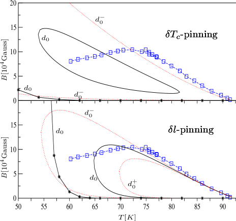
Figure 2: Unified BG-VG, VG-VL transition line $B_{m}(T)$ (31) as a function of the temperature. The curves in the upper figure are calculated for $\delta T_{c}$-pinning mechanism (10), the lower for $\delta_{l}$-pinning mechanism (11). The parameter $d_{0}$ of the solid curves are chosen such that we get a good fitting to the experimentally determined VG-VL line by Bouquet et al. Bouquet1 (dashed curve with square points) for both pinning mechanisms. The dotted curves are variations from these best fitting curves given by disorder parameters $d_{0}^{\pm}=(1\pm 1/2)\,d_{0}$ where $d_{0}$ are the disorder parameters of the solid curves of both mechanisms given by $2\pi d_{0}\,\xi^{2}_{ab}/{\xi^{\prime}}^{2}=8.5\cdot 10^{-8}$ ($\delta T_{c}$- pinning) and $2\pi d_{0}\,\xi^{2}_{ab}/{\xi^{\prime}}^{2}=1.01\cdot 10^{-6}$ ($\delta l$- pinning). The solid curves with the stars are calculated by solving (27) with elastic moduli in the range $b\lesssim 0.2$ with $d_{0}$ given above.

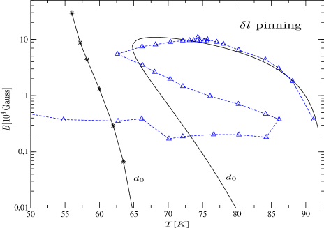
Figure 3: Logarithmic plot of the BG-VG, BG-VL first-order line $B_{m}(T)$ (31). The experimental points (triangles) correspond to the experiment of Pal et al. Pal1 showing a reentrant BG-VG line. The theoretical determined solid curves are derived from (31). The pure solid curve ($b\gtrsim 0.5$) and the solid curve with the stars ($b\lesssim 0.2$) correspond to the lower curves in Fig. 2 ($\delta l$-pinning). The theoretical curves are calculated with the disorder parameter $2\pi d_{0}\,\xi^{2}_{ab}/{\xi^{\prime}}^{2}=1.01\cdot 10^{-6}$ of Fig. 2.

Brandt Brandt1 determined the elastic constants for two different regimes $b\lesssim 0.2$ and $b\gtrsim 0.5$ where $b=B/H_{c2}(T)$. We shall see below that for YBCO we have to determine (27) in both regimes to find the entire relevant part of the BG-VG and BG-VL line. The most important part, however, lies in the regime $b\gtrsim 0.5$ which will now be treated explicitly. In this regime the elastic moduli $c_{44}$ and $c_{66}$ are given by Brandt1

$$c_{66}\! \!=\! \!0.71\,(1-b)\frac{B\phi_{0}}{64\pi^{2}\tilde{\lambda}_{ab}^{2}}\,,$$ (28)

$$c_{44}\! \!=\! \!\frac{B^{2}}{4\pi(1\!+\!\tilde{\lambda}_{c}^{2}k^{2}\!+\!\tilde{\lambda}_{ab}^{2}k_{3}^{2})}+\frac{B\phi_{0}}{16\pi^{2}\tilde{\lambda}_{c}^{2}}.$$ (29)

$\tilde{\lambda}=\lambda/(1-b)^{1/2}$ is the screened penetration depth calculated from the penetration depth $\lambda$. In $xy$-direction, we denote it by $\lambda_{ab}$, and in $z$-direction by $\lambda_{c}$. For YBCO we have Kamal1 $\lambda(T)=\lambda(0)[1-(T/T_{c})]^{-1/3}$, $\xi_{ab}(T)=\xi_{ab}(0)[1-(T/T_{c})]^{-1/2}$.

For later use, we define the Lindemann parameter Dietel2

$$c_{L}^{2}\! = \!\frac{a_{3}^{2}}{a^{2}v}\frac{k_{B}T}{V_{\rm BZ}}\int_{\rm BZ}\!\!d^{2}kdk_{3}\frac{1}{c_{44}}\sum_{i=1,6}\!\frac{1}{\frac{c_{ii}a_{3}^{2}}{c_{44}}K^{*}_{j}K_{j}+a_{3}^{2}K^{*}_{3}K_{3}}$$ (30)

$$\approx \frac{k_{B}T_{m}}{4\left[c_{44}(\frac{K_{\rm BZ}}{\sqrt{2}},0)\,c_{66}(\frac{K_{\rm BZ}}{\sqrt{2}},0)\right]^{1/2}a^{3}}\,.\$$

given by $c_{L}^{2}=\langle u^{2}\rangle_{T\to 0}/a^{2}$ where the average is taken with respect to the low-temperature Hamiltonian (14) representing the elastic energy of the vortex lattice. $K_{\rm BZ}$ is the boundary of the circular Brillouin zone $K_{\rm BZ}^{2}=4\pi B/\phi_{0}$. For YBCO, we obtain Dietel2 $c_{L}\approx 0.18$ on the melting line without disorder in accordance with typical Lindemann numbers for crystals GFCM2 . We note that this number does not depend on the magnetic field which specifies the point on the melting line. In the following we denote $c_{44}(K_{\rm BZ}/\sqrt{2},0)$ and $c_{66}(K_{\rm BZ}/\sqrt{2},0)$ in final expressions as for example in (30) by the abbreviations $c_{44}$ and $c_{66}$.

From (27) we can easily calculate the BG-VG, VG-VL line. By taking into account $c_{L}^{2}a^{2}\ll\xi^{\prime 2}$ which results in ${\cal D}(2\langle u^{2}\rangle)\approx{\cal D}(0)$ for YBCO we obtain for the unified BG-VG, VG-VL line

$$B_{m}\approx\frac{\phi_{0}^{5}\,(1-b)^{3}}{(k_{B}T)^{2}\lambda^{2}_{ab}\lambda^{2}_{c}}\frac{3.9\cdot 10^{-5}}{\pi^{4}}\;e^{-{\cal D}_{0}(0)}$$ (31)

Here we used $a=\sqrt{\phi_{0}}/\sqrt{B}$ and the typical defect length $a_{3}\approx 4a\sqrt{2}\,\lambda_{ab}/\lambda_{c}\sqrt{\pi}(1-b)^{1/2}$ Dietel2 , which results in the disorder function

$${\cal D}_{0}(0)\approx\left(d(T)\frac{\xi_{ab}^{2}}{\xi^{\prime 2}_{0}}\right)\frac{3.2\,(1-b)^{3/2}}{(k_{B}T)^{2}}\frac{\phi_{0}^{4}\,\xi_{ab}}{\lambda_{ab}^{3}\lambda_{c}}\frac{\phi_{0}^{1/2}}{B^{1/2}}\,.$$ (32)

Note that (31) is valid irrespective of the disorder correlation function.

Parameter values for optimally doped YBCO were given by Ref. Kamal1, as $\lambda_{ab}(0)\approx 1186$Å, $\xi_{ab}(0)\approx 15$Å, $T_{c}=92.7K$. The CuO₂ double layer spacing is $a_{s}=12$Å, and the anisotropy parameter $\gamma\equiv\lambda_{c}/\lambda_{ab}$ is approximately equal to $5$. From (32) we obtain a unified BG-VG, BG-VL line which scales like $B_{m}\sim e^{-A_{Y}/\sqrt{B_{m}}}$. Here $A_{Y}$ is some constant independent of $B_{m}$. This results in a BG-VG, BG-VL line showing a reentrant behavior. In Fig. 2 we show $B_{m}$ with $\delta T_{c}$-pinning on the upper figure and $\delta l$-pinning on the lower figure for various values $d_{0}$. $d_{0}$ of the straight line curves is chosen such that we have approximately the best experimental curve fitting to the BG-VG, BG-VL curve of Bouquet et al. Bouquet1 shown by the dashed line with square points. We obtain in fact a reentrant behavior of the BG-VG, BG-VL line. This is in accordance with the quadratic in disorder calculation for YBCO within the Ginzburg-Landau approach by Li et al. Li1 . A reentrant behavior of the BG-VG line was also seen in the experiments of Pal et al. Pal1 and Stamopoulos et al. Stamopoulos1 . We must clarify that these experiments are in contradiction to the majority of experiments which do not see any reentrant behavior of the BG-VG line (see for example Bouquet1 ; Deligiannis1 ; Radzyner1 ; Nishizaki1 ; Griessen1 ). The discrepancy in the shape of the BG-VG transition line lies presumably in different physical setting of these experiments to the standard ones showing no reentrant behavior. The experiment of Pal et al. uses a crystal with a low density of twins which could lead to deviations in the shape of the BG-VG line due to Miu1 . The experiments of Stamopoulos et al. measures the ac permeabilities which drives the crystal out of thermodynamical equilibrium.

The solid lines with the stars at the left hand side of Fig. 2 are calculated by solving (27) restricted to the transverse fluctuations with the elastic moduli in the range $b\lesssim 0.2$ given in Brandt1 ; Dietel2 . To calculate the transition curves with the elastic moduli $b\lesssim 0.2$ as well is rather important because the solid curves in Fig. 2 calculated with moduli $b\gtrsim 0.5$ reaches immediately the range $b\lesssim 0.2$. Note that the solid curves and the solid curves with stars are calculated by using the same disorder constant $d_{0}$ of values $2\pi d_{0}\,\xi_{ab}^{2}/{\xi^{\prime}}^{2}=8.5\cdot 10^{-8}$ ($\delta T_{c}$- pinning) and $2\pi d_{0}\,\xi_{ab}^{2}/{\xi^{\prime}}^{2}=1.01\cdot 10^{-6}$ ($\delta l$-pinning).

We obtain from Fig. 2 that the curves of the $\delta l$-pinning mechanism fits much better to the experimentally given BG-VG, BG-VL line than the $\delta T_{c}$-pinning curves. This is in accordance to the observation in Ref. Griessen1, . Whatever the correct experimental BG-VG, BG-VL line shows a reentrant behavior or not, it is not satisfactory within our approach which is restricted to second order in the impurity potential, that the solid curves with the stars ($b\lesssim 0.2$) goes to zero at $T\approx T_{c}$. That this is true can be best seen in a logarithmic plot of the BG-VG, BG-VL transition line $B_{m}$ (31) which is shown in Fig. 3. The straight line and the straight line with the stars correspond to the curves of the $\delta l$-pinning mechanism shown in the lower part in Fig. 2. The dashed curve with the triangle points is the BG-VG, BG-VL line measured by Pal et al. in Ref. Pal1, mentioned above. This curve shows a reentrant behavior. Both curves are in disagreement at small magnetic fields. Thus, we should go beyond second order in the disorder strength to get better accordance with the experiments. This will be done in the following sections.

V Replica variational method of Mézard and Parisi

In order to go beyond second-order perturbation theory in the impurity potential, we use the well known replica trick Edwards1 $\ln Z=\lim_{n\to 0}(1/n)(\overline{Z^{n}}-1)$ where the overline means disorder averaging and

$$\overline{Z^{n}}=\left[\prod_{\alpha}\int{\cal D}[u^{\alpha}_{i},\sigma^{\alpha}_{im},n^{\alpha}_{i}]\right]$$

$$~{}~{}~{}~{}~{}~{}~{}~{}~{}~{}~{}~{}~{}~{}~{}~{}~{}~{}\times\overline{e^{-\Sigma_{\alpha}\left(H_{0}[u^{\alpha}_{i},\sigma^{\alpha}_{im},n^{\alpha}_{i}]+H_{\rm dis}[u^{\alpha}_{i}]\right)/k_{B}T}}$$

$$=\left[\prod_{\alpha}\int{\cal D}[u^{\alpha}_{i},\sigma^{\alpha}_{im},n^{\alpha}_{i}]\right]e^{-\Sigma_{\alpha}H_{0}[u^{\alpha}_{i},\sigma^{\alpha}_{im},n^{\alpha}_{i}]/k_{B}T}$$

$$~{}~{}~{}~{}~{}~{}~{}~{}~{}~{}~{}~{}~{}~{}~{}~{}~{}~{}\times e^{-\Sigma_{\alpha,\beta}H^{\prime}_{\rm dis}[u^{\alpha}_{i},u^{\beta}_{i}]/k_{B}T},$$ (33)

with

$$H^{\prime}_{\rm dis}[u^{\alpha}_{i},u^{\beta}_{i}]=\frac{-1}{2k_{B}T}\sum_{{\bf x},{\bf x}^{\prime}}\delta_{x_{3},x_{3}^{\prime}}\Delta(x_{i}+u_{i}^{\alpha}({\bf x})-x^{\prime}_{i}-u_{i}^{\beta}({\bf x}^{\prime}))\,.$$ (34)

Here, the extra $k_{B}T$ term in the denominator in (34) comes from the disorder average.

The average $\overline{Z^{n}}$ cannot be calculated without further approximations. In the following we use the low- and high-temperature approximations of Section III for the result after the integration over the stress fields $\sigma_{ij}^{\alpha}$ and defect fields $n_{i}^{\alpha}$ in $\overline{Z^{n}}$ (33). Thus, we have to calculate partition functions of the following form

$$\overline{Z^{n}} = \left[\prod_{\alpha}{\cal N}\prod_{{\bf x},i}\left[\int_{-\infty}^{\infty}\frac{u^{\alpha}_{i}({\bf x})}{a}\right]\right]$$ (35)

$$\times e^{-H/k_{B}T},$$

with the total Hamiltonian

$$H=\sum_{\alpha}H_{0}[u_{i}^{\alpha}]+\sum_{\alpha,\beta}H^{\prime}_{\rm dis}[u_{i}^{\alpha},u_{i}^{\beta}],$$ (36)

where $H_{0}$ is given by (14) in the solid phase and by (15) in the fluid phase. Both are complicated expressions which will need further approximations. The complications comes from the large replica mixing interaction part $H^{\prime}_{\rm dis}$ in (33). In the following, we shall use a variational replica method which was first given by Mézard and Parisi Mezard1 . With the help of this method also used before for random spin models Dotsenko1 they were able to calculate the glass transitions of isotropic random manifold systems. These systems are described by the Hamiltonian

$$H_{\rm RM}=\int d^{d-N^{\prime}}\!\!x\,[-{\bf u}({\bf x})({\mbox{\boldmath$\nabla$}}\cdot{\mbox{\boldmath$\nabla$}}){\bf u}({\bf x})+V({\bf u})]\,.$$ (37)

Here ${\bf u}$ is an $N^{\prime}$-dimensional vector describing an $N^{\prime}$-dimensional manifold embedded in a $d$-dimensional space. $V$ is an impurity potential with a certain correlation function. When comparing the solid Hamiltonian (14) with the random manifold Hamiltonian (37) and further by setting the correlation length $\xi^{\prime}=0$ in (21) we obtain that the transversal part of (14) looks similar to a random manifold with $d-N^{\prime}=3$ in $d=5$ dimensions Mezard1 with a delta-like impurity correlation potential. In the fluid phase described by the high-temperature Hamiltonian (15) we obtain for the transversal part a random manifold with $d-N^{\prime}=1$ and $d=3$ well known as a string embedded in three dimensions. The difference to the random manifold system comes then mainly from the discretization in the third direction by the dislocation length $a_{3}$ relevant in the fluid phase as will be shown below. It is well known that there exist for $N^{\prime}>2$ in a $d=N^{\prime}+1$ random manifold system corresponding to a string in $d$ dimensions a roughening transition separating a low-temperature disorder dominated phase from a high-temperature thermal phase Halpin1 . For $N^{\prime}<2$ this phase transition is not existent and the system is dominated mainly by disorder fluctuations. It is now believed by computer simulations that at the critical dimension $N^{\prime}=2$ corresponding to a string in three dimensions with a $\delta$-correlated impurity potential the roughening transition of the string system is described by a crossover Halpin1 . Below we show that this roughening transition corresponds to the glass transition of the vortex lattice. That the vortex lattice at $d=3$ is in fact at the lower critical dimension for a glass transition was mentioned before for an XY-model of the gauge class type Reger1 . This XY-model as similar ones with other disorder potentials mentioned in the introduction are toy model for a disordered vortex lattice in superconductors.

The Mézard-Parisi theory consists in replacing the non-quadratic part of the Hamiltonian as quadratic with a possible mixing of replica fields. By using the Bogoliubov variational principle we can find the best matrix of this quadratic form so that the free energy of the variational Hamiltonian is as close as possible to the actual free energy of the system. This means that we have to search the minimum of the variational free energy

$$F_{\rm var}=F_{\rm trial}+\langle H-H_{\rm trial}\rangle_{\rm trial}$$ (38)

with the harmonic trial Hamiltonian

$$H_{\rm trial}=\frac{v}{2}\sum_{{\bf x},{\bf x}^{\prime}}\sum_{\alpha,\beta}{\bf u}^{\alpha}({\bf x}){\bf G}^{-1}_{\alpha\beta}({\bf x}-{\bf x}^{\prime}){\bf u}^{\beta}({\bf x}^{\prime})\,.$$ (39)

Here $\langle\cdot\rangle_{\rm trial}$ stands for the averaging with respect of the Gibb’s measure of the trial Hamiltonian $H_{\rm trial}$, and $F_{\rm trial}$ denotes the associated free energy. In Section  IX, we shall use the intersection criterion with $F_{\rm var}$ for the solid and fluid phase to determine the BG-VG, BG-VL transition line. By using (39), we obtain the free energy associated with (35):

$$F_{\rm var}=-k_{B}T\frac{N}{2V_{\rm BZ}}\int_{\rm BZ}d^{2}kdk_{3}\;\bigg{(}\ln\left[{\rm det}\,\left(\frac{2\pi k_{B}T}{va^{2}}{\bf G}\right)\right]$$

$$+{\rm Tr}\left\{\left[{\bf G}^{-1}({\bf k})-{\bf G}_{0}^{-1}({\bf k})\,{\rm I}\right]{\bf G}({\bf k})\right\}\bigg{)}$$

$$-k_{B}T\ln({\cal N})+\left\langle\sum_{\alpha,\beta}H^{\prime}_{\rm dis}[u_{i}^{\alpha},u_{i}^{\beta}]\right\rangle_{\rm trial}\,.$$ (40)

where we use bold symbols for vectors and matrices in the vortex displacement plane. The symbol ${\rm I}$ denotes the unit matrix in replica space. The trace ${\rm Tr}[\,\dots\,]$ runs over the replica indices and vortex displacement indices. In principle we can obtain a general expression for the disorder term given by the last term in (40). Because one should use different approximations for the solid phase and the liquid phase, we shall give directly approximations for this term in both phases at the beginning of the following sections.

It will be clear soon for the solid as well as the fluid phase that ${\bf G}_{\alpha\beta}$ can be chosen to have the form

$${\bf G}^{-1}_{\alpha\beta}={\bf G}_{0}^{-1}\delta_{\alpha\beta}+\sigma_{\alpha\beta}\,{\bf I}$$ (41)

where ${\bf I}$ is the two-dimensional unit matrix in the vortex displacement plane. To find a local minimum of (40) in the space of all symmetric self-energy matrices $\sigma_{\alpha\beta}$ was simplified considerably by Parisi in the case of spin glasses. There he restricted the search of the minimum for (38) to the case of some sort of closed algebra known as the algebra of Parisi matrices Dotsenko1 ; Mezard2 . In Appendix B we prove some stability theorems for stationary points of $F_{\rm var}$ (40). These are summarized at the end of Appendix B2. The restriction of the minimum search to self-energy matrices in the Parisi-algebra is justified among others by the fact that a local minimum within the Parisi-algebra is automatically a local minimum in the whole self-energy space without the restriction to the Parisi-algebra. This is shown in Appendix B.

In general the minimum self-energy matrix $\sigma_{\alpha\beta}$ is not symmetric under the interchange of replica indices which means that the local minimum $\sigma_{\alpha\beta}$ of $F_{\rm var}$ (40) is not unique. This is typical for glasses where the minimum of the free energy is degenerate Dotsenko1 . This degeneracy corresponds to the degeneracy of the stable states in glasses with high energy barriers between them. These are responsible for the irreversibility phenomena beyond the glass transition lines in high-temperature superconductors mentioned in the introduction.

VI Fluid phase

In this section, we derive the variational free energy $F_{\rm var}$ in the liquid phase. We obtain

$$\left\langle\sum_{\alpha,\beta}H^{\prime}_{\rm dis}[u_{i}^{\alpha},u_{i}^{\beta}]\right\rangle_{\rm trial}\approx-\frac{N}{2k_{B}T}\sum_{\alpha,\beta}\frac{1}{(2\pi)^{2}}$$

$$\times\int d^{2}q\;\hat{\Delta}(q)e^{-\frac{1}{2}{\bf q}\!\cdot\!\bigg{[}\!{\bf G}_{\alpha\alpha}(0)+{\bf G}_{\beta\beta}(0)-{\bf G}_{\alpha\beta}(0)-{\bf G}_{\beta\alpha}(0)\!\bigg{]}{\bf q}}$$

$$\approx-k_{B}T\,\frac{N}{2}\sum_{\alpha,\beta}{\cal D}\left(2B_{\alpha\beta}\right)$$ (42)

with

$$B_{\alpha\beta}=\frac{k_{B}T}{2v}{\rm tr}\left[{\bf G}_{\alpha\alpha}(0)+{\bf G}_{\beta\beta}(0)-{\bf G}_{\alpha\beta}(0)-{\bf G}_{\beta\alpha}(0)\right]\,.$$ (43)

where $\tilde{\Delta}({\bf q})$ is the two-dimensional Fourier transform of $\Delta({\bf x})$. The trace ${\rm tr}[\,\dots\,]$ runs over the vortex displacement indices. In (42) we restricted us in the double sum over ${\bf x}$, ${\bf x}^{\prime}$ on the diagonal summands ${\bf x}={\bf x}^{\prime}$. The reason for the validity of this restriction comes from the observation that due to (15) the non-diagonal summands are given by

$$\left[\left\langle\sum_{\alpha,\beta}H^{\prime}_{\rm dis}[u_{i}^{\alpha},u_{i}^{\beta}]\right\rangle_{\rm trial}\right]_{{\bf x}\not={\bf x}^{\prime}}\!\!\!\!=-\frac{1}{2k_{B}T}\sum_{{\bf x}\not={\bf x}^{\prime}}$$

$$\times\delta_{x_{3},x_{3}^{\prime}}\sum_{\alpha,\beta}\frac{1}{(2\pi)^{2}}\int d^{2}q\;\hat{\Delta}({\bf q})e^{iq_{i}(x_{i}-x_{i}^{\prime})}$$ (44)

$$\times e^{-\frac{1}{2}{\bf q}\cdot\left[{\bf G}^{T}_{\alpha\alpha}(0)+{\bf G}^{T}_{\beta\beta}(0)-{\bf G}^{T}_{\alpha\beta}({\bf x}-{\bf x}^{\prime})-{\bf G}^{T}_{\beta\alpha}({\bf x}-{\bf x}^{\prime})\right]{\bf q}}$$

$$\times e^{-\frac{1}{2}{\bf q}\cdot\left[{\bf G}^{L}_{\alpha\alpha}(0)+{\bf G}^{L}_{\beta\beta}(0)-{\bf G}^{L}_{\alpha\beta}({\bf x}-{\bf x}^{\prime})-{\bf G}^{L}_{\beta\alpha}({\bf x}-{\bf x}^{\prime})\right]{\bf q}}$$

where ${\bf G}^{L}={\bf P}_{L}{\bf G}{\bf P}_{L}$ and ${\bf G}^{T}={\bf P}_{T}{\bf G}{\bf P}_{T}$ are the longitudinal and transversal components of the Green function. By using (15) the second exponent in (44) corresponding to the transversal part of the vortex fluctuations can be tranformed to

$$-\frac{1}{2}\bigg{\{}({\bf q}^{T})^{2}(0)\,[G^{T}_{\alpha\alpha}(0)+G^{T}_{\beta\beta}(0)]$$

$$-({\bf q}^{T})^{2}({\bf x}-{\bf x}^{\prime})\;[G^{T}_{\alpha\beta}(0)+G^{T}_{\beta\alpha}(0)]\bigg{\}}$$ (45)

where $G^{L,T}_{\alpha\beta}({\bf x})={\rm Tr}[{\bf G}^{L,T}_{\alpha\beta}({\bf x})]$. Due to the large thermal effective one-dimensional transverse fluctuations we have either $G^{T}_{\alpha\beta}(0)\rightarrow\infty$ where $G^{T}_{\alpha\alpha}(0)-G^{T}_{\alpha\beta}(0)$ is finite and $\alpha$, $\beta$ is arbitrary or $G^{T}_{\alpha\alpha}(0)\rightarrow\infty$ and $G^{T}_{\alpha\beta}(0)$ is finite for $\alpha\not=\beta$ where in both cases the self-energy matrix is restricted to the Parisi algebra. This is shown in Ref. Mezard1, . From this we obtain the vanishing of (44).

First, we take the variation of the free energy (40) with respect to the diagonal Green function matrix elements $G_{\alpha\alpha}$. This results in

$$\sum_{\beta}\sigma_{\alpha\beta}=0$$ (46)

That the minimum of $F_{\rm var}$ should be found in the symmetric self-energy matrices with the constraint (46) is suggestive because (46) justifies that the Hamiltonian (39) has the global translational symmetry ${\bf u}^{\alpha}({\bf x})\rightarrow{\bf u}^{\alpha}({\bf x})+{\bf t}$ for any vector $t$, which has also the disorder Hamiltonian (34).

In the most general case within the Parisi-algebra, the form of the self-energy $\sigma_{\alpha\beta}$ with the constraint (46) can be described by a continuous function $\sigma(s)$ with $0<s<1$ Mezard1 . In that case the trial free energy takes the form

$$\Delta f_{\rm var}\equiv\frac{1}{N}\lim_{n\to 0}\frac{1}{n}\left[F_{\rm var}(B[\Delta])-F_{\rm var}(0)\right]$$ (47)

$$=\frac{k_{B}T}{2}\int_{0}^{1}ds\;\bigg{[}\frac{1}{s^{2}}\int_{0}^{\Delta(s)}\!\!\!\!\!d\Delta\Delta\frac{d}{d\Delta}g(\Delta)+{\cal D}_{0}\left(2B[\Delta(s)]\right)\bigg{]}$$

$$f_{\rm var}(0)=\frac{1}{N}{\rm lim}_{n\to 0}\frac{1}{n}F_{\rm var}(0)=-k_{B}T\bigg{(}\frac{1}{N}\ln{\cal N}$$ (48)

$$+\frac{1}{2}\bigg{\{}\frac{1}{V_{\rm BZ}}\int_{\rm BZ}d^{2}kdk_{3}\;\ln\left[{\rm det}\,\left(\frac{2\pi k_{B}T}{va^{2}}{\bf G}_{0}\right)\right]+{\cal D}_{0}(0)\bigg{\}}\bigg{)}$$

where

$$g(\Delta)=\frac{1}{V_{\rm BZ}}\int_{\rm BZ}d^{2}kdk_{3}{\rm Tr}\left[\left({\bf G}_{0}^{-1}+\Delta{\bf I}\right)^{-1}\right]\,.$$ (49)

The gap function $\Delta(s)$ and the self-energy function $\sigma(s)$ corresponding to the self-energy matrix $\sigma_{\alpha\beta}$ in the non-continuous case is related by

$$\Delta(s)=\int_{0}^{s}ds^{\prime}s^{\prime}\frac{d\sigma(s^{\prime})}{ds^{\prime}}\,.$$ (50)

$B[\Delta(m)]$ corresponding to $B_{\alpha\beta}$ (43) in the continuous case is given by

$$B[\Delta(s)]=\frac{k_{B}T}{v}\frac{1}{s}g[\Delta(s)]-\frac{k_{B}T}{v}\int_{s}^{1}ds^{\prime}\frac{1}{s^{\prime 2}}g[\Delta(s^{\prime})]\,.$$ (51)

In order to find the local minimum of $f_{\rm var}$ we have to take the derivative of (47) with respect to $\Delta(m)$. This results in

$$\sigma(s)=-2\,\frac{k_{B}T}{v}\;{\cal D}^{\prime}_{0}\left(2B[\Delta(s)]\right)\,,$$ (52)

where $D^{\prime}(x)$ is the derivative $(d/dx)D(x)$. We point out that (52) shows that

$$\sigma(s)\geq 0\quad,\qquad\Delta(s)\geq 0\,.$$ (53)

In the following, we discuss solutions of this equation in the case that $\sigma(s)$ does not break the replica symmetry, is one-step replica symmetry-breaking or continuous replica symmetry-breaking.

VI.1 Symmetric solution

We now solve Eq. (52) for $\sigma(s)$ with an Ansatz which does not break any replica symmetry. The Ansatz for $\sigma(s)$ in this case is

$$\sigma(s)=\sigma_{0}\,.$$ (54)

By using the equations (50) and (52) we obtain

$$\sigma(s) = 0\,,$$ (55)

$$\Delta(s) = 0\,.$$ (56)

From this we obtain that $B[\Delta(m)]\rightarrow\infty$ for infinite area of the system. This results in

$$\Delta f_{\rm var}=0\,.$$ (57)

VI.2 One-Step replica symmetry-breaking

The simplest possible extension of the replica symmetric case above consists of a one-step replica symmetric solution given by

$$\sigma(s)=\left\{\begin{array}[]{ccc}\sigma_{0}&\mbox{for}&0<s<m_{1}\,,\\ \sigma_{1}&\mbox{for}&m_{1}<s<1\,.\end{array}\right.$$ (58)

By using this Ansatz in (47) we obtain

$$\Delta f_{\rm var}=-\frac{k_{B}T}{4}\left(1-\frac{1}{m_{1}}\right)$$

$$\times\left[\left(\frac{\tilde{\Delta}_{1}}{1+\tilde{\Delta}_{1}/4}\right)^{1/2}\!\!\!\!\!\!\!\!\!\!-4\,{\rm arcsinh}\left(\frac{\tilde{\Delta}^{1/2}_{1}}{2}\right)\right]$$

$$+\frac{k_{B}T}{2}(1-m_{1}){\cal D}\left(2\frac{k_{B}T}{v}g(\Delta_{1})\right)$$ (59)

where we used $\sigma_{0}=0$ which can be derived from (52) and (50) similar to the replica symmetric case. Furthermore, we used the abbreviation $\Delta_{1}=m_{1}(\sigma_{1}-\sigma_{0})=m_{1}\sigma_{1}$ and $\tilde{\Delta}_{i}\equiv\Delta_{i}a_{3}^{2}/c_{44}$. We restricted us in the calculation of $\Delta f_{\rm var}$ to the transversal components of ${\bf G_{0}}$ which effectively means that we set $G_{0}^{L}=0$ in the calculation $g(\Delta)$ in (49). The longitudinal term in $g(\Delta)$ is a factor $a^{2}c_{44}/a^{2}_{3}c_{11}=(a^{2}c_{44}/a^{2}_{3}c_{66})(c_{66}/c_{11})\approx(\pi/4)(c_{66}/c_{11})$ smaller which is justified by $c_{66}\ll c_{11}$ Brandt1 irrespective of the value of $\tilde{\Delta}_{1}$. For the derivation of $\Delta f_{\rm var}$ we used for $g(\Delta)$ in (49)

$$g(\Delta) \approx \frac{a_{3}^{2}}{c_{44}}\frac{1}{V_{\rm BZ}}\int_{\rm BZ}d^{2}kdk_{3}\frac{1}{[2-2\cos(k_{3}a_{3})]+\tilde{\Delta}}$$ (60)

$$= \frac{1}{2}\frac{1}{\tilde{\Delta}^{1/2}(1+\tilde{\Delta}/4)^{1/2}}\frac{a^{2}_{3}}{c_{44}}\,.$$

We now determine the stationary point of $\Delta f_{\rm var}$ (59). By setting the derivative of $\Delta f_{\rm var}$ with respect to $\Delta_{1}$ and $m_{1}$ equal to zero we obtain two equations for the stationary values of $\Delta_{1}$ and $m_{1}$. These are given by

$$\frac{1}{8}\left(1-\frac{1}{m_{1}}\right)\tilde{\Delta}_{1}^{-1/2}=\frac{1}{4}\left(1-m_{1}\right)\frac{k_{B}T}{\tilde{\Delta}_{1}^{3/2}}\frac{a_{3}}{c_{44}a^{2}}$$

$$\times{\cal D}^{\prime}\left(2\frac{k_{B}T}{v}g(\Delta_{1})\right)\,,$$ (61)

$$\frac{1}{4}\frac{1}{m_{1}^{2}}\left[4{\rm arcsinh}\left(\frac{\tilde{\Delta}^{1/2}_{1}}{2}\right)-\left(\frac{\tilde{\Delta}_{1}}{1+\tilde{\Delta}_{1}/4}\right)^{1/2}\right]$$

$$=\frac{1}{2}\;{\cal D}\left(2\frac{k_{B}T}{v}g(\Delta_{1})\right)\,.$$ (62)

In the following solution of (61) and (62) we use that $\tilde{\Delta}_{1}\ll 1$ in the interesting range near the glass transition line which we expect at $\tilde{\Delta}_{1}=0$. This will be shown below. These two equations can be solved exactly in this limit resulting in

$$m_{1}^{3} = ({\cal D}(0)A)^{-1}\,,$$ (63)

$$\tilde{\Delta}_{1}^{1/2} = 2A^{-1}\left(\frac{1}{m_{1}}-1\right)$$ (64)

where constant $A$ similar to the Lindemann constant written for general disorder correlation functions (see the definitions (19)-(23))

$$A_{0,\infty}=\frac{4}{k_{B}T}\frac{c_{44}a^{2}\;{\xi^{\prime}}^{2}_{0,\infty}}{a_{3}}\,.$$ (65)

with $A\equiv A_{0}=A_{\infty}$ for the Gaussian correlation function (12). Here, we mention that $A\approx b/2\pi c_{L}^{2}\gg 1$ near the melting line without disorder $V=0$ Dietel2 . This is the magnetic-temperature regime, we are interested in. By the help of (59), (63) and (64) we can calculate the free energy $\Delta f_{\rm var}$ getting

$$\Delta f_{\rm var}=\frac{k_{B}T}{2}{\cal D}_{\infty}(0)\left[1-({\cal D}_{\infty}(0)A_{\infty})^{-1/3}\right]^{3}$$ (66)

for ${\cal D}_{\infty}(0)A_{\infty}\geq 1$ in the regime $(({\cal D}(0)A)^{1/3}-1)/A\ll 1$ for the Gaussian correlation function (12). As suggested by the indices, expression (66) is more general valid irrespective of the disorder correlation potential in the restricted regime $(({\cal D}_{\infty}(0)A)_{\infty}^{1/3}-1)\ll 1$ (see the discussion above Eq.  (92)). Next, we must calculate also the replica symmetry-breaking solutions of the free energy (47) having more than one discrete step. To solve the minimum problem in this case is rather difficult. Therefore, we restrict us first to the determination of the continuous symmetry-breaking solutions.

VI.3 Continuous symmetry breaking

Finally, we look for solutions $\sigma(s)$ of (52) which are continuous. In this case, we can solve the stationary equation by a partial integration of $B[\Delta(s)]$ in (51) resulting in Giamarchi1

$$B[\Delta(s)]=B[\Delta(s_{c})]-\frac{k_{B}T}{v}\int_{s}^{s_{c}}ds^{\prime}\sigma^{\prime}(s^{\prime})g^{\prime}(\Delta[s^{\prime}])\,.$$ (67)

Here we assumed that $\sigma(s)={\rm constant}$ for $s\geq s_{c}$. By taking two derivatives of (52) we obtain that $\sigma(s)$ fulfills the following equation

$$\sigma^{\prime}(s)=-2\sigma^{\prime}(s)\sigma(s)^{3/2}\frac{(k_{B}T)^{1/2}}{\xi^{\prime}{\cal D}^{1/2}(0)}\frac{1}{v^{1/2}}g^{\prime}(\Delta[s])\,.$$ (68)

Similar as in the case of the one-step symmetry-breaking solution we can neglect the longitudinal component in $g(\Delta)$ (49) being a factor $c_{66}/c_{11}\ll 1$ smaller than the transverse term in $g(\Delta)$ (see the discussion below (59)). We point out that this is true irrespective of the value of $\Delta$. Using (60) we obtain two solutions of (68) by taking once more the derivative with respect to $s$. This results in the following solutions of (68)

$$1.\quad\sigma^{\prime}(s)=0\,,$$ (69)

$$2.\quad\left(\frac{a^{2}_{3}}{c_{44}}\right)\sigma(s)\,s=\frac{\tilde{\Delta}(s)\left[1+\frac{1}{4}\tilde{\Delta}(s)\right]\left[1+\frac{5}{4}\tilde{\Delta}(s)\right]}{1+\frac{2}{3}\tilde{\Delta}(s)+\frac{1}{6}\tilde{\Delta}^{2}(s)}\,.$$ (70)

By inserting (68) into (70) we obtain for the second type of solutions

$$s\,({\cal D}(0)A)^{1/3}=\frac{\left[1+\frac{5}{4}\tilde{\Delta}(s)\right]^{5/3}}{1+\frac{2}{3}\tilde{\Delta}(s)+\frac{1}{6}\tilde{\Delta}^{2}(s)}\,.$$ (71)

Finally, we determine the constant $s_{c}$ defined in (67) where $\sigma(s)={\rm constant}$ for $s_{c}<s<1$. By using (52) we obtain

$$\sigma(s_{c})=-2\frac{k_{B}T}{v}\,{\cal D}^{\prime}\left(2B[\Delta(s_{c})]\right)\,.$$ (72)

With the help of (70) we obtain

$${\cal D}(0)As_{c} = \frac{\left[1+\frac{5}{4}\tilde{\Delta}(s_{c})\right]}{1+\frac{2}{3}\tilde{\Delta}(s_{c})+\frac{1}{6}\tilde{\Delta}^{2}(s_{c})}$$

$$\times\left\{\frac{1}{2}A\;\tilde{\Delta}^{1/2}(s_{c})\left[1+\frac{1}{4}\tilde{\Delta}(s_{c})\right]^{1/2}+1\right\}^{2}$$

which leads with (71) to

$$({\cal D}(0)A)=\frac{\left\{\frac{1}{2}A\;\tilde{\Delta}^{1/2}(s_{c})\left[1+\frac{1}{4}\tilde{\Delta}(s_{c})\right]^{1/2}+1\right\}^{3}}{\left[1+\frac{5}{4}\tilde{\Delta}(s_{c})\right]}\,.$$ (74)

Under consideration of (53) we obtain that (74) can be solved only for ${\cal D}(0)A\geq 1$. Furthermore, by taking into account (71) in the case of $\tilde{\Delta}=0$ which is the same equation when taking only the most leading $\tilde{\Delta}$-term for $\tilde{\Delta}\rightarrow 0$ in (60), we obtain in this limit no solution of (71). As mentioned above, this corresponds to the marginality of a string in $d=3$ dimensions in an impurity background. Due to the non-quadratic polynomial behavior of the expressions above, it is not possible to get simple analytic solutions in the whole $\tilde{\Delta}$-range. Therefore, we shall solve (69), (71) and (VI.3) for small $\tilde{\Delta}\ll 1$. This corresponds to the restriction $(({\cal D}(0)A)^{1/3}-1)/A\ll 1$. We obtain in this range the following solutions:

$$\tilde{\Delta}(s)=\!\left\{\!\!\begin{array}[]{ccc}0&\mbox{for}&0\leq s\leq\frac{1}{({\cal D}(0)A)^{1/3}}\\ \frac{12}{17}\left[({\cal D}(0)A)^{1/3}s-1\right]&\mbox{for}&\frac{1}{({\cal D}(0)A)^{1/3}}\leq s\leq s_{c}\\ \frac{4}{A^{2}}\left[({\cal D}(0)A)^{1/3}-1\right]^{2}&\mbox{for}&s_{c}\leq s\leq 1.\end{array}\right.$$ (75)

with

$$s_{c}\approx\frac{1}{({\cal D}(0)A)^{1/3}}+\frac{17}{3}{\cal D}^{2}(0)\frac{(({\cal D}(0)A)^{1/3}-1)^{2}}{({\cal D}(0)A)^{7/3}}$$ (76)

Finally, we can calculate the free energy $\Delta f_{\rm var}$ for the replica symmetry-breaking solution (75) by using (47), (60) and (70) for $(({\cal D}(0)A)^{1/3}-1)/A\ll 1$. We obtain

$$\Delta f_{\rm var}=\frac{k_{B}T}{2}{\cal D}_{\infty}(0)\left[1-({\cal D}_{\infty}(0)A_{\infty})^{-1/3}\right]^{3}$$ (77)

identical with the free energy of the one-step replica symmetry breaking solution (66). (77) is valid for $(({\cal D}(0)A)^{1/3}-1)/A\ll 1$ in the case of a Gaussian disorder potential. But one can generalize the calculation above to obtain the validity of (77) in the smaller regime $(({\cal D}_{\infty}(0)A_{\infty})^{1/3}-1)\ll 1$ irrespective of the disorder correlation function (see the discussion above Eq. (92)). Summarizing, we obtain a saddle point of $\Delta f_{\rm var}$ which is symmetric in replica space for ${\cal D}_{\infty}(0)A_{\infty}\leq 1$. In the case of ${\cal D}_{\infty}(0)A_{\infty}\geq 1$ we obtain a replica-symmetric solution, a one-step replica symmetry-breaking solution and also a continuous replica symmetry-breaking solution appears. To get more insight into the true minimum, we have to consider the stability of the various saddle point solutions in this case.

VII Stability of solutions

In this section we determine whether the various solutions for the fluid phase discussed in the last section are stable in a sense specified below and whether we have to take into account also higher-step replica symmetry-breaking solutions to get a stable saddle point. A typical example of an exactly solvable system with finite-step replica symmetry-breaking saddle point solutions which are not stable is a string in two dimensions with a $\delta$- impurity correlation function resulting in an unphysical negative variance of the free energy with respect to disorder averaging Saakian1 . This negative variance is vanished in the case of the infinite or continuous replica symmetry-breaking solution. Mézard and Parisi Mezard1 show two different ways to obtain a theory which includes replica symmetry breaking such as (47)-(52) for random manifolds. The first approach consists of a large $N^{\prime}$ expansion of the partition function where $N^{\prime}$ is the number of components of the fields. There is only a slight difference between the large $N^{\prime}$ approach and the variational approach used above. In the saddle point equation of the large $N^{\prime}$-approach we have to substitute ${\cal D}(x)$ in (47)-(52) by $\Delta(\sqrt{x})/(k_{B}T)^{2}$ for the application of this approach to the fluid phase of the vortex lattice. This is discussed in Appendix B. The large $N^{\prime}$ expansion consists effectively in a saddle point approximation in suitable chosen auxiliary fields Mezard1 . The stability of solutions of these equations consists in going one step further to the quadratic expansion of the action in these auxiliary fields with the requirement that the partition function calculated from this saddle point approximation is not divergent when integrating out the auxiliary fields. It was shown by Carlucci et al. Carlucci1 that continuous replica symmetry-breaking solutions calculated in the last subsection are generally stable in this sense. This is reviewed by us in Appendix B1. Due to the smallness of $N^{\prime}=2$ in the vortex lattice system we do not think that the large $N^{\prime}$-expansion is appropriate in our case.

We derived (47)-(52) by another way also stated first by Mézard and Parisi Mezard1 via the variational approach in (38). It is clear that in this case we should require for the eigenvalues of the matrix built of the second derivatives of $\Delta F_{\rm var}$ with respect to the self-energies $\sigma_{\alpha\beta}$ that these are all positive in the stationary point. Here we take further into account the symmetry of $\sigma_{\alpha\beta}$ and (46) in the variation of the free energy. The concrete derivation was carried out by Šášik in Ref. Sasik1, . Starting from his expression for the Hessian we carry out in Appendix B2 a similar stability analysis as was done in the large $N^{\prime}$ case by Carlucci et al. in Ref. Carlucci1, summarized in Appendix B1. We also find in the variational approach that the continuous symmetry-breaking solutions are generally stable which means that all eigenvalues of the Hessian are larger than or equal to zero. Furthermore, we show in Appendix B2 that the full Hessian has positive or zero eigenvalues if and only if the replicon sector consists of positive or zero eigenvalues. Thus it is enough to consider only the replicon sector for stability. The lowest eigenvalues in the replicon sector Carlucci1 are given in (127) where $k=l=r+1$. Here $\tilde{f}$ is replaced by the disorder function ${\cal D}$ in our case and $L^{\prime}_{kl}$ is given in (117). $G_{0}$ is the transversal Green with zero self-energy and $G_{\alpha}$, $\Delta_{\alpha}$ are the value of the transversal full Green function and gap function in the Paris block $1\leq\alpha\leq R+1$ in a Parisi hierarchy of level $R$.

We now come to a discussion of the stability of the saddle point solutions in the fluid high-temperature phase in the symmetric form given in Section VIA and the one-step replica symmetric form given in Section VIB.

First, we consider the saddle point solution given in Section VIA for the replica symmetric form. The most relevant replicon eigenvalue $\tilde{\lambda}(0;1,1)$ is given by (127)

$$\tilde{\lambda}(0;1,1)\propto 1+4\frac{(k_{B}T)^{2}}{v^{2}}D^{\prime\prime}\left(2\frac{k_{B}T}{v}g(0)\right)g^{\prime}(0)$$ (78)

Here the proportionality factor is positive. The stability criterion $\tilde{\lambda}(0;1,1)\geq 0$ leads to

$${\cal D}(0)A\leq 1\,.$$ (79)

Note that ${\cal D}(0)A=1$ corresponds to $m_{1}=1$ in the one-step replica symmetric solution (63).

Next, we consider the stability criterion for solutions of the stationarity condition (52) in the one-step replica symmetry breaking form. Here, we obtain the lowest replicon eigenvalues from (127)

$$\tilde{\lambda}(0;1,1)\propto 1+4\frac{(k_{B}T)^{2}}{v^{2}}$$ (80)

$$\times D^{\prime\prime}\left(2\frac{k_{B}T}{v}\left\{g(\Delta_{1})+\frac{1}{m_{1}}\left[g(0)-g(\Delta_{1})\right]\right\}\right)g^{\prime}(0)$$

$$\tilde{\lambda}(1;2,2)\propto 1+4\frac{(k_{B}T)^{2}}{v^{2}}D^{\prime\prime}\left(2\frac{k_{B}T}{v}g(\Delta_{1})\right)\;g^{\prime}(\Delta_{1})\,.$$ (81)

Because $g(0)$ is divergent (60) we obtain for the stability criterion $\tilde{\lambda}(0;1,1)\geq 0$

$$m_{1}\leq 1\,.$$ (82)

By using (60), (63) and (64) we obtain $\lambda(1;2,2)=0$ in the leading order in $\tilde{\Delta}_{1}\ll 1,1/A^{2}$. This can be seen much easier without using the solutions (63) and (64) from equations (61) (62). By taking the square of Eq. (61) times the inverse of Eq. (62) we obtain under the consideration of $D^{\prime\prime}(x)=2D^{\prime}(x)^{2}/D(x)$ which we obtain from (21) that $\lambda(1;2,2)=0$ when using (62) in the leading order in $\tilde{\Delta}_{1}$. This now gives the possibility to calculate the stability criterion also in the non-leading order in $\tilde{\Delta}_{1}$. We obtain

$$1=2\frac{(k_{B}T)^{2}a_{3}^{2}}{c_{44}^{2}a^{4}}\frac{1}{\tilde{\Delta}_{1}^{2}}\left[\!\!4{\rm arcsinh}\left(\frac{\tilde{\Delta}_{1}^{1/2}}{2}\right)\!-\!\left(\frac{\tilde{\Delta}_{1}}{1+\tilde{\Delta}_{1}/4}\!\right)^{1/2}\!\right]$$

$$\qquad\times\frac{(D^{\prime})^{2}(2k_{B}Tg(\Delta_{1})/v)}{D(2k_{B}Tg(\Delta_{1})/v)}$$ (83)

which results in

$$\tilde{\lambda}(1;2,2)\propto 1-\frac{(k_{B}T)^{2}a_{3}^{2}}{c_{44}^{2}a^{4}}\frac{(1+5\tilde{\Delta}_{1}/4)}{\{\tilde{\Delta}_{1}[1+\tilde{\Delta}_{1}/4]\}^{3/2}}$$

$$\times D^{\prime\prime}\left(2\frac{k_{B}T}{v}g(\Delta_{1})\right)<0\,.$$ (84)

when taking the correlation function (21) into account. Summarizing, the one-step replica symmetry-breaking solution for the correlation function (21) is unstable. Nevertheless, this instability is very weak for $\tilde{\Delta}\ll 1$ which is the interesting region near the glass transition line. More generally, we show in Appendix C that all finite-step replica symmetry broken solutions of the saddle point equation (52) are unstable for the Gaussian disorder correlation function (12). In summary, we have shown that the stable self-energy matrix for ${\cal D}(0)A>1$ has the continuous replica symmetry broken form derived in Section VIC corresponding to the VG phase. For ${\cal D}(0)A<1$ we obtain that the full replica symmetric solution derived in Section VIA is stable. This phase corresponds to the vortex liquid VL. The glass transition line between VG and VL is determined by ${\cal D}(0)A=1$.

It is very difficult to solve the saddle point equation (52) for a general disorder potential $\hat{K}(q)$. Nevertheless, the glass transition line ${\cal D}_{\infty}(0)A_{\infty}=1$ where ${\cal D}_{\infty}$ is defined in (20) is valid in the general case. We point out that equation (83) leading to the instability of the one-step replica symmetry-breaking solution in the case of the effective Gaussian disorder potential (12) is still valid irrespective of the correlation potential $\hat{K}(q)$. In general, the one-step replica symmetry-breaking solution is stable if

$$\eta_{1}[\tilde{\Delta}_{1}]\,\kappa_{1}\left[\hat{K}\exp\left[-q^{2}\,k_{B}Tg(\Delta_{1})/2v\right]\right]\leq 1$$ (85)

with

$$\eta_{1}[\tilde{\Delta}]=\tilde{\Delta}^{2}\frac{(1+5\tilde{\Delta}/4)}{(\tilde{\Delta}(1+\tilde{\Delta}/4))^{3/2}}$$ (86)

$$\times\left[\!\!4\arcsin\left(\frac{\tilde{\Delta}^{1/2}}{2}\right)-\left(\frac{\tilde{\Delta}}{1+\tilde{\Delta}/4}\right)^{1/2}\right]^{-1}\,,$$

$$\kappa_{1}\left[f\right]=\frac{\left[\int\frac{d^{2}q}{2\pi}\,q^{4}f(q)\right]\left[\int\frac{d^{2}q}{2\pi}f(q)\right]}{2\left[\int\frac{d^{2}q}{2\pi}\,q^{2}f(q)\right]^{2}}$$ (87)

where we get an unstable one-step replica symmetry-breaking solution if and only if $\eta_{1}\kappa_{1}>1$. Next, we consider the existence of the continuous replica symmetry-breaking solution. For their existence it was crucial that in (71) the right hand side was larger than zero. The corresponding equation without restrictions on the correlation function is given by

$$s\,({\cal D}_{\infty}(0)A_{\infty})^{1/3}=\eta_{2}[\tilde{\Delta}(s)]\kappa_{2}\left[\hat{K}\exp\left[-q^{2}B[\Delta(s)]/2\right]\right]$$ (88)

with

$$\eta_{2}[\tilde{\Delta}(s)]=\frac{\left[1+\frac{5}{4}\tilde{\Delta}(s)\right]^{5/3}}{1+\frac{2}{3}\tilde{\Delta}(s)+\frac{1}{6}\tilde{\Delta}^{2}(s)}\,,$$ (89)

$$\kappa_{2}\left[f\right]=\frac{2^{2/3}}{3}\frac{\left[\int\frac{d^{2}q}{2\pi}\,q^{6}f(q)\right]f(0)^{1/3}}{\left[\int\frac{d^{2}q}{2\pi}\,q^{4}f(q)\right]^{4/3}}.$$ (90)

To solve this equation for a general correlation function $\hat{K}(q)$ without further approximations is not an easy task. Nevertheless, the condition that a continuous replica symmetry broken solution exist is given by the possibility to solve (88) for $s_{c}$ resulting in

$$\eta_{2}[\tilde{\Delta}(s_{c})]\,\kappa_{2}\!\left[\hat{K}\exp\left[-q^{2}B[\Delta(s_{c})]/2\right]\right]>1\,.$$ (91)

Quantities like $\kappa_{1},\kappa_{2}$ are well known quantities in probability theory. The corresponding quantity called kurtosis measures in one dimension the curvature of a probability function compared to the Gaussian probability function. This is also valid for (87), (90). The Gaussian correlation function (12) has $\kappa_{1},\kappa_{2}=1$. A correlation function with a sharper tip and longer tails like $\sim\exp[-q^{\alpha}]$ for $\alpha<2$ has $\kappa_{1},\kappa_{2}>1$. For $\alpha>2$ which is more flat near the origin with a shorter tail than the Gaussian function has $\kappa_{1},\kappa_{2}<1$.

Next, we specialize the stability condition (85) and (91) to the vicinity of the glass transition line where $\tilde{\Delta}^{1/2}A_{\infty}/2\ll 1$. By using (63), (64) and (75) one can derive the validity of this condition by $(({\cal D}_{\infty}(0)A_{\infty})^{1/3}-1)\ll 1$ irrespective of the disorder correlation function. In this regime, we obtain by an expansion of $\hat{K}$ around the origin which is justified due to $\tilde{\Delta}^{1/2}A_{\infty}/2\ll 1$

$$\kappa_{1}\left[\hat{K}\exp\left[-q^{2}k_{B}Tg(\Delta_{1})/2v\right]\right]\approx 1\!\!+\!\frac{4v^{2}}{(k_{B}T)^{2}g^{2}(\Delta_{1})}$$ (92)

$$\times\frac{1}{\hat{K}^{2}(0)}\left[\hat{K}(0)\left(\frac{\partial}{\partial(q^{2})}\right)^{2}\!\!\hat{K}(0)-\left(\frac{\partial}{\partial(q^{2})}\hat{K}(0)\right)^{2}\right]\,,$$

$$\kappa_{2}\left[\hat{K}(0)\exp\left[-q^{2}B(\Delta(s))\right]\right]\approx 1+\frac{8}{B^{2}(\Delta(s))}$$ (93)

$$\times~{}\frac{1}{\hat{K}^{2}(0)}\left[\hat{K}(0)\left(\frac{\partial}{\partial(q^{2})}\right)^{2}\!\hat{K}(0)-\!\left(\frac{\partial}{\partial(q^{2})}\hat{K}(0)\right)^{2}\!\right].$$

One can derive the simple identity

$$\kappa_{1}[K]=\hat{K}(0)\left(\frac{\partial}{\partial(q^{2})}\right)^{2}\hat{K}(0)\bigg{/}\left(\frac{\partial}{\partial(q^{2})}\hat{K}(0)\right)^{2}$$ (94)

where $\kappa_{1}[K]$ is the kurtosis (87) built with the disorder correlation function $K$ (II) in position space. By using $\eta_{1}[\tilde{\Delta}]\approx 1+20\tilde{\Delta}/24$ and $\eta_{2}[\tilde{\Delta}]\approx 1+17\tilde{\Delta}/12$ we obtain the simple rules in Table I in the regime $(({\cal D}_{\infty}(0)A_{\infty})^{1/3}-1)\ll 1$ for the stable saddle point

$\kappa_{1}[K]$	$\leq 1-20/6A_{\infty}^{2}$	$>1-17/6A_{\infty}^{2}$
saddle point	one-step breaking	continuous breaking
order of transition	third order	third order

Table 1: Stable saddle points of (38) as a function of the kurtosis $\kappa_{1}(K)$ (87) of the disorder correlation function $K$ in real space. The second line of the table denotes the character of the stable solution of equation (52). The third line stands for the order of the VG-VL transition.

where $A_{\infty}$ has to be taken at the transition point. We obtain from Table I a small transition region at $1-20/6A_{\infty}^{2}\leq\kappa_{1}[K]\leq 1-17/6A_{\infty}^{2}$ where a higher-step replica symmetry broken saddle point solution of (38) should give the best free energy. We expect that this finite-step replica symmetry-breaking solution leads also to a third order glass transition in this range.

By using $A_{\infty}=4c_{44}a^{2}{\xi^{\prime}_{\infty}}^{2}/a_{3}k_{B}T\approx b/2\pi c_{L}^{2}$ (see the discussion below (65)) we obtain for the high magnetic field part $b\gg 0.5$ of the glass transition line the following simple result:
When the kurtosis $\kappa_{1}$ of the positional disorder correlation function $K$ is smaller than the kurtosis of a Gaussian function (flatter tip, shorter tail), the stable saddle point solution of (52) is given by a one-step replica symmetry broken solution with free energy (66) in the VG phase. We obtain a third-order glass transition. When the kurtosis $\kappa_{1}$ is larger or equal the kurtosis of a Gaussian function then we have a continuous replica symmetry broken solution with free energy (77) in the VG phase in accordance with the one-step replica symmetric free energy (66). According to Table 1 we obtain that for lower magnetic fields the border in the disorder function space of one-step replica symmetry breaking solutions and continous replica symmetry breaking solutions moves to lower kurtosises.

VIII Solid phase

In this section we determine the free energy in the solid phase. This system corresponding to a string lattice in a random potential was discussed in Ref.  Giamarchi1, . Here, we reconsider it where we took more emphasis on the determination of the free energy of the vortex lattice in the low-temperature phase than the former work. For $F_{\rm var}$ we use again the approximation (42). For deriving this expression one has to consider other arguments than in the fluid phase below (42). First, we use that the saddle point Green function calculated with (42) fulfills $k_{B}T|{\bf G}_{\alpha\beta}(0)-{\bf G}_{\alpha\beta}(a{\bf e}_{i})|/v\ll a^{2}$ justified in Appendix A. Here $a{\bf e}_{i}$ is a nearest neighbor vector in the xy-plane. Similar as in the considerations below (16) we can restrict us to the diagonal summands ${\bf x}={\bf x}^{\prime}$ corresponding to (42) where non-diagonal terms being a factor $(B_{\alpha\beta}+\xi^{2})^{1/2}/a$ smaller because as is shown in Appendix A $B_{\alpha\beta}\ll a^{2}$ for almost the whole range of replica indices. We point out that the $\alpha,\beta$-range where this inequality is not fulfilled is important for the long distance behavior of the lattice fluctuations beyond the random manifold regime Giamarchi1 (see (105) below). Nevertheless, due to the $\alpha,\beta$-sum in the various free energy terms in (40) one can show that these contributions to the free energy are negligible where the inequality $B_{\alpha\beta}\ll a^{2}$ is not fulfilled (see the continuous version (47) of (40) and the inequality (110)). Under the considerations above, we arrive at the disorder Hamiltonian (42) as the basic disorder Hamiltonian for the solid low-temperature phase.

It is well known and can be also shown by a similar analysis as was done for the fluid phase in the last section that finite-step replica symmetry breaking solutions are unstable but the continuous replica broken solution exist which is stable as is shown by Carlucci et al. in Ref.  Carlucci1, and Appendix B. This breaking of the replica symmetry corresponds to a glassy phase. We now calculate this replica broken solution. The calculation is similar to the calculation of the continuous symmetry broken solution in the fluid phase carried out in Section VIC. As was done before for the fluid phase we can restrict us to the transversal fluctuations in the displacement fields ${\bf u}$ because $c_{11}\gg c_{66}$. Then we have to calculate $g(\Delta)$ where we restrict us to the two lowest-order expansion terms in $\tilde{\Delta}\ll 1$. By using (14) we obtain

$$g(\Delta)\approx\frac{a_{3}^{2}}{c_{44}}\frac{1}{V_{\rm BZ}}\int_{\rm BZ}d^{2}kdk_{3}$$

$$\frac{1}{[2-2\cos(k_{3}a_{3})]+\frac{a_{3}^{2}c_{66}}{a^{2}c_{44}}\sum_{i}[2-2\cos(k_{i}a)]+\tilde{\Delta}}$$

$$\approx\frac{a_{3}^{2}}{c_{44}}\left(0.21-\frac{\tilde{\Delta}^{1/2}}{16}\right).$$ (95)

Here we use the same approximation as in Ref. Dietel2, which means $a_{3}^{2}c_{66}/a^{2}c_{44}\approx 4/\pi$.

First, we determine the two solutions of (52) corresponding to (69) and (71). This results in

$$1.\quad\sigma^{\prime}(s) = 0\,,$$ (96)

$$2.\quad\tilde{\Delta}(s) = \frac{8}{3^{3/2}}({\cal D}(0)A)^{1/2}s^{3/2}\,.$$ (97)

Instead of (VI.3) for $s_{c}$ in the case of the fluid phase we find for the solid phase

$$s_{c}^{1/2}=\frac{3^{1/2}}{2}\;{\cal D}^{2}(0)\;({\cal D}(0)A)^{-3/2}\,.$$ (98)

This value was calculated by using (72) with the approximation ${\cal D}(2B[\Delta(s_{c})])\approx{\cal D}(0)$ valid for $c_{L}^{2}\ll 1$. This is correct in the vicinity of the melting line Dietel2 . Summarizing, we obtain for $\tilde{\Delta}(s)$

$$\tilde{\Delta}(s)=\left\{\begin{array}[]{ccc}\frac{8}{3^{3/2}}({\cal D}(0)A)^{1/2}s^{3/2}&\mbox{for}&s\leq s_{c}\,,\\ {\cal D}^{6}(0)({\cal D}(0)A)^{-4}&\mbox{for}&s_{c}\leq s\leq 1\,.\end{array}\right.$$ (99)

From $A\gg 1$ near the melting line (see the remarks below (65)) we obtain that $\tilde{\Delta}(s)\ll 1$ is in fact fulfilled in the magnetic temperature regime, we are interested in (note that ${\cal D}(0)A\lesssim 1$ on the melting line for temperatures larger or in the vicinity of the glass transition line). Finally, we calculate the free energy corresponding to (77) by using (47) with (95). For $\tilde{\Delta}\ll 1$ we obtain

$$\Delta f_{\rm var}\approx\frac{k_{B}T}{2}{\cal D}(0)\bigg{[}1-\frac{3}{20}{\cal D}^{4}(0)({\cal D}(0)A)^{-3}\bigg{]}\,.$$ (100)

Here we neglect energy terms coming from the first term in (47) corresponding to the kinetic part which is a factor $\sim 1/10$ smaller. When comparing (100) with the free energy of the quadratic disorder case (17) of Section IV we obtain that only the second term in (100) is different. This term should cancel the first term in (100) for lower temperatures resulting in a vanishing of the reentrant behavior of the BG-VG, BG-VL line in the quadratic disorder case.

It can be seen from the derivation above and also Appendix A that the actual form of the self-energy function $\tilde{\Delta}(s)$ depends on the form of the disorder correlation function not only by one small parameter. For $s=s_{c}$ we have $B(\Delta[s_{c}])\ll\xi^{\prime 2}$ but for $s\ll s_{c}$ we have $B(\Delta[s_{c}])\gg\xi^{\prime 2}$ which means that the form of the whole correlation potential is important when solving the saddle point equation (52). This makes it difficult to solve this equation in general. Nevertheless, for disorder correlation functions in the vicinity of the effective Gaussian disorder correlation function (12) we think that the result (100) should not be much changed.

IX Observable Consequences

Let us now apply the results obtained above to find the BG-VG line and the glass transition line of YBCO. The entropy and magnetic induction jumps over the transition lines will also be discussed. We saw in Section VII that the form of the local minimum of the variational free energy (38) in the high-temperature phase depends not on the kurtosis of the disorder correlation function $K$ where the results are summarized in Table 1. Here the Gaussian disorder correlation function with $\kappa_{1}[K]=1$ separates the regime where we have a local minimum of $F_{\rm var}$ of the one-step symmetry-breaking form ($\kappa_{1}[K]<1$) and of the continuous replica symmetry-breaking form ($\kappa_{1}[K]\geq 1$) for large $A_{\infty}$.

The free energies for both regimes coincide given by (66) or (77), respectively. For the solid phase we obtain the continuous symmetry-breaking solution (100) for the Gaussian correlation function. For disorder correlation functions in the vicinity of the Gaussian correlation function we can use this free energy as a first approximation for the free energy of a general disorder correlation function. Taking into account (47), (48) we obtain

$$\Delta f^{T\to 0}_{\rm var} \approx \frac{k_{B}T}{2}{\cal D}(0)\bigg{[}1-\frac{3}{20}{\cal D}^{4}(0)({\cal D}(0)A)^{-3}\bigg{]}\qquad\qquad\qquad\qquad\qquad{\rm BG\;phase}\,,$$ (101)

$$\Delta f^{T\to\infty}_{\rm var} \approx \frac{k_{B}T}{2}{\cal D}_{\infty}(0)\left[1-({\cal D}_{\infty}(0)A_{\infty})^{-1/3}\right]^{3}\Theta[{\cal D}_{\infty}(0)A_{\infty}-1]\quad{\rm VG-VL\;phase}$$ (102)

in the regime near the melting and glass transition line. The free energy is given by $F_{\rm fl}\approx Nf_{\rm var}=N(f_{\rm var}(0)+\Delta f_{\rm var})$ (47), (48) where the disorder part of the free energy $\Delta f_{\rm var}$ is given by (101) in the solid phase and (102) in the fluid phase. The intersection criterion corresponding to (31) in the quadratic approximation in the disorder strength which determines the BG-VG, VG-VL line reads

$$B_{m}\approx\frac{\phi_{0}^{5}\,(1-b)^{3}}{(k_{B}T)^{2}\lambda^{2}_{ab}\lambda^{2}_{c}}\frac{3.9\cdot 10^{-5}}{\pi^{4}}\,e^{-(2/k_{B}T)(\Delta f^{T\to 0}_{\rm var}-\Delta f^{T\to\infty}_{\rm var})}$$

$$({\rm BG-VG,\;BG-VL\;line})\,.$$ (103)

Without disorder we have shown in Ref. Dietel2, that the melting criterion (33) is equivalent to a Lindemann criterion where the Lindemann parameter is given by $c_{L}\approx 0.18$. There are many papers which used Lindemann-like criteria also to determine the disorder induced BG-VG line Ertas1 ; Mikitik1 ; Menon1 ; Radzyner2 ; Giamarchi2 . In Ref.  Mikitik2, Mikitik and Brandt even tried to derive a Lindemann-like criterion for the BG-VG, VG-VL line from an intersection criterion similar to the one used here. Because these Lindemann-like rules do not look similar to our microscopically derived melting criterion (103) we do not try to go further in this direction.

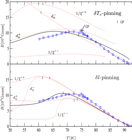
Figure 4: The BG-VG, BG-VL first-order transition lines $B_{m}(T)$ given in (103) for $\delta T_{c}$-pinning (upper figure) and $\delta l$-pinning (lower figure). The solid lines are calculated with parameters for $d_{0}$ and $\xi^{\prime}$ which gives one of the best fits to the experimentally determined Bouquet1 BG-VL line (square points) within the pinning mechanism ($2\pi d_{0}\,\xi_{ab}^{2}/{\xi^{\prime}}^{2}=1.5\cdot 10^{-7}$ and $\xi_{ab}/\xi^{\prime}=1.59$ for $\delta T_{c}$-pinning, $2\pi d_{0}\,\xi_{ab}^{2}/{\xi^{\prime}}^{2}=1.32\cdot 10^{-6}$ and $\xi_{ab}/\xi^{\prime}=1.49$ for $\delta l$-pinning). Dotted curves are calculated by a variation of these parameters given by $d^{\pm}_{0}=(1\pm 1/2)d_{0}$ and $1/{\xi^{\prime}}^{\pm}=(1\pm 1/2)^{1/2}/\xi^{\prime}$ where only one parameter was varied. We wrote that parameter at the curve. The vertical markers denote the intersection points of the glass transition line and the BG-VG, BG-VL line named GP. From Clausius-Clapeyron equation (107) the critical points CPs are determined by an extremum of the BG-VG, BG-VL lines

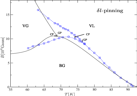
Figure 5: Phase diagram for YBCO. Solid lines represent the theoretical determined phase transition lines between the various phases calculated for $\delta l$-pinning with $2\pi d_{0}\,\xi_{ab}^{2}/{\xi^{\prime}}^{2}=1.32\cdot 10^{-6}$ and $\xi_{ab}/\xi^{\prime}=1.49$ corresponding to the solid line in the lower picture in Fig. 4. The glass transition line VG-VL was calculated from (104). Square points represent the experimentally determined phase diagram of Bouquet et al. Bouquet1 .

As derived in section VIB, the glass transition line which is the border of the replica symmetric solution of the Mézard-Parisi variational calculation and the one-step replica symmetry-breaking solution, where the stabilities was discussed in section VII, is determined by $m_{1}=1$ in (63) resulting in

$${\cal D}_{\infty}(0)A_{\infty}=1\qquad({\rm VG-VL\;line}).$$ (104)

This equation corresponds to the depinning temperature $T_{\rm dp}$ of a one-dimensional string in three dimensions in a random environment Blatter1 . The Larkin length $L_{c}$ is defined by the length where we have a coherently pinning of the string which means $u^{2}(0,L_{c})=\xi^{\prime 2}\sim\xi^{2}_{ab}$ with

$$u^{2}(L,L_{3})\equiv\overline{\langle({\rm u}(L,L_{3})-{\rm u}(0,0))^{2}\rangle}\,.$$ (105)

When temperature fluctuations become larger there is a softening of the impurity potential which is important for the length of the coherently pinned vortices. This correction is important when this fluctuation length becomes equal to $L_{c}$ calculated for $T=0$. This depinning temperature is given by (104) Blatter1 . We mention that it is difficult to distinguish experimentally by diffraction experiments in which of the two classes $\kappa_{1}[K]>1-17/6A_{\infty}^{2}$ or $\kappa_{1}[K]\leq 1-20/6A_{\infty}^{2}$ the disorder correlation potential $K$ of a given experiment belongs. In both regimes we obtain $u^{2}(0,L_{3})\propto(k_{B}T)L_{3}/c_{44}a^{2}$ in the VG-VL phase (the proportionality constant is different for both regimes, see also the discussion in Appendix A). This is reasoned in the vanishing support of $\sigma(s)$ in the vicinity of the origin, fact for the the one-step replica symmetry-breaking regime $\kappa_{1}[K]\leq 1-20/6A_{\infty}^{2}$ (58) as well as the continuous replica symmetry-breaking regime $\kappa_{1}[K]>1-17/6A_{\infty}^{2}$ (70) and (75). It means that thermal fluctuations are dominant over disorder fluctuations. Note that $u^{2}(L,L_{3})$ for $L\not=0$ diverges in the VG as well as the VL phase characteristic for defect dominated phases also seen before for the system without disorder. For the BG-phase in the random manifold regime we obtain $u^{2}(L,L_{3})\propto(L^{2}+L^{2}_{3})^{1/6}$ in accordance with former calculations Giamarchi1 . The derivation beyond the random manifold regime where the lattice structure is important leads to $u^{2}(L,L_{3})\propto\log(L^{2}+L^{2}_{3})$ Giamarchi1 .

Mikitik and Brandt found in Ref. Mikitik1, ; Mikitik2, that their analytical derived BG-VG, BG-VL curve is a function of the Ginzburg number ${\rm Gi}=32\pi^{4}(\lambda_{ab}(0)\lambda_{c}(0)T_{c}/\phi_{0}^{2}\xi_{ab}(0))^{2}$, $b$, $T/T_{c}$, and the disorder function ${\cal D}(0)$. This can be also shown easily for the melting curve (103). Note that the disorder constant $D$ in Ref. Mikitik1, ; Mikitik2, is a function of $b$, $T/T_{c}$, ${\rm Gi}$ and our disorder function ${\cal D}(0)$.

In Fig. 4 we show the BG-VG, BG-VL curves given by (103) for various values $d_{0}$, $\xi^{\prime}$. The upper curves are calculated with a $\delta T_{c}$-pinning correlation function (10), the lower curves for a $\delta l$-pinning impurity correlation function (11). For clearance we do not show the critical points CP on the melting line in the figure which are characterized by zero entropy jumps $\Delta S_{l}$ per double layer and vortex over the transition line. These points can be easily marked in the figure since they correspond to the extrema of the melting line $B_{m}$ due to the Clausius-Clapeyron equation given in (107) below.

The intersection point of the glass transition line BG-VL which is calculated by (104) with the BG-VG, BG-VL line is denoted by GP in the figure. The square points with the dashed line denotes the experimentally determined BG-VG, BG-VL line of Bouquet et al. Bouquet1 shown also in Fig. 2 for comparison. In the $\delta T_{c}$ part of the figure, we find no solutions for the equation (103) near $T\approx T_{c}$. The parameters of the straight lines in the figure are chosen in such a way that we reproduce in one of the best ways the form of the experimentally melting line of Bouquet et al. Bouquet1 and also the position of the experimentally found CP and GP. These experimentally chosen parameters are $2\pi d_{0}\,\xi_{ab}^{2}/{\xi^{\prime}}^{2}=1.32\cdot 10^{-6}$ and $\xi_{ab}/\xi^{\prime}=1.49$ for $\delta l$-pinning, $2\pi d_{0}\,\xi_{ab}^{2}/{\xi^{\prime}}^{2}=1.5\cdot 10^{-7}$ and $\xi_{ab}/\xi^{\prime}=1.59$ for $\delta T_{c}$-pinning. Thus, we obtain that the correlation length $\xi^{\prime}$ of the disorder potential almost corresponds to the coherence length $\xi_{ab}$ of the superconductor. The reason that $\xi_{ab}/\xi^{\prime}$ is larger than one could be due to lattice influences on the effective broadening of the vortex (see the notes below (11)). Finally, we mention the similarity of the $d_{0}$ parameter values in the Parisi case and the corresponding values in the quadratic disorder case of Section IV.

The curves of representative variations of these almost optimal parameter values are shown by the dotted curves. We obtain from the figure as was also the case in the second-order perturbative discussion in Section IV that the $\delta T_{c}$-pinning curves fits less to the experiment than the $\delta l$-pinning curves. This comes mainly from the smoothness of the disorder parameter $d(T)$ in (11) as a function of $T$ resulting in the slow variation of the transition line $B_{m}(T)$ seen in the upper part of Fig. 4. From Fig. 4 we obtain that the glass intersection point GP and the critical point CP does in generally not coincide. This was just mentioned in Ref. Beidenkopf1, for BSCCO where in the experiments this difference is not seen yet maybe because of experimental uncertainties.

One of the most interesting results of our calculation is that the reentrant behavior of the melting line and the experimentally not seen low $B$ parts of the BG-VG curves in the quadratic disorder calculation of section IV (see Figs. 2 and 3) vanished in the Parisi approach. It is remarkably that the large descend of the curves in the direction to lower temperatures in Fig. 2 within the quadratic approach are smoothed within the Mézard-Parisi approach such that the BG-VG transition curves is almost horizontal. There are various forms of the BG-VG lines in the literature. One of the reasons of the differences in the various experiments comes presumably from the strong dependence of the BG-VG line on the depinning function $d(T)$ via an exponential behavior in (103). Any perturbational effects like surface effects or twinning areas in the crystal can change the functional form of the curve at small temperatures easily. We note that especially the strong dependence of the BG-VG curve on small variations of the disorder correlation length $\xi^{\prime}$ having its reason in the quadratic dependence of $\xi^{\prime}$ in $A$ (65) which is contained as a third-order summand in the free energy of the solid phase in (100). The form of the free energy in the solid phase is the most dominant factor for the form of the BG-VG curve in the vicinity of the critical point CP. This is in contrast to the free energy in the high-temperature phase which just grows in importance beyond the glass intersection point GP but is still small compared to the free energy part of the solid phase.

In Fig. 5 we show the whole phase diagram for the parameters of the solid curve in the lower $\delta l$-pinning part of Fig. 4 (solid curve). For comparison (square points with dashed curve) we show also the experimentally determined phase diagram of Bouquet et al. of Ref. Bouquet1, . Both phase diagrams look rather similar except that the CP and GP points of the theoretical determined phase diagram lies a little bit lower in temperature in comparison to the experimental ones. The upper curve between the VG-VL phases show the glass transition line calculated by (104). There is a small discrepancy in the slope of the line between theory and experiment. Note that for $\tilde{\lambda}\approx\lambda$ which is the case for BSCCO Brandt1 we get that ${\cal D}_{\infty}(0)A_{\infty}$ is in fact independent of the magnetic field $B$ resulting in a vertical glass transition line. This is in good accordance to the experiments Beidenkopf1 .

Next, we calculate the entropy and magnetic induction jumps over the BG-VG, BG-VL first-order line. Denoting the spacing between the CuO₂ double layers by $a_{s}$ we obtain for the entropy jump per double layer and vortex over the BG-VG, BG-VL line

$$\Delta S_{l}\approx k_{B}T_{m}\frac{a_{s}}{a_{3}}\frac{\partial}{\partial T_{m}}\,\ln[Z^{T\to\infty}_{\rm fl}/Z^{T\to 0}_{\rm fl}]$$ (106)

and a corresponding equation for the glass transition line. Now we make use of the Clausius-Clapeyron equation which relates the jump of the entropy density of a first-order transition line to the jump of the magnetic induction by

$$\frac{a_{3}\Delta S_{l}}{va_{s}}=-\frac{dH_{m}}{dT}\frac{\Delta B}{4\pi}.$$ (107)

Here $H_{m}$ is the external magnetic field on the BG-VG, BG-VL line. Because $B\sim H_{c2}(T)$ for YBCO we can use $H\approx B$ in the Clausius-Clapeyron equation (107). Equation (107) is not appropriate for a numerical evaluation because of the vanishing of the denominator at the saddle points of the BG-VG, BG-VL line which are canceled due to zero points in the numerator. By using the intersection criterion for the transition line we can transform (107) to

$$\Delta B\approx k_{B}T_{m}\frac{4\pi}{v}\frac{\partial}{\partial B_{m}}\,\ln[Z^{T\to\infty}_{\rm fl}/Z^{T\to 0}_{\rm fl}]\,.$$ (108)

This equation can be also derived from thermodynamical relations under the considerations $\Delta B/B_{m}\ll 1$ which we also used by taking the intersection criterion for the free energy and not for the corresponding Gibb’s potential in this paper Tinkham1 .

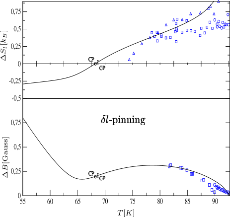
Figure 6: In the upper figure we show the entropy jump $\Delta S_{l}$ per double layer and vortex according to (106). The points in the figure are entropy jumps determined by experiments (circles Willemin1 , squares Schilling1 , triangles Bouquet1 ). In the lower figure we show the magnetic induction jumps $\Delta B$ calculated by the help of (108). Experimental points in this figure are from Ref.  Willemin1, (circles) and Ref. Welp1, (squares). The solid curves in both figures correspond to the jumps over the BG-VG, BG-VL line. We used for the whole figure parameter values $2\pi d_{0}\,\xi_{ab}^{2}/{\xi^{\prime}}^{2}=1.32\cdot 10^{-6}$ and $\xi_{ab}/\xi^{\prime}=1.49$ in correspondence to the parameter values in Fig. 5.

In Fig. 6 we show $\Delta S_{l}$ and $\Delta B$ for the parameters used in Fig. 5 over both lines. We show in the upper part of the figure $\Delta S_{l}$ with experimental points of various torque and SQUID experiments (circles Willemin1 , squares Schilling1 , triangles Bouquet1 ) for the entropy jump over the BG-VG, BG-VL line. For the parameters used in Fig. 5 we obtain a value for the CP of $68K$. In the lower part of Fig. 6 we show the magnetic induction jumps $\Delta B$. The square and circle points are experiments (circles Willemin1 , squares Welp1 ). Finally, we note that our curves of the entropy and magnetic induction jumps over the BG-VG, BG-VL line is in qualitative agreement with similar curves calculated within the Ginzburg-Landau approach for YBCO by Li and Rosenstein Li1 . The main difference is that they obtain a zero point in the magnetic induction jump curve in the vicinity of the critical point which has its reason in the reentrant behavior of their calculated melting line to second order in the disorder potential (see (107) by taking into account that $dB_{m}/dT$ is infinite at the reentrant points). We expect, as was also the case in the elasticity approach used here, that this zero point vanishes when going beyond second-order perturbation theory leading to the vanishing of the reentrant behavior.

Finally, we come back to a discussion of the scenarios of the phase diagram for YBCO given in the introduction of this paper. We did not find a slush phase within our numerical examinations of equation (103) during this work irrespective of the parameter range. This in accordance to the Ginzburg-Landau calculations of Li and Rosenstein in Ref.  Li1, . This means that our phase diagram is only in accordance with the second scenario of a unified BG-VG, BG-VL first-order line discussed in the introduction of this paper. Due to the controversy of this phase we cannot determine within our theoretical approach whether it is in fact existent or not. It was claimed in the experimental paper Nishizaki1 that the slush phase only exists within a really small doping region where the entropy jumps over the first-order line between the slush phase VS and the vortex liquid VL is two orders smaller than the entropy jumps over the BG-VL melting line. The intersection criterion of the high and low-temperature free energy used in this paper by a perturbative calculation in both phases uses the assumption that the slope difference corresponding to the entropy jumps is not too small. This could be the reason that we do not see the slush phase. We point out that to our knowledge there exist no theoretical model which shows without doubt the existence of this phase.

One of the main findings in this work for vortex model (2) is that the order of the glass transition VG-VL is of third order irrespective of the form of the disorder correlation potential. We point out that a third order phase transition having a smooth heat capacity should show scaling behavior with a non-trivial fix point in a renormalization group calculation. Prominent examples of third order phase transitions is the non-interacting homogeneous three dimensional Bose gas across the Bose Einstein transition Junod1 or the large $N^{\prime}$-limit of the two dimensional $U(N^{\prime})$ lattice gauge theory with a variation in the coupling constant Gross1 . It was noticed in Ref. Junod1 that the heat capacity curves for BSCCO over the superconducting transition without magnetic field looks rather similar to the heat capacity curves of the homogeneous Bose gas. For YBCO this transition looks more like the $\lambda$-transition of ⁴He. A discussion of scaling relations in higher order phase transitions and their classification due to Ehrenfest can be found in Ref. Kumar1, .

Fisher et al. proposed in Ref. Fisher1, a scaling behavior of the VG-VL glass transition where they introduce a disorder phase correlation length $\xi_{G}$ with scaling $\xi_{G}\sim|T-T_{G}|^{-\nu}$ in the fluid phase near glass transition temperature $T_{G}$ on the VG-VL transition line. This scaling proposal was later on approved experimentally via measurements of the current voltage characteristics over the transition region Gammel1 . There are now a number of experiments Gammel1 ; Klein1 and computer simulations Reger1 ; Lidmar1 ; Kawamura1 of various models for superconductors showing also this scaling behavior where in most cases the disorder phase correlation exponent lies in between $0.8\leq\nu\leq 1.7$. One can connect the phase correlation scaling exponent $\nu$ with the heat capacity exponent $\alpha$ defined by $C\sim|T-T_{G}|^{-\alpha}$ where $C$ is the heat capacity via the hyperscaling relation $\nu d=2-\alpha$. Here $d$ is the dimension of the system which means $d=3$ in our case. Thus, most of the experimentally determined and computer simulated systems have an $\alpha$-exponent lying in between $-3.1\leq\alpha\leq-0.4$. This corresponds to a phase transition of order three or even higher within the Ehrenfest definition of phase transitions Kumar1 .

X Summary

In this paper, we have derived the phase diagram for superconductors having their phase transition lines at high magnetic fields near $H_{c2}$, such as YBCO. The aim was to obtain a unified analytic theory for the BG-VG, BG-VL transition as well as for the glass transition lines. The model consists of the elastic degrees of freedom of the vortices with additional defect fields describing in the most simple way the defect degrees of freedom of the vortex lattice. For the impurity potential we restricted us to weak pinning $\delta T_{c}$ and $\delta l$-correlated impurities Blatter1 .

First, we have derived the effective low- (14) and high-temperature Hamiltonians (15) without disorder in Section III. The low-temperature Hamiltonian consist of the well-known elastic Hamiltonian of a vortex lattice where defects are frozen out. At high-temperatures, the stress fields are frozen out leading to the high-temperature Hamiltonian (15). In Section IV we have carried out the disorder averaging to second-order perturbation theory with these low- and high-temperature Hamiltonians to find the BG-VG, BG-VL transition line by the application of the intersection criterion. The result given in Eq. (31) and displayed in Fig. 2 shows a reentrant behavior. The low-${B}$ behavior of the calculated transition line was not in agreement with experiment. This led us to calculate the free energy in the low- and high-temperature phases using the non-perturbative approach of Mézard-Parisi. In Section VI we calculated the variational free energy in the high-temperature liquid phase. We obtain a glass transition from a replica symmetric solution corresponding to the vortex liquid VL to a symmetry broken solution corresponding to the vortex glass phase VG. The position of the glass transition line fulfills equation (104) describing the depinning transition of a string with stiffness $c_{44}a^{2}$ in three dimensions. The degree of replica symmetry breaking of the variational Hamiltonian depends on the form of the disorder correlation function. The high-temperature part of the free energy is given by (102). For high magnetic fields near $H_{c2}$ we got the following result: We obtain a one-step replica symmetry-breaking solution when the kurtosis $\kappa_{1}$ of the disorder correlation function in position space defined in (87) is smaller than one. In the case that the kurtosis is larger than or equal to one we obtain a full replica symmetry broken solution. In both cases we obtain a third order glass transition line. The Gaussian correlation function is the border in the disorder correlation function space with $\kappa_{1}=1$. Corrections to this simple rule relevant for lower magnetic fields are given in Table 1.

In Section VIII, we calculate the free energy of the vortex system in the low-temperature solid phase (BG), given by (101). The stationary solution for the self-energy matrix in replica space is continuous replica symmetry broken. By using the intersection criterion for the low- and high-temperature free energies, we calculate the expression for the unified BG-VG, BG-VL line given by (103). In Fig. 4 we show the unified BG-VG, BG-VL line for various parameters for both pinning mechanisms. We obtain that $\delta l$-pinning fits much better to the experiments than $\delta T_{c}$-pinning. It is seen that the reentrant behavior of the second-order perturbation theory carried out in Section III vanished in this non-perturbative approach. In Fig. 5, we show the theoretical determined phase diagram for YBCO. Fig. 6 shows the entropy jumps and magnetic field jumps over the BG-VG, BG-VL transition line. Finally, we calculated heat capacity scaling exponents $\alpha$ from disorder phase correlation exponents $\nu$ determined from experiments and computer simulations via the hypercaling relation across the glass transition line VG-VL which is only consistent with a third or even higher order VG-VL phase transition line.

Appendix A Justifications for approximation of disorder Hamiltonian (42)

We restrict us here to the case of transversal fluctuation where the generalization to arbritrary fluctuations is straight forward. That (42) is valid for the high-temperature fluid phase was shown below (45).

In the solid phase, we first have to show that $k_{B}T\,2\,|G^{T}_{s}(a{e}_{i})-G^{T}_{s}(0)|/v\ll a^{2}$ in the interesting regime near the melting line where $G^{T}_{s}$ is the full Green function. $a{\bf e}_{i}$ is a nearest neighbor vector in the xy-plane and $s$ is a continuous Parisi index. It follows from Mezard1

$$G^{T}_{s}({\bf x})=\frac{1}{V_{\rm BZ}}\int_{\rm BZ}d^{2}kdk_{3}\;e^{i{\bf k}\cdot{\bf x}}\;G_{0}^{T}$$ (109)

$$\times\left[\frac{1}{s}\frac{\Delta(s)}{({G_{0}^{T}})^{-1}+\Delta(s)}+\int_{0}^{s}\frac{ds}{s^{2}}\frac{\Delta(s)}{({G_{0}^{T}})^{-1}+\Delta(s)}\right]$$

that the nearest neighbor fluctuations are in fact much smaller than the nearest neighbor distance $a$ when taking into account (95), (99), $c^{2}_{L}\ll 1$ and $D(A)A\lesssim 1$ near the melting and glass line which is the regime we are interested in.

Finally, we have to show that $B(\Delta(s))\ll a^{2}$ for almost all $s>0$. From (51), (99) with (95), $c_{L}^{2}\ll 1$ and $D(0)A\lesssim 1$ we obtain $B(\Delta(s))\ll a^{2}$ for

$$s\gg c_{L}^{8}\,.$$ (110)

which is almost the whole $s$-region. The extreme small range $s\ll c_{L}^{8}$ has no relevance for the free energy result. As mentioned above, this small $s$-region of $\sigma(s)$ becomes relevant only when calculating disorder fluctuations (105) beyond the random manifold regime which corresponds to distances $L$, $L_{3}$ where $u^{2}(L,L_{3})\gg a^{2}$ Giamarchi1 .

Appendix B Stability of Mézard-Parisi solutions

In this section, we consider the stability criterion of the Mézard-Parisi theory in the large $N^{\prime}$-limit and in the Bogoliubov variational method. First, we reconsider the derivations of Carlucci et al. Carlucci1 for the stability conditions in the case of the large $N^{\prime}$-limit. Then we derive the corresponding stability criteria in the variational approach considered in Section VI. To our knowledge this was not done before in the literature.

In order to compare the vortex lattice theory with two component displacement fields with the $N^{\prime}=2$ isotropic random manifold theory of Mézard and Parisi we restrict us in the following first to the transversal displacement fields justified above as a good approximation in both phases. A generalization to the full fluctuations is straight forward. The difference of the stationary and stability expressions in both phases for the vortex lattice and the isotropic $N^{\prime}=2$ random manifold theory of Mézard and Parisi comes then mainly due to a difference in the kinetic part of the Hamiltonian $G_{0}^{-1}$ in Eq. (41). As was shown in Ref. Mezard1, the saddle point equation of both approaches looks rather similar except that in the large $N^{\prime}$-limit the saddle point equation (52), ${\cal D}_{0}(x)$ should be replaced by $f(x)$ where $f(x)=\Delta(\sqrt{x})/(K_{B}T)^{2}$ (we take the reversed sign to the Mézard-Parisi definition). $\Delta(\sqrt{x})$ is the impurity correlation function in (34). To derive this, Mézard and Parisi insert in the action of the isotropic random manifold system, auxiliary fields. By integrating out the fluctuating displacement fields of the random manifold the large $N^{\prime}$-limit corresponds to a saddle point approximation in the auxiliary fields. This results in the saddle point equation (34). By the definition of

$$\tilde{f}(x)=\int_{0}^{\infty}d\alpha\;e^{-\alpha}f(\alpha x)$$ (111)

Mézard and Parisi obtain (52) for the general variational approach where the disorder function ${\cal D}_{0}(x)$ is replaced by $\tilde{f}(x)$.

B.1 Stability in the large $N^{\prime}$-limit approach of Mézard and Parisi

The stability of the stationary solution (52) comes from the stability of the saddle point approximation of the action in the auxiliary fields. This results in the stability matrix Mezard1 (we take into account only the less stable part of the stability matrix corresponding to zero moments)

$$M^{\alpha\beta,\gamma\delta}=\frac{1}{2f^{\prime\prime}(L^{(1)}_{\alpha\beta,\alpha\beta})}\delta_{\alpha\beta,\gamma\delta}-L^{(2)}_{\alpha\beta,\gamma\delta}$$ (112)

with

$$L^{(1)}_{\alpha\beta,\gamma\delta} =\frac{(k_{B}T)}{v\,V_{\rm BZ}}\int_{\rm BZ}d^{2}kdk_{3}\;(G_{\alpha\gamma}-G_{\alpha\delta}-G_{\beta\gamma}+G_{\beta\delta})$$ (113)

$$L^{(2)}_{\alpha\beta,\gamma\delta} =\frac{(k_{B}T)^{2}}{v^{2}\,V_{\rm BZ}}\int_{\rm BZ}d^{2}kdk_{3}\;(G_{\alpha\gamma}-G_{\alpha\delta}-G_{\beta\gamma}+G_{\beta\delta})^{2}$$ (114)

and $\alpha<\beta$ and $\gamma<\delta$. Here $G_{\alpha\beta}({\bf k})$ stands for the transversal component of the Green function (41) in the case of the vortex lattice or the corresponding Green function in the case of the isotropic two component $N^{\prime}=2$ random manifold system Mezard1 . The stability of the saddle point of (40) fulfilling the discrete version of the self-energy equation (52) is given when all eigenvalues of the stability matrix (112) are positive.

$M^{\alpha\beta,\gamma\delta}$ is a four index ultrametric matrix Dotsenko1 . It was shown by Kondor et al. Kondor1 and later on by Temesvári et al. Temesvari1 that one can divide the eigenvalues of matrices of the form (112) in three classes. The first two families consist of vectors in the longitudinal sector of dimension $R+1$ and $R$ anomalous sectors of dimension $R+1$ depending explicitly on the form of the ultrametric matrix. Here, we denote $R$ by the level of hierarchy of the self-energy matrix $\sigma_{\alpha\beta}$ fulfilling the stationarity condition (52). This means $R=0$ for the replica symmetric solution calculated in section VIA and $R=1$ for the one-step solution given in section VIB for the fluid phase.

There is no closed form in the literature for the eigenvectors and eigenvalues of the matrix in (112) for the first two families. Nevertheless, it is able to block diagonalize the matrix $\underline{\rm M}$ given by (112) in the various sectors Temesvari1 . Following Temesvári et al. Temesvari1 , we denote the size of the Parisi blocks as $p_{r}$, $r=1\ldots R$, where $R$ is the maximum level of replica symmetry breaking. We denote $p_{0}=n$ and $p_{R+1}=1$, the latter being the size of diagonal elements. The matrix elements $\sigma_{\alpha\beta}$, that belong to the $r$th level of replica symmetry breaking are all equal to a number denoted by $\sigma_{r}$, $r=0,\ldots,R$. The replica overlap function is defined by $\alpha\cap\beta=r$ when $\sigma_{\alpha\beta}=\sigma_{r}$.

Denoting $u^{k}_{r}$ with $0\leq r\leq R$ the basis vectors in the first two families. For $k=0$ which is the longitudinal sector we obtain for the $R+1$ basis vectors Temesvari1

$$(u^{0}_{r})_{\alpha\beta}=\left\{\begin{array}[]{ccc}1&\mbox{for}&\alpha\cap\beta=r\,,\\ 0&\mbox{for}&\alpha\cap\beta\not=r\,.\end{array}\right.$$ (115)

The basis vectors $u^{k}_{r}$ for $k\not=0$ corresponding to the anomalous sector can be found in Ref. Temesvari1, .

The third family of eigenvectors of ultrametric matrices as for example (112) is named the replicon sector. It consist on several one-dimensional subfamilies labeled by $r=0,\ldots,R$ and $k,l=r+1,\ldots,R+1$. The corresponding one-dimensional subspaces are eigenspaces with the eigenvalues denoted by $\lambda(r;k,l)$. The eigenvectors corresponding to the basis vectors in this sector can be found in Ref. Temesvari1, . Note that these eigenvectors do not depend on the entries of the ultrametric matrix. The eigenvalues $\lambda(r;k,l)$ can be generally expressed via the matrix elements of the ultrametric matrix Temesvari1 . In the case of the concrete ultrametric matrix $\underline{\rm M}$ (112) one finds Carlucci1

$$\lambda(r;k,l)=\frac{1}{2f^{\prime\prime}(2(K_{B}T/v)(g_{R+1}-g_{r}))}-L^{\prime}_{kl}$$ (116)

with

$$L^{\prime}_{kl}=2\frac{(k_{B}T)^{2}}{v^{2}\,V_{\rm BZ}}$$ (117)

$$\times\int_{\rm BZ}d^{2}kdk_{3}\;\frac{1}{[(G_{0})^{-1}+\Delta_{l-1}]}\;\frac{1}{[(G_{0})^{-1}+\Delta_{k-1}]}\,.$$

Here $g_{k}$ corresponds to the value of the transversal component of the Green function $G_{\alpha\beta}$ (41) integrated over the momenta as in (49) or the corresponding random manifold Green function with $\alpha\cap\beta=k$. The eigenvalues $\Lambda(r;k,l)$ for $k=l=r+1$ are the most singular ones for definite $r$. One can show easily Carlucci1 that these most singular eigenvalues are zero in the case of continuous symmetry-breaking solutions as in section VIC for the fluid phase. We note that for the stability matrix sector of moments unequal to zero there are only eigenvalues larger than zero Carlucci1 .

Finally, we sketch the proof given in Ref. Carlucci1, that eigenvalues of the first two families, which is the longitudinal sector and the anomalous one, has only eigenvalues which are larger or equal to the replicon eigenvalues given above. With the definitions

$$\Delta_{r}^{k}\equiv\left\{\begin{array}[]{ccc}\frac{1}{2}(p_{r}-p_{r+1})&\mbox{for}&r<k-1\\ \frac{1}{2}(p_{k-1}-2p_{k})&\mbox{for}&r=k-1\\ p_{r}-p_{r+1}&\mbox{for}&r>k-1\,.\end{array}\right.$$ (118)

and

$$\Lambda_{k}(r)\equiv\left\{\begin{array}[]{ccc}\lambda(r;k,r+1)&\mbox{for}&k\geq r+1\\ \lambda(r;r+1,r+1)&\mbox{for}&r>k-1\,.\end{array}\right.$$ (119)

we obtain

$$\rm{det}\left(\underline{M}^{(k)}-\lambda I\right)=\prod_{r=0}^{R}\left[\Lambda_{k}(r)-\lambda\right]\rm{det}\left[I+{\underline{M}^{\prime}}^{(k)}\right]$$ (120)

with

$${M^{\prime}}^{(k)}_{rs}=K_{k}^{rs}\frac{\Delta_{s}^{k}}{2(\Lambda_{k}(s)-\lambda)}$$ (121)

where we denote ${\underline{\rm M}^{\prime}}^{(k)}$ by the matrix ${M^{\prime}}^{(k)}_{rs}$ and $K_{k}^{rs}$ is a generalized discrete Fourier transform of the ultrametric matrix $\underline{\rm M}^{(k)}$ Carlucci1 . The matrix $K_{k}^{rs}$ is denoted as the kernel for the ultrametric matrix $M^{\alpha\beta,\gamma\delta}$ which means that $M^{\alpha\beta,\gamma\delta}$ is given by $M^{(k)}_{rs}=\Lambda_{k}(r)+K_{k}^{rs}\Delta_{s}^{k}/2$ in the longitudinal or anomalous sector $k$ and $r$, $s$ runs over the basis vectors in the $k$ sector.

We point out that $K_{k}^{rs}$ can be written as

$$K_{k}^{rs}=4B_{k}({\rm max}(r,s))$$ (122)

where the function $B_{k}$ can be expressed explicitly by the Green functions $G_{s}$ Carlucci1 so does not depend on the disorder function $f$. One finds

$$B_{k}(r)<0\qquad\mbox{and}\qquad B_{k}(r+1)-B_{k}(r)>0\,.$$ (123)

Denoting $\rm{det}_{{\cal S},{\cal S}^{\prime}}[{\underline{\rm M}^{\prime}}^{(k)}]$ by the determinant of the sub-matrix of ${\underline{\rm M}^{\prime}}^{(k)}$ with lines in $\quad{\cal S}\in\{0,\ldots,R\}$ and columns in $\quad{\cal S}^{\prime}\in\{0,\ldots,R\}$ where we suppose that ${\cal S}$ and ${\cal S}^{\prime}$ has the same number of elements denoted by $\#{\cal S}^{\prime}=\#{\cal S}^{\prime}$. We obtain

$$\rm{det}\left(\underline{M}^{(k)}-\lambda I\right)=\prod_{r=0}^{R}\left[\Lambda_{k}(r)-\lambda\right]\sum_{\cal S}{\rm det}_{{\cal S},{\cal S}}[{\underline{M}^{\prime}}^{(k)}]\,.$$ (124)

In Carlucci1 it is shown that the right hand side is larger than zero for $\lambda\leq{\rm Min}_{r}[\Lambda_{k}(r)]$. This means that the eigenvalues in the non-replicon sectors are always larger than the smallest eigenvalue in the replicon sector. We now give a more general proof of this fact useful in the next subsection:

This is true if ${\rm det}_{{\cal S},{\cal S}^{\prime}}[{\underline{\rm M}^{\prime}}^{(k)}]\geq 0$ for $\quad{\cal S},{\cal S}^{\prime}\in\{0,\ldots,R\}$. We suppose the ordering $s_{i}<s_{i+1}$ for $s\in{\cal S}$ and similar for ${\cal S}^{\prime}$. By subtracting appropriate line and columns of the matrix $\underline{\rm K}_{k}$ where $\underline{\rm K}_{k}$ denotes the matrix $K^{rs}_{k}$ we obtain a matrix where its determinant is built purely from its diagonal elements given by

$${\rm det}_{{\cal S},{\cal S}^{\prime}}[\underline{\rm K}_{k}]=4^{\#{\cal S}}B_{k}({\rm max}(s_{\#{\cal S}},s^{\prime}_{\#{\cal S}^{\prime}}))$$

$$\times\prod_{i=1}^{\#{\cal S}-1}\left[B_{k}({\rm max}(s_{i},s^{\prime}_{i}))-B_{k}({\rm max}(s_{i+1},s^{\prime}_{i+1}))\right]\,.$$ (125)

By using (121) with $\Delta^{k}_{r}\leq 0$ (118) for $n\to 0$ and (123) we obtain ${\rm det}_{{\cal S},{\cal S}^{\prime}}[{\underline{\rm M}^{\prime}}^{(k)}]\geq 0$ for $\lambda\leq{\rm Min}_{r}[\Lambda_{k}(r)]$.

It is clear from the considerations above that the various sectors especially the longitudinal sector depends on the concrete hierarchical structure we choose. This means, that we can also get other eigenvalues for the various sectors by starting from a given minimal level of hierarchy by an appropriate artificial division of the various sectors leading to a larger level of hierarchy. It is clear that nevertheless the lowest eigenvalue of the stability matrix being in the replicon sector didn’t change. Now suppose, we try to restrict the stability matrix $M^{\alpha\beta,\gamma\delta}$ to the $k=0$ longitudinal sector of a suitable subdivided hierarchy, corresponding to a search of the minimum of $F_{\rm var}$ (38) in the self-energy matrices $\sigma_{\alpha\beta}$ which are contained in the Parisi-algebra.

For a subdivision of blocks we obtain that $B_{k}(r)$ given explicitly in Carlucci1 is constant on two blocks in the subdivided hierarchy originating from the same blocks $k$ and $r$ in the precursor hierarchy. Furthermore, we get doublings in the eigenvalues $\Lambda^{k}(r)$ corresponding to the subdivision. But this results to ${\rm det}_{\cal S,\cal S}[\underline{\rm M}^{(k)}]\not=0$ only if ${\cal S}$ does not contain two blocks in the subdivided hierarchy originating from the same block. Then we immediately obtain from (121), (122), (124) that we can always subdivide the hierarchy in such a way that the lowest eigenvalue in the $k=0$ longitudinal sector is given by the minimum of the eigenvalues in the replicon sector ${\rm Min}_{r}[\Lambda_{0}(r)]$. This means that by restricting the stability matrix $M^{\alpha\beta,\gamma\delta}$ to the subspace of symmetric self-energy matrices in the Parisi-algebra with the constraint (46) we obtain that the lowest eigenvalue of the restricted matrix $M^{\alpha\beta,\gamma\delta}$ is equal to the lowest eigenvalue in the replicon sector.

B.2 Stability in the variational approach of Mézard and Parisi

In this subsection, we carry out a similar analysis for the Bogoliubov variational approach of the Mézard-Parisi theory, outlined in Section IV, as was done for the large $N^{\prime}$-limit theory in the last subsection. The self-energy within this approach is calculated by searching for the stationary points of the variational free energy (37). We get a stability matrix of this stationary point by taking the second derivative of $F_{\rm var}$ with respect to the self-energy matrix under the constraint (46). This was calculated in Ref. Sasik1, . We obtain

$$\tilde{M}^{\alpha\beta,\gamma\delta} = \frac{K_{B}T}{Nv^{2}}\frac{\partial^{2}F_{\rm var}}{\partial\sigma_{\alpha\beta}\partial\sigma_{\gamma\delta}}$$

$$= \frac{1}{2}L^{(2)}_{\alpha\beta,\gamma\delta}-L^{(2)}_{\alpha\beta,\alpha^{\prime}\beta^{\prime}}\tilde{f}^{\prime\prime}(L^{(1)}_{\alpha^{\prime}\beta^{\prime},\gamma^{\prime}\delta^{\prime}})L^{(2)}_{\gamma^{\prime}\delta^{\prime},\gamma\delta}$$

This matrix corresponds to the matrix $M^{\alpha\beta,\gamma\delta}$ (112) in the large $N^{\prime}$-limit approach. Because $\tilde{M}^{\alpha\beta,\gamma\delta}$ is a ultrametric matrix we obtain by using the rather general consideration for eigenvalues in the replicon sector of these types of matrices Temesvari1

$$\tilde{\lambda}(r;k,l)=L^{\prime}_{kl}\left\{\frac{1}{2}-\tilde{f}^{\prime\prime}(2(K_{B}T/v)[g_{R+1}-g_{r})]L^{\prime}_{kl}\right\}\,.$$ (127)

By comparing (127) with (116) we obtain also in the variational approach that the most divergent eigenvalues $\tilde{\lambda}(r;r+1,r+1)$ are zero in the continuous replica symmetry-breaking solutions as was also the case in the large $N^{\prime}$-limit approach.

In the following we show that in the variational approach the eigenvalues of the longitudinal and anomalous sectors are larger than zero. We first define the reduced stability matrix

$$\underline{\tilde{\rm M}}_{\rm red}\equiv(\underline{\rm L}^{(2)})^{-1}\underline{\tilde{\rm M}}(\underline{\rm L}^{(2)})^{-1}$$ (128)

Here $\underline{\rm L}^{(2)}$ is the matrix $L^{(2)}_{\alpha\beta,\gamma\delta}$. By using that the kernel of $\underline{\rm L}^{(2)}$ is given by $-K_{k}^{rs}$ we obtain for the kernel of $(\underline{\rm L}^{(2)})^{-1}$ Carlucci1

$$\underline{\rm F}^{0}_{k}=(\underline{\Lambda}^{0}_{k})^{-1/2}(\underline{\rm N}^{0})_{k}^{-1}(\underline{\Lambda}^{0}_{k})^{-1/2}\;\underline{\rm K}_{k}(\underline{\Lambda}^{0}_{k})^{-1}$$ (129)

with

$$\underline{\rm N}^{0}_{k}={\rm I}-\frac{1}{2}(\underline{\Lambda}^{0}_{k})^{-1/2}\underline{\rm K}_{k}\underline{\Delta}^{k}(\underline{\Lambda}^{0}_{k})^{-1/2}$$ (130)

where $(\underline{\rm\Lambda}_{k}^{0})_{rs}=\Lambda^{0}_{k}(r)\,\delta_{rs}$ and $\Lambda^{0}_{k}(r)$ is given by

$$\Lambda^{0}_{k}(r)\equiv\left\{\begin{array}[]{ccc}L^{\prime}_{k,r+1}&\mbox{for}&k\geq r+1\\ L^{\prime}_{r+1,r+1}&\mbox{for}&r>k-1\,.\end{array}\right.$$ (131)

We mention that $\underline{\rm L}^{(2)}$ has positive eigenvalues which can be seen from the positivity of $G^{-1}_{\alpha\beta}$. This has to be assumed for the stability of $F_{\rm trial}$, leading to the positivity of $\underline{\rm L}^{(2)}$ for $n\to 0$ because only the first term in (B.2) is unequal to zero for $\tilde{f}=0$ where the second term in (40) does not contribute to the stability matrix Sasik1 . Now we use that $\underline{\rm L}^{(2)}$ is given by $\underline{\Lambda}^{0}_{k}-\underline{\rm K}_{k}\underline{\Delta}^{k}/2$ which means that $\underline{\rm N}^{0}_{k}$ has only positive eigenvalues. By using the same considerations for the eigenvalue equation ${\rm det}[\underline{\rm N}^{0}_{k}-\lambda]=0$ as was done at the end of the last subsection we obtain further that all eigenvalues of $\underline{\rm N}^{0}_{k}$ are lower than one. This leads to the fact that the denominator $(\underline{\rm N}^{0}_{k})^{-1}$ in $\underline{\rm F}^{0}_{k}$ (129) can be expanded in a geometric series.

The eigenvalue equation for $\underline{\tilde{\rm M}}_{\rm red}$ is given by the right hand side of Eq. (120) with $K_{k}^{rs}$ in (121) is substituted by the expanded form of $(F_{k}^{0})^{rs}$ (129). $\Lambda_{k}(r)$ is built of the replicon eigenvalues of $\underline{\tilde{\rm M}}_{\rm red}$ corresponding to (119). By carrying out the calculation of the resulting sub-determinants of sums and products of matrices by standard rules (Cauchy-Binet formula) we obtain as in the last subsection that the non-replicon eigenvalues of $\underline{\tilde{\rm M}}_{\rm red}$ are larger than the smallest replicon eigenvalue given in (127).

Furthermore, we obtain also with a similar proof as in subsection 1 that the projected matrix $\tilde{M}^{\alpha\beta,\gamma\delta}_{\rm red}$ to the space of the symmetric self-energy matrices $\sigma_{\alpha\beta}$ of the Parisi form with the constraint (46) contains the smallest replicon eigenvalue.

Up to now, we have only shown that the results of the large $N^{\prime}$ approach considered in the last subsection are also valid for the reduced stability matrix $\tilde{M}^{\alpha\beta,\gamma\delta}_{\rm red}$. It is not clear whether this is also valid for the full stability matrix $\tilde{M}^{\alpha\beta,\gamma\delta}$ (B.2) of the Mézard-Parisi variational approach. Nevertheless, one normally does not need the results above in their general form for a stability analysis of saddle point solutions of (38). It is enough for this analysis to know the results concerning the positivity of the eigenvalues. This can be immediately reached by using the defining equation (128) of the reduced stability matrix and the general conclusions above.

This leads to the following results for the stabilities in the large $N^{\prime}$ and the variational approach of the Mézard-Parisi theory:

1. The eigenvalues in the replicon sector are given by $\lambda(r;k,l)$ in (116) for the large $N^{\prime}$-approach and by $\tilde{\lambda}(r;k,l)$ in (127) for the variational approach. In the case that the eigenvalues in the replicon sector are all positive in the large $N^{\prime}$-approach or the variational approach we obtain also that all eigenvalues of the full stability matrices $M^{\alpha\beta,\gamma\delta}$ or $\tilde{M}^{\alpha\beta,\gamma\delta}$, respectively, are larger than zero. This leads to the stability of the corresponding saddle point solution.

2. The eigenvalues of the continuous symmetry-breaking solution are larger than or equal to zero.

3. The eigenvalues of the stability matrix projected on the subspace of variations in the symmetric self-energy matrices $\sigma_{\alpha\beta}$ in the Parisi algebra with the constraint (46) are larger than or equal to zero if and only if the eigenvalues of the full stability matrix not restricted to variations in the Parisi algebra in both approaches are larger than or equal to zero.
   

We further note that the eigenvalues $\lambda(r;k,l)$ (116) and $\tilde{\lambda}(r;k,l)$ (127) of both approaches are proportional to each other with a positive proportional constant when neglecting the distinction in the effective disorder functions $f$ and $\tilde{f}$ related by (111).

Appendix C Instability of finite-step replica symmetry-breaking solutions in the fluid phase

In this section we show in general that finite-step replica symmetry-breaking solutions for the fluid phase of the vortex lattice with a Gaussian disorder correlation function (12) are not stable. This will be shown irrespective of the number of steps. We have shown this in the case of one-step replica symmetry breaking in Section VI. From (47) and (60) we obtain in the case of a $R$-step replica symmetry-breaking solution in the fluid phase

$$\Delta f_{\rm var}=\displaystyle\frac{k_{B}T}{2}\sum_{i=1}^{R}\bigg{\{}\left[\frac{1}{m_{i+1}}-\frac{1}{m_{i}}\right]S(\tilde{\Delta}_{m_{i}})$$

$$+[m_{i+1}-m_{i}]\;D(\,2B[\Delta_{m_{i}}])\bigg{\}}$$ (132)

with

$$S(x) = \frac{1}{2}\left[4\rm{arcsinh}\left(\frac{x^{1/2}}{2}\right)-\frac{x^{1/2}}{(1+x/4)^{1/2}}\right]\,,$$ (133)

$$B[\Delta_{m_{i}}] = \frac{k_{B}T}{v}\bigg{\{}\sum_{j=i}^{R-1}\frac{1}{m_{j+1}}\left[g(\Delta_{m_{j}})-g(\Delta_{m_{j+1}})\right]$$ (134)

$$+g(\Delta_{R})\bigg{\}}\,.$$

In (132) we used that $\Delta_{0}=0$ and $m_{R+1}\equiv 1$. The $R$ stationarity conditions $\partial\Delta f_{\rm var}/\partial\Delta_{i}=0$ for $i=1\ldots R$ lead to

$$\sum_{i=1}^{l}\frac{\Delta_{m_{i}}\!-\!\Delta_{m_{i-1}}}{m_{i}}\!=\!-2\frac{k_{B}T}{v}D^{\prime}(2B[\Delta_{m_{l}}]).$$ (135)

for $l=1\ldots R$ corresponding to (61) in the case of the one-step replica symmetry-breaking solution. The saddle point conditions $\partial\Delta f_{\rm var}/\partial m_{i}=0$ for $i=1\ldots R$ lead to

$$\sum_{i=1}^{l}\frac{1}{m^{2}_{i}}\left[S(\tilde{\Delta}_{m_{i}})-S(\tilde{\Delta}_{m_{i-1}})\right]={\cal D}(\,2B[\Delta_{m_{l}}])-Z_{l}$$ (136)

for $l=1,\ldots,R$ with

$$Z_{l} = -\sum_{j=1}^{l}\sum_{i=1}^{j-1}\frac{\Delta_{m_{i}}}{m_{j}}\left(\frac{1}{m_{i}}-\frac{1}{m_{i+1}}\right)$$ (137)

$$\times\left[g(\Delta_{m_{j}})-g(\Delta_{m_{j-1}})\right]\geq 0\,.$$

One should compare this equation with (62) in the case of a one-step replica symmetry-breaking solution. Since $Z_{1}=0$ we can use (135) and (136) similarly as in the derivation of (83) to obtain $\tilde{\lambda}(1;2,2)<0$ irrespective of the number $R$ of hierarchical steps for $\Delta_{1}>0$. Furthermore, we obtain $\tilde{\lambda}(1;2,2)=0$ at $\Delta_{1}=0$ as was also the case in the one-step hierarchical symmetry-breaking case.

References

- (1) G. Blatter, M. V. Feigel’man, V. Geshkenbein, A. Larkin, and V. M. Vinokur, Rev. Mod. Phys. 66, 1125 (1994)
- (2) T. Nattermann and S. Scheidl, Advances in Physics 49, 607 (2000).
- (3) N. Avraham, B. Khaykovich, Y, Myasoedov, M. Rappaport, H. Shtrikman, D. E. Feldman, T. Tamegai, P. H. Kes, M. Li, M. Konczykowski, K. van der Beek , E. Zeldov, Nature (London) 411, 451 (2001).
- (4) C. J. van der Beek, S. Colson, M. V. Indenbom, and M. Konczykowski, Phys. Rev. Lett. 84, 4196 (2000).
- (5) Y. Radzyner, S. B. Roy, D. Giller, Y. Wolfus, A. Shaulov, P. Chaddah, and Y. Yeshurun, Phys. Rev. B 61, 14362 (2000).
- (6) F. Bouquet, C. Marcenat, E. Steep, R. Calemczuk, W. K. Kwok, U. Welp, G. W. Crabtree, R. A. Fisher, N. E. Phillips, A. Schilling, Nature (London) 411, 448 (2001).
- (7) D. Pal, S. Ramakrishnan, and A. K. Grover, D. Dasgupta, B. K. Sarma, Phys. Rev. B 63, 132505 (2000).
- (8) K. Shibata, T. Nishizaki, T. Sasaki, and N. Kobayashi, Phys. Rev. B 66, 214518 (2002).
- (9) M. P. A. Fisher, Phys. Rev. Lett. 62, 1415 (1989); D. S. Fisher, M. P. A. Fisher, and D. A. Huse, Phys. Rev. B 43, 130 (1991).
- (10) P. L. Gammel, L. F. Schneemeyer, and D. J. Bishop, Phys. Rev. Lett. 66, 953 (1991).
- (11) C. Reichhardt, A. vanOtterlo, and G. T. Zimányi, Phys. Rev. Lett. 84, 1994 (2000).
- (12) T. Nishizaki, T. Naito, and N. Kobayashi, Phys. Rev. B 58, 11169 (1998).
- (13) H. Beidenkopf, N. Avraham, Y. Myasoedov, H. Shtrikman, E. Zeldov, B. Rosenstein, E. H. Brandt and T. Tamegai, Phys. Rev. Lett. 95, 257004 (2005).
- (14) A. van Otterlo, R. T. Scalettar, and G. T. Zimanyi, Phys. Rev. Lett. 81, 1497 (1998).
- (15) P. Olsson and S. Teitel, Phys. Rev. Lett. 87, 137001 (2001);
- (16) J. P. Rodriguez, Phys. Rev. B 69, 100503(R) (2004).
- (17) Y. Nonomura and X. Hu, Phys. Rev. Lett. 86, 5140 (2001).
- (18) P. Olsson and S. Teitel, Phys. Rev. Lett. 94, 219703 (2005); Y. Nonomura and X. Hu, Phys. Rev. Lett. 94, 219704 (2005).
- (19) J. Lidmar, Phys. Rev. Lett. 91, 097001 (2003).
- (20) D. Li and B. Rosenstein, Phys. Rev. Lett. 90, 167004 (2003).
- (21) D. Ertaş and D. R. Nelson, Physica C 272, 79 (1996).
- (22) T. Giamarchi and P. LeDoussal, Phys. Rev. B 55, 6577 (1997).
- (23) G. P. Mikitik and E. H. Brandt, Phys. Rev. B 64, 184514 (2001).
- (24) G. P. Mikitik and E. H. Brandt, Phys. Rev. B 68, 054509 (2003).
- (25) G. I. Menon, Phys. Rev. B 65, 104527 (2001).
- (26) Y. Radzyner, A. Shaulov,Y. Yeshurun, Phys. Rev. B 65, 100513(R) (2002).
- (27) J. Kierfeld and V. Vinokur, Phys. Rev. B 69, 024501 (2004).
- (28) J. Kierfeld and V. Vinokur, Phys. Rev. B 61 R14928 (2000).
- (29) D. Li and B. Rosenstein, preprint cond-mat/0411096.
- (30) H. Kleinert, Gauge Fields in Condensed Matter, Vol. II Stresses and Defects, World Scientific, Singapore, 1989. (readable online at www.physik.fu-berlin.de/~kleinert/re.html#b2)
- (31) J. Dietel and H. Kleinert, Phys. Rev. B 73, 024113 (2006).
- (32) J. Dietel and H. Kleinert, Phys. Rev. B 74, 024515 (2006).
- (33) T. Halpin-Healy and Y. C. Zhang, Phys. Rep. 254, 215 (1995).
- (34) D. A. Gorokhov and G. Blatter, Phys. Rev. B 62, 14032.
- (35) S. Kamal, D. A. Bonn, N. Goldenfeld, P. J. Hirschfeld, R. Liang, and W. N. Hardy, Phys. Rev. Lett. 73, 1845 (1994).
- (36) M. Mézard and G. Parisi, J. Phys. I 1, 809 (1991).
- (37) V. Dotsenko, The theory of spin glasses and neural networks, Worlds Scientific, Singapore, 1989.
- (38) S. E. Korshunov, Phys. Rev. B 48, 3969 (1993).
- (39) T. Giamarchi and P. LeDoussal, Phys. Rev. Lett. 72, 1530 (1994); Phys. Rev. B 52, 1242 (1995).
- (40) D. M. Carlucci, C. De Dominicis, and T. Temesvari, J. Phys. I France 6, 1031 (1996).
- (41) E. H. Brandt, Rep. Prog. Phys. 58, 1465 (1995).
- (42) R. Labusch, Physics Letters 22, 9 (1966).
- (43) M. C. Marchetti and D. R. Nelson, Phys. Rev. B 41, 1910 (1990).
- (44) D. Stamopoulos, M. Pissas, and A. Bondarenko, Phys. Rev. B 66, 214521 (2002).
- (45) K. Deligiannis, P. A. J. de Groot, M. Oussena, S. Pinfold, R. Langan, R. Gagnon, and L. Taillefer, Phys. Rev. Lett. 79, 2121 (1997).
- (46) R. Griessen, WenHai-hu, A. J. J. van Dalen, B. Dam, J. Rector, H. G. Schnack, S. Libbrecht, E. Osquiguil, and Y. Bruynseraede, Phys. Rev. Lett. 72, 1910 (1994); D. Giller, , A. Shaulov, Y. Yeshurun, and J. Giapintzakis, Phys. Rev. B 60, 106 (1999).
- (47) L. Miu, Phys. Rev. B 65, 096501 (2002); D. Pal, S. Ramakrishnan, and A. K. Grover, Rev. B 65, 096502 (2002).
- (48) S. F. Edwards and P. W. Anderson, J. Phys. France 5, 965 (1975).
- (49) J. D. Reger, T. A. Tokuyasu, A. P. Young and M. P. A. Fisher, Phys. Rev. B 44, 7147 (1991).
- (50) M. Mézard, G. Parisi, and M. Viasoro, Spin Glass Theory and Beyond (World Scientific, Singapore, 1987).
- (51) D. B. Saakian and Th. M. Nieuwenhuizen, J. Phys. I France 7, 1513 (1997).
- (52) T. Temesvári, C. De Dominicis and I. Kondor, J. Phys. A:Math. Gen. 27, 7569 (1994).
- (53) R. Šášik, Phys. Rev. B 60, 7196 (1999).
- (54) M. Tinkham, Introduction to Superconductivity, McGraw-Hill, New York, 1996.
- (55) M. Willemin, A. Schilling, H. Keller, C. Rossel, J. Hofer, U. Welp, W. K. Kwok, R. J. Olsson, and G. W. Crabtree, Phys. Rev. Lett. 81, 4236 (1998).
- (56) A. Schilling, R. A. Fisher, and G. W. Crabtree, Nature (London) 382, 791 (1996).
- (57) U. Welp, J. A. Fendrich, W. K. Kwok, G. W. Crabtree, and B. W. Veal, Phys. Rev. Lett. 76, 4809 (1996).
- (58) A. Junod, A. Erb, and C. Renner, Physica C 317, 333 (1999).
- (59) D. J. Gross and E. Witten, Phys. Rev. D 21, 446 (1980).
- (60) P. Kumar and A. Saxena, Phil. Mag. B 82, 1201 (2002).
- (61) T. Klein, A. Conde-Gallardo, J. Marcus, C. Escribe-Filippini, P. Samuely, P. Szabo, and A. G. M. Jansen, Phys. Rev. B 58, 12411 (1998); A. M. Petrean, L M. Paulius, W. -K. Kwok, J. A. Fendrich, and G. W.Crabtree, Phys. Rev. Lett. 84, 5852 (2000).
- (62) H. Kawamura, Phys. Rev. B 68, 220502(R) (2003); H. G. Katzgraber and I. A. Campbell, Phys. Rev. B 69, 094413 (2004).
- (63) I. Kondor, C. De. Dominicis, Europhys. Lett. 2, 617 (1986).