Is it possible to experimentally verify the fluctuation relation?
A review of theoretical motivations and numerical evidence

Foreword

The statistical mechanics of nonequilibrium stationary states of dissipative systems and, in particular, the large deviations of some specific observables attracted a lot of interest in the past decade. The literature on this problem is enourmous and it is impossible to give here a comprehensive list of references.

Part of this interest concentrated on the fluctuation relation, which is a simple symmetry property of the large deviations of the entropy production rate (related to the dissipated power). The fluctuation relation is a parameterless relation and is conjectured to hold in some generality. The discovery of this relation [1] motivated many studies: and experiments specifically designed to its test have been reported on turbulent hydrodynamic flows [2, 3, 4] and Rayleigh-Bénard convection [5], on liquid crystals [6], on a resistor [7], on granular gases [8].

Unfortunately, despite this great experimental effort, the situation is very confused, more than ten years after [1]. After many debates, numerical simulations established that the relation holds very generally for reversible chaotic dissipative systems: while experiments gave promising results but revealed also some difficulties in the interpretation of the data that generated many controversies.

Indeed, the apparent generality of the fluctuation relation led to the idea that it could be tested “blindly” just by measuring the fluctuations of the injected power in some dissipative system. On the contrary, experience revealed that to test this relation one has to face many difficulties, and that each experiment has to be interpreted by considering its own specificities.

Moreover, when applying the theory to a real physical system, one should obviously keep in mind that the real system does not coincide exactly with the mathematical model we use to describe it. So that, even if we expect that the theory will work for the mathematical model, its application to the description of the experiment might require further efforts.

The aim of this paper is to review some of these difficulties, discovered in more than one decade of trials, in the hope that new experiments will be performed allowing to clarify many aspects that are still poorly understood.

However, before turning to this discussion, it is important to review the theoretical developments that generated the current interest in the fluctuation relation. Indeed, this relation is the most accessible prediction of a much more deep theory, and discussing this theory in some detail will be very useful for the interpretation of the experiments.

I will focus on the stationary state (or Gallavotti-Cohen) fluctuation relation. There are other fluctuation relations, such as the (Evans-Searles) transient fluctuation relation, the Jarzynski equality, and the Crooks fluctuation relation, which hold in much more generality. These relations have found many interesting applications in different fields, for instance biophysics of large molecules. However they are not directly related to the ideas discussed here. A review of these relations is beyond the scope of this paper.

Everywhere in the paper I will only discuss the main ideas, giving references to the original literature for more detailed discussions.

1 Why should we test the fluctuation relation?

1.1 Definitions

To begin, we will fix some notations. We will consider a dynamical system described by a set of state variables $x=(x_{1},\cdots,x_{N})$ and evolving according to the equation of motion $\dot{x}=F(x)$. A trajectory of the system generated by an initial datum $x_{0}$ will be indicated by $x(t)$, while segments of trajectory of duration $\tau$ will be indicated by ${\bf x}(t)$, i.e. ${\bf x}(t)=\{x(t),t\in[t_{0},t_{0}+\tau]$. Given an observable which is a function of the state $x$, $O(x)$, we will indicate the average over a segment of trajectory by

$$O[{\bf x}(t)]=\frac{1}{\tau}\int_{t_{0}}^{t_{0}+\tau}dt\,O(x(t))\ ,$$ (1)

and sometimes we will use the shorthand notations $O(t)\equiv O(x(t))$, and $O_{\tau}\equiv O[{\bf x}(t)]$, so that

$$O_{\tau}=\frac{1}{\tau}\int_{t_{0}}^{t_{0}+\tau}dt\,O(t)\ .$$ (2)

1.2 The fluctuation relation

The fluctuation relation was first introduced in [1]. There, a system of Lennard-Jones–like particles subject to a dissipative force (inducing shear flow) and to a thermostatting mechanism was investigated. The aim was to test the conjecture that the nonequilibrium stationary state reached by the system after a transient could be described by a probability distribution over the segments of trajectory ${\bf x}(t)$ having the following form:

$$\mu\{{\bf x}(t)\}\sim\frac{\Lambda_{u}^{-1}[{\bf x}(t)]}{Z}\sim\frac{e^{-\tau\sum_{i,+}\lambda_{i}[{\bf x}(t)]}}{Z}\ .$$ (3)

In the latter expression, $\Lambda_{u}[{\bf x}(t)]$ is the expansion factor over the trajectory, related to the sum of all positive Lyapunov exponents computed on the segment ${\bf x}(t)$ (see Appendix A for a precise definition of all these quantities). The normalization factor is $Z=\sum_{{\bf x}(t)}\Lambda_{u}^{-1}[{\bf x}(t)]$. The proposal (3) originated from earlier studies of chaos and turbulence [9] and from periodic orbit expansions [10]

Clearly a discretization in the “space of trajectories” ${\bf x}(t)$ is needed to give a precise mathematical sense to the expression (3). This problem is highly non trivial: a theory leading to an invariant measure of the form (3), based on Markov partitions to discretize phase space, was developed in [11, 12, 13, 14, 15, 16, 17, 18, 19], see also [20, 21, 22, 23, 24] and in particular [25, 26] for less technical discussions and [27] for a nice recent review of this problem. In this context the measure (3), seen as a measure on phase space $\mu(x)$, is called Sinai-Ruelle-Bowen (SRB) measure.

The system studied in [1] was described by reversible equations of motion. Then, it is straightforward to show [1, 17, 18, 19] that, if $I{\bf x}(t)$ is the time-reversed of ${\bf x}(t)$,

$$\frac{\mu\{{\bf x}(t)\}}{\mu\{I{\bf x}(t)\}}=\frac{e^{-\tau\sum_{i,+}\lambda_{i}[{\bf x}(t)]}}{e^{-\tau\sum_{i,+}\lambda_{i}[I{\bf x}(t)]}}=\frac{e^{-\tau\sum_{i,+}\lambda_{i}[{\bf x}(t)]}}{e^{\tau\sum_{i,-}\lambda_{i}[{\bf x}(t)]}}=e^{-\tau\sum_{i}\lambda_{i}[{\bf x}(t)]}\equiv e^{\tau\sigma[{\bf x}(t)]}\ ,$$ (4)

using the symmetry properties of the Lyapunov exponents under time-reversal, i.e. $\sum_{i,+}\lambda_{i}[I{\bf x}(t)]=-\sum_{i,-}\lambda_{i}[{\bf x}(t)]$, see Appendix A.

In (4) the phase space contraction rate $\sigma[{\bf x}(t)]=-\sum_{i}\lambda_{i}[{\bf x}(t)]$, equal to minus the sum of all Lyapunov exponents, appeared. This quantity can be easily measured in a numerical simulation, as it is possible to show (Appendix A) that

$$\sigma[{\bf x}(t)]=\frac{1}{\tau}\int_{0}^{\tau}dt\,\sigma(x(t))\ ,\hskip 30.0pt\sigma(x)=-\nabla\cdot F(x)\ ,$$ (5)

i.e. $\sigma(x)$ is minus the divergence of the right hand side of the equation of motion. Its average is $\sigma_{+}\equiv\left\langle\sigma(x)\right\rangle=\left\langle\sigma[{\bf x}(t)]\right\rangle$. An infinitesimal volume $dx$ will evolve according to $\frac{d}{dt}dx=-\sigma(x)dx$.

It is possible to compute the probability of observing a value $\sigma[{\bf x}(t)]=\sigma$, $P(\sigma)=P\{\sigma[{\bf x}(t)]=\sigma\}$. Using (4) and $\sigma[I{\bf x}(t)]=-\sigma[{\bf x}(t)]$, we get

$$P(\sigma)=\sum_{{\bf x}(t)|\sigma[{\bf x}(t)]=\sigma}\mu\{{\bf x}(t)\}=\sum_{{\bf x}(t)|\sigma[{\bf x}(t)]=\sigma}e^{\tau\sigma}\mu\{I{\bf x}(t)\}=e^{\tau\sigma}\sum_{{\bf x}(t)|\sigma[{\bf x}(t)]=-\sigma}\mu\{{\bf x}(t)\}=e^{\tau\sigma}P(-\sigma)\ .$$ (6)

The time-reversibility of the dynamics and the assumption (3) imply that $P(\sigma)$ should verify the symmetry relation (6), which is a first example of a fluctuation relation and was observed to be true in the numerical simulation of [1].

Some remarks are in order at this point.
1. Eq. (3), and consequently (6), are the leading contributions to the probability for $\tau\rightarrow\infty$, but for finite $\tau$ corrections are present.
2. As it will be discussed in detail in the following, if $\sigma[{\bf x}(t)]$ is unbounded a more complicated analysis is required; thus it is convenient for the moment to restrict the attention to systems such that $\sigma[{\bf x}(t)]$ is bounded.
3. It can be proven that $\sigma_{+}\geq 0$ under very general hypotheses [28]. Moreover, if $\sigma_{+}=0$ the SRB measure (3) reduces to the volume measure and the system is at equilibrium. The relation (6) reduces to $P(\sigma)=P(-\sigma)$. Thus in the following we will assume that $\sigma_{+}>0$ and in this case the system will be called dissipative [25, 27]. In this case volumes will contract on average and the SRB measure will be concentrated on a set of zero volume in phase space.

Under these hypotheses, defining the normalized variable $p=\sigma[{\bf x}(t)]/\sigma_{+}$, we expect that for large $\tau$ the probability of $p$ will be described by a large deviation function, i.e. that

$$P(p\sigma_{+})\sim e^{\tau\zeta_{\infty}(p)+o(\tau)}\ .$$ (7)

As $\sigma$ is bounded, $p$ is also bounded and for $\tau\rightarrow\infty$ we have $|p|<p^{*}$; the value of $p^{*}$ can be easily identified as we expect that $\zeta_{\infty}(p)=-\infty$ for $|p|>p^{*}$, i.e. deviations bigger than $p^{*}$ have zero probability in the limit $\tau\rightarrow\infty$.

Using (6) and (7) we get the following relation [17, 18, 19]:

Defining the large deviation function $\zeta_{\infty}(p)=\lim_{\tau\rightarrow\infty}\frac{1}{\tau}\log[P(\sigma[{\bf x}(t)]=p\sigma_{+})]$, and $p^{*}$ as the maximal value of $|p|$ for which $\zeta_{\infty}(p)>-\infty$, we have

$$\zeta_{\infty}(p)-\zeta_{\infty}(-p)=p\sigma_{+}\ ,\hskip 20.0pt|p|<p^{*}\ .$$ (8)

We will refer to the proposition above as the fluctuation relation. The two conditions that $\tau$ is large and that $p$ is bounded are often misconsidered but are very important and should not be forgotten [19] if one wants to avoid erroneous interpretations of (8).

By looking at the sketchy derivation in (6), one realizes that the fluctuation relation can be extended in the following way. Consider an observable $O[{\bf x}(t)]$ that is even or odd under time reversal, i.e. $O[{\bf x}(t)]=\pm O[I{\bf x}(t)]$, and the normalized variable $q=O[{\bf x}(t)]/O_{+}$, where $O_{+}=\langle O[{\bf x}(t)]\rangle$ is the average of $O$ in the stationary state. Consider the joint probability $P(p,q)\sim\exp\tau\zeta_{\infty}(p,q)$. One can show [29, 30] that

$$\zeta_{\infty}(p,q)-\zeta_{\infty}(-p,\pm q)=p\sigma_{+}\ ,\hskip 20.0pt|p|<p^{*}\ ,\ |q|<q^{*}\ ,$$ (9)

and the sign in (9) must be chosen according to the sign of $O$ under time reversal. Eq. (9) can be extended to any given number of observables having definite (eventually different) parity under time reversal.

The fluctuation relation attracted a lot of interest after [1] because it is a parameter-free relation that might hold in some generality in nonequilibrium systems. For this reason in the last decade it has been numerically tested on a lot of different models, often with positive result, and sometimes with negative or confusing results. In experiments the situation is complicated by the presence of many noise sources and by the difficulty to find a good modellization of the system under investigation.

One should keep in mind that, at least in this context , the main theoretical motivation to study the fluctuation relation, that was already at the basis of the work [1], is to obtain some insight on the measure describing stationary states of nonequilibrium system. This is clearly a very large class and it is possible to find nonequilibrium systems displaying any kind of strange behavior. We wish to identify a class of nonequilibrium systems such that the fluctuation relation holds in their stationary states.

1.3 The “transient fluctuation relation”

Subsequently after [1], it was noted that an apparently similar fluctuation relation holds in great generality. Namely, we can consider, instead of segments of trajectory drawn from the stationary state distribution, segments originating from initial data extracted from an equilibrium distribution (e.g. the microcanonical one). In other words, we extract initial data according to an equilibrium distribution and then evolve them using the dissipative equation of motion. If the equations of motion are reversible, it is possible to show that, if ${\bf x}(t)\,,t\in[0,\tau]$ is the trajectory starting from $x_{0}=x(0)$ extracted with the equilibrium distribution one has [31]

$$\frac{P_{eq}\{\sigma[{\bf x}(t)]=\sigma\}}{P_{eq}\{\sigma[{\bf x}(t)]=-\sigma\}}=e^{\tau\sigma}\ .$$ (10)

The latter relation has been called transient fluctuation relation and is very easy to prove: it follows from the definition of $\sigma$, see Appendix B. It holds in great generality, not only for the microcanonical ensemble but for many other equilibrium ensembles, see [32] for a review. The fundamental difference between (10) and (8) is that in the former trajectories are sampled according to the equilibrium distribution of their initial data, while in the latter they are sampled according to the nonequilibrium stationary state distribution.

Then one can ask whether the fluctuation relation (8) can be derived starting from (10). Naively one could take the limit $\tau\rightarrow\infty$ of (10), claim that the initial transient is negligible and assume that (10) holds also for the stationary distribution. However, this is not at all trivial. Depending on the properties of the system, the probability $P_{eq}$ might not converge to a well defined probability distribution in the limit $\tau\rightarrow\infty$, or the convergence time might be very large (practically infinite), and so on.

Even if $\tau^{-1}\log P_{eq}(p\sigma_{+})$ converges fast enough to a smooth limiting function $\widetilde{\zeta}_{\infty}(p)$, which will verify the fluctuation relation by (10), the latter may be different from the true function $\zeta_{\infty}(p)$ describing the stationary state [33]: indeed the measure (3) is concentrated on a set of zero volume in phase space if $\sigma_{+}>0$, and making statements on a set of zero measure starting from a set of initial data extracted according to the volume measure might be very difficult. We will give examples in section 4.

Understanding in full generality what are the conditions that allow to extract the fluctuation relation (8) from the transient relation (10) seems to be a difficult task and is for the moment an unsolved problem. To simplify the problem and try to understand its main features, we can, following [17, 18], restrict our attention to a class of simple dissipative systems for which the fluctuation relation can be rigorously proved whithout making reference to (10), but directly from the invariant measure (3).

Figure 1: A pictorial representation of an Anosov system. In the vicinity of a point $x\in M$ it is possible to draw two families of manifolds $M^{s,u}$. The manifolds passing through $x$ are the stable and unstable manifolds of $x$, $M^{s,u}_{x}$. Under the action of $S$, the manifolds $M^{s,u}_{x}$ are mapped into the manifolds $M^{s,u}_{Sx}$ passing through $Sx$. A point $y\in M^{u}_{x}$ is mapped into a point $Sy$ whose distance from $Sx$ is larger by a factor $\sim\Lambda$, while a point $z\in M^{s}_{x}$ is mapped into a point $Sz$ which is closer to $Sx$ by the same factor $\Lambda$.

1.4 Anosov systems and the fluctuation theorem: a proof of the fluctuation relation

In [17, 18] a proof of the fluctuation relation was given for Anosov systems. The rigorous mathematical proof for Anosov maps (discrete time) is in [19], while the proof for Anosov flows (continuous time) has been given in [34].

Anosov systems are paradigms of chaotic systems. A precise mathematical definition is in Appendix C. Roughly speaking, they are defined by a compact manifold $M$ (phase space) and a smooth (i.e. at least twice differentiable) map $S(x)$ acting on $x\in M$ (the dynamics), having the following properties, see Fig. 1 for an illustration:

(1) Around each $x\in M$ it is possible to draw two smooth surfaces $M^{u}_{x}$ and $M^{s}_{x}$ such that points $y\in M^{s}_{x}$ approach $x$ exponentially while points $y\in M^{u}_{x}$ diverge exponentially from $x$ under the action of $S$ (existence of the stable and unstable manifolds);

(2) the rate of convergence (divergence) on the stable (unstable) manifold is bounded uniformly on $M$ (uniform hyperbolicity);

(3) the surfaces $M^{s,u}_{x}$ vary continuously w.r.t. $x$, and the angle between them is not vanishing; under the action of $S$ the surfaces $M^{s,u}_{x}$ are mapped into the corresponding $M^{s,u}_{Sx}$ (smoothness of the stable and unstable manifolds);

(4) there is a point $x$ which has a dense orbit in $M$ (the attractor is dense). In this case the system is called transitive.

In particular, 1) ensures that the system is chaotic; 2), 3) ensure that the system is smooth enough so that the measure (3) is well defined; and 4) ensures that the attractor is dense on $M$ so that there are no regions of finite volume that do not contain points visited by the system in stationary state. Note that as $M$ is compact and $S(x)$ is smooth, it follows that $\sigma[{\bf x}(t)]$ is smooth and bounded, as we assumed above.

For Anosov systems it can be shown, by explicitly constructing a Markov partition [11, 12, 15, 24], that, if the initial data are extracted from the uniform distribution over $M$ (i.e. the microcanonical distribution), the system reaches exponentially fast a stationary state described by the measure (3), which is called Sinai-Ruelle-Bowen (SRB) measure. The function $\zeta_{\infty}(p)$ exists and it is analytic and convex for $p_{1}<p<p_{2}$ [11, 12, 15]. If the system is transitive, dissipative ($\sigma_{+}>0$) and reversible, $-p_{1}=p_{2}=p^{*}$ and $\zeta_{\infty}(p)$ verifies the fluctuation relation [17, 18] in the form (8). This is the Gallavotti-Cohen fluctuation theorem.

Moreover, in this case the function $\tau^{-1}\log P_{eq}(p\sigma_{+})$ converges to the limiting large deviation function $\zeta_{\infty}(p)$ describing the stationary state and satisfying the fluctuation theorem.

1.5 Stochastic systems (in brief)

Alternatively, one can consider a stochastic model for a dissipative system. This was first done by Kurchan [35], who considered a Langevin system in presence of a dissipative force. He showed that Eq. (10) holds also in this case for any finite time $\tau$, and studied the conditions under which it converges to a well defined limiting distribution. It turns out again that the main requirements are some smoothness properties (see also [36] for a discussion) and the existence of a gap in the spectrum of the Fokker-Planck operator. The latter requirement implies that the probability distribution describing the system converges exponentially fast to the equilibrium distribution and that correlation functions decay exponentially, and can be considered as the counterpart of chaoticity in Langevin systems. In the context of stochastic systems, the fluctuation relation was also derived by Lebowitz and Spohn for discrete Markov processes [37]. Extensions and different perspectives were given by Maes [38], Crooks [39], Bertini et al. [40, 41], Derrida et al. [42], Depken [43]. The discussion of the stochastic case would require much more space but is beyond the scope of this paper.

1.6 The chaotic hypothesis: a class of nonequilibrium stationary states verifying the fluctuation relation

The general features that are behind all the existing derivations of the fluctuation relation are the following:

1) Reversibility: the equations of motion should be reversible. This is the symmetry that is at the basis of the fluctuation relation, as it is clear from the derivation in (4), (6);

2) Smoothness: the system must be smooth enough, and in particular the phase space contraction rate is assumed to be smooth and bounded; this ensures that $p$ is well defined and bounded and that it exists a value $p^{*}$ such that $\zeta_{\infty}(p)=-\infty$ for $|p|>p^{*}$;

3) Chaoticity: the system must be chaotic in the sense of having at least one positive Lyapunov exponent (for deterministic systems) or of having a gap in the spectrum of the Fokker-Planck operator (for Langevin systems); chaoticity implies that the stationary state is reached exponentially fast and that the function $\tau^{-1}\log P_{eq}(p\sigma_{+})$ converges to a limiting distribution $\zeta_{\infty}(p)$;

4) “Ergodicity” (or transitivity): by this we mean that the attractor should be dense in phase space, i.e. that the system must be able to visit any finite volume of its phase space in stationary state. The reason why this property is important will be discussed below. This property can be checked, for instance, by looking at the Lyapunov spectrum, see [44, 45] and references therein.

All these ingredients seem to be important for the fluctuation relation to hold. It is worth to remark that properties 1)-4) cannot, obviously, be directly tested in an experiment. As often in physics, we are here making hypotheses on the mathematical properties of a model that we assume is able to describe the system under investigation. From these hypotheses, we then derive some consequences, in the form of relations between observables (e.g. the fluctuation relation), and only the latter are accessible to the experiment.

As far as I know, for all investigated models satisfying 1)-4) the fluctuation relation has been succesfully verified. On the other hand, examples are known of systems violating at least one of the conditions above and for which the fluctuation relation does not hold. If one of the requirements above is violated a case-to-case analysis is needed.

However, it is likely that experimental systems are described by models that violate some of the requirements above, in particular the smoothness and ergodicity requirements. It is then interesting to investigate in more detail what happens in these cases to see if, under less restrictive hypotheses, we can still draw some general conclusions on how the fluctuation relation will be modified.

In this context, a chaotic hypothesis has been proposed by Gallavotti and Cohen [17, 18]: it states that, even if hypothesis 1)-4) cannot be proven to be satisfied in a strict mathematical sense, for the purpose of computing the averages of some particular observables of physical interest, still the system can be thought as an Anosov system and its invariant measure can be assumed to be given by Eq.(3).

It is worth to stress that, even if we accept the chaotic hypothesis, we should take care in drawing consequences from it. The violation of one of the hypotheses above will be observed if one chooses a suitable observable, e.g. by probing motion in extreme regimes (for example, looking at very large deviations of $\sigma$, in a sense to be made precise below). Thus, in applying the chaotic hypothesis to a given system, one must take into account its peculiarities to avoid contradictions, in the same way one uses the ergodic hypothesis for equilibrium systems: see [27] for a review.

In the following, we begin by reviewing the evidence in favor of the validity of the fluctuation relation for system that do not violate hypothesis 1)-4) in a substantial way; at the same time we will discuss some difficulties that are encountered when trying to experimentally verify the fluctuation relation. Then we will discuss some classes of systems in which one among 1)-4) is not true and discuss what might happen in these cases.

2 Verification of the fluctuation relation in reversible, smooth and chaotic systems

First of all, we wish to discuss the difficulties that are intrinsically present if one wishes to test the fluctuation relation. At the end of this section, we will review the numerical simulations that attempted to verify the fluctuation relation in systems that are not proven to satisfy requirements 1)-4) of section 1.6, but at least do not seem to violate them in a substantial way.

So let us assume for the moment that the system under investigation verifies the hypotheses of the fluctuation theorem (for instance, it is a reversible Anosov system), but we want to test the fluctuation relation numerically (to debug our program).

The main problem is that to test Eq. (8) we need to observe (many) negative fluctuations of $\sigma_{\tau}$ for large $\tau$. To be precise, one should construct the function $\zeta_{\tau}(p)=\frac{1}{\tau}\log P(p\sigma_{+})$ and check that it is independent of $\tau$ in a given interval of $p$. If this interval contains $p=0$, one can test the fluctuation relation in this interval. This is very important to guarantee that preasymptotic effects can be neglected.

In general, $\sigma_{\tau}$ will be proportional to the number of degrees of freedom (it is extensive). The system has to be dissipative, i.e. the average $\sigma_{+}$ must be positive, otherwise the fluctuation relation is trivial. This means that the maximum of $P(\sigma_{\tau})$ (or equivalently of the function $\zeta_{\tau}(p)$ defined above) will be assumed close to $\sigma_{\tau}=\sigma_{+}$ (or $p=\sigma_{\tau}/\sigma_{+}=1$). The fact that $\sigma_{\tau}$ is extensive implies that in general $\zeta_{\infty}(p)\propto N$, where $N$ is the number of degrees of freedom in the system.

The function $\zeta_{\infty}(p)$ being convex, the probability to observe a negative value of $p$ will be smaller than the probabity of $p=0$. Thus we can estimate this probability as

$$P[\text{negative fluctuation}]\sim e^{\tau\zeta_{\infty}(0)}\ .$$ (11)

The value of $\zeta_{\infty}(0)<0$, thus this probability will be very small as long as $\tau$ is large. Moreover, $\zeta_{\infty}(0)\propto N$ so the probability will scale as $\exp(-N\tau)$. In general, we have, for small $\sigma_{+}$, $\zeta_{\infty}(0)\sim\sigma_{+}=\tau_{0}^{-1}N\sigma_{0}$, where $\tau_{0}$ is the microscopic characteristic time of the system and $\sigma_{0}$ is the (adimensional) phase space contraction per degree of freedom over a time $\tau_{0}$. Finally we have

$$P[\text{negative fluctuation}]\sim e^{-(\tau/\tau_{0})N\sigma_{0}}\ .$$ (12)

2.1 Entropy production rate

In many models of dissipative systems it turns out, by explicit computation, that the phase space contraction rate is given by the power dissipated into the system divided by its temperature, i.e. it can be identified with an entropy production rate [47]. This is crucial to define an experimentally observable counterpart of the phase space contraction rate, if one wants to test the fluctuation relation.

The theoretical discussion of this identification is beyond the scope of this paper. So we will take a more practical point of view. Assume, as in section 1.6, that we are able to build a model that we believe is able to describe the experimental system we wish to investigate. We can then compute the phase space contraction rate for this particular model. If this quantity turns out to be measurable in the experiment, we can use it to perform a test of the fluctuation relation. Otherwise, if the phase space contraction rate does not correspond to an observable quantity, we cannot use this system to test the fluctuation relation. However, this seems not to be the case at least for the models that have been considered in the literature: it always turned out that the phase space contraction rate could be identified with a measurable entropy production rate [47].

Accepting this identification, we can now give a quantitative estimate of the probability in (12) in a physical example. Consider an experiment done on a resistor; we apply a field $E$ and measure the current $J$ flowing trough the resistor. The dissipated power is $EJ$ and the entropy production is $EJ/k_{B}T$, where $T$ is the temperature of the resistor. We average this quantity over a time $\tau$ to obtain

$$\sigma_{\tau}=\frac{1}{\tau k_{B}T}\int_{0}^{\tau}dtEJ(t)\ .$$ (13)

It is clear that the probability of observing a spontaneous reversal of the current must be very small. Let us estimate it using equation (12). We consider a resistor with $R=1\ k\Omega$, a current $I=1\ mA$, and an observation time $\tau=1\ \mu s$, at temperature $T=300K$ and with a microscopic time (i.e. the time between two collisions of electrons in the resistor) $\tau_{0}\sim 10^{-13}s$. We get $\tau/\tau_{0}=10^{7}$ and using $k_{B}T\sim 10^{-21}\ J$ we get $N\sigma_{0}=RI^{2}\tau_{0}/k_{B}T=10^{5}$. Thus the final result is

$$P[\text{negative fluctuation}]\sim e^{-10^{12}}\ ,$$ (14)

which is clearly too small to be observed in an experiment.

Nevertheless, Eq. (12) suggests some possible strategies to enhance negative fluctuations: 1) reduce the observation time; 2) consider a smaller system; 3) reduce $\sigma_{0}$. Unfortunately, 1) is limited by the fact that the fluctuation relation holds only for large $\tau$, i.e. $\tau\gg\tau_{0}$; so we can reduce $\tau$, but at best we can use $\tau\sim 100\tau_{0}$ if we do not want to observe finite $\tau$ effects [48, 49]. Note also that in experiments $\tau$ is strongly constrained by the acquisition bandwidth. In any case, given that in our example $N\sigma_{0}\sim 10^{5}$, even with $\tau/\tau_{0}=10^{2}$ we will not gain much. Reducing the system size is a very good idea (but might be difficult in experiments): for this reason numerical simulations to test the fluctuation relation are usually done for systems of $N<50$ particles. However, in some cases we might be interested in large systems if we want to test the chaotic hypothesis, as the deviation from Anosov behavior might be more evident in small systems. Finally, we might try to reduce the entropy production in the system. This can be done by reducing the strength of the applied field (the electric field in our example). There is a problem however: in the limit of small dissipation, the fluctuation relation reduces to the Green-Kubo relations that are well known from linear response theory [50, 51]. Therefore our experimental test of the fluctuation relation will reduce to a trivial test of linear response theory, up to $O(E^{2})$ corrections. We will discuss the relation between fluctuation relation and Green-Kubo relations in the following section.

2.2 Gaussian fluctuations and the Green-Kubo relation

The fact that the fluctuation relation reduces to Green-Kubo relations in the small $E$ limit is disturbing for the purpose of testing the former, but is an important check of the consistency of the theory. Indeed, a good statistical theory of nonequilibrium stationary states should reduce to linear response theory in the limit of small dissipation. The relation between the fluctuation relation and Green-Kubo relations has been discovered in [29, 30]: in the following we will closely follow the original derivation of [29].

2.2.1 The large deviation function of $\sigma$ close to equilibrium

Close to equilibrium the istantaneous entropy production rate has the form $\sigma(t)=E{\cal J}(t)$ [51, 52], as discussed above, where $E$ is the driving force and ${\cal J}=J/(k_{B}T)$ is the conjugated flux, see Eq. (13). To compute the function $\zeta_{\infty}(p)$ it is easier to start from its Legendre transform $z(\lambda)$, defined by

$$z_{\infty}(\lambda)=-\lim_{\tau\rightarrow\infty}\tau^{-1}\log\langle\exp[-\lambda\tau\sigma_{\tau}]\rangle=-\max_{p}[\zeta_{\infty}(p)-\lambda p\sigma_{+}]\ .$$ (15)

The function $z_{\infty}(\lambda)$ generates the connected moments of $\sigma_{\tau}$; using Eq. (13), in the limit $\tau\rightarrow\infty$, these have the form

$$\begin{split}z^{(k)}_{\infty}&\equiv\left.\frac{d^{k}z_{\infty}}{d\lambda^{k}}\right|_{\lambda=0}=(-1)^{k-1}\lim_{\tau\rightarrow\infty}\tau^{k-1}\left\langle\sigma_{\tau}^{k}\right\rangle_{c}\\ &=(-1)^{k-1}E^{k}\lim_{\tau\rightarrow\infty}\tau^{-1}\int_{-\tau/2}^{\tau/2}dt_{1}\cdots\int_{-\tau/2}^{\tau/2}dt_{k}\left\langle{\cal J}(t_{1})\cdots{\cal J}(t_{k})\right\rangle_{c}\ .\end{split}$$ (16)

The connected correlations $\left\langle{\cal J}(t_{1})\cdots{\cal J}(t_{k})\right\rangle_{c}$ are translationally invariant due to the stationarity of the system and decay exponentially in the differences $|t_{i}-t_{j}|$ due to chaoticity.

From stationarity it follows that $z^{(1)}_{\infty}=E\left\langle{\cal J}\right\rangle$ and as $\left\langle{\cal J}\right\rangle=0$ in equilibrium, one has $\left\langle{\cal J}\right\rangle\sim E$ and $z^{(1)}_{\infty}=\sigma_{+}\sim E^{2}$. Using stationarity and the exponential decay of the connected correlations one has, for $k>1$,

$$\begin{split}\lim_{\tau\rightarrow\infty}\tau^{-1}\int_{-\tau/2}^{\tau/2}dt_{1}&\cdots\int_{-\tau/2}^{\tau/2}dt_{k}\left\langle{\cal J}(t_{1})\cdots{\cal J}(t_{k})\right\rangle_{c}=\\ =&\int_{-\infty}^{\infty}dt_{1}\cdots\int_{-\infty}^{\infty}dt_{k-1}\left\langle{\cal J}(0){\cal J}(t_{1})\cdots{\cal J}(t_{k-1})\right\rangle_{c}\equiv{\cal J}^{(k)}_{\infty}\ ,\end{split}$$ (17)

and the ${\cal J}^{(k)}_{\infty}$ are finite for $E\rightarrow 0$. This means that the $z_{\infty}^{(k)}\sim E^{k}$ for $k>1$ and

$$z_{\infty}(\lambda)=z_{\infty}^{(1)}\lambda+\frac{z_{\infty}^{(2)}}{2}\lambda^{2}+O(E^{3}\lambda^{3})\ .$$ (18)

Using this result and the relation $\zeta_{\infty}(p)=\min_{\lambda}[\lambda p\sigma_{+}-z_{\infty}(\lambda)]$ one can prove that

$$\zeta_{\infty}(p)=\frac{\sigma_{+}^{2}}{2z_{\infty}^{(2)}}(p-1)^{2}-\frac{z_{\infty}^{(3)}\sigma_{+}^{3}}{6\big{(}z_{\infty}^{(2)}\big{)}^{3}}(p-1)^{3}+\ldots=\frac{\sigma_{+}^{2}}{2z_{\infty}^{(2)}}(p-1)^{2}+O(E^{3}(p-1)^{3})\ ,$$ (19)

i.e. that $\zeta_{\infty}(p)$ is approximated by a Gaussian up to $|p-1|\sim 1/E$, i.e. in an interval whose size grows for $E\rightarrow 0$ [29, 30]. Note that from Eq. (19) we also have $\zeta_{\infty}(0)\sim\frac{\sigma_{+}^{2}}{2z_{\infty}^{(2)}}\sim E^{2}\sim\sigma_{+}$ as anticipated.

2.2.2 The Green-Kubo relation

If the function $\zeta_{\infty}(p)$ is given by the first term in (19), the fluctuation relation immediately gives

$$\sigma_{+}=-\frac{1}{2}z^{(2)}_{\infty}\hskip 10.0pt\Rightarrow\hskip 10.0pt\sigma_{+}=\langle\sigma(t)\rangle=\frac{1}{2}E^{2}\int_{-\infty}^{\infty}dt\ \langle{\cal J}(t){\cal J}(0)\rangle_{c}\ ,$$ (20)

using (17) for $k=2$. Recalling that ${\cal J}(t)=J(t)/T$, $\sigma(t)=E{\cal J}(t)$ and $\langle{\cal J}(t){\cal J}(0)\rangle_{c}$ is even in $t$ one obtains

$$\langle J\rangle=\frac{E}{T}\int_{0}^{\infty}dt\ \langle J(t)J(0)\rangle\ ,$$ (21)

and to the lowest order in $E$

$$\langle J\rangle_{E}=\frac{E}{T}\int_{0}^{\infty}dt\ \langle J(t)J(0)\rangle_{E=0}+O(E^{2})\ ,$$ (22)

that is exactly the Green-Kubo relation [50].

2.2.3 Extension to many forces: Onsager reciprocity

If many forces are present, we will have close to equilibrium $\sigma(t)=\sum_{i}E_{i}{\cal J}_{i}(t)$; the derivation above can be repeated and from the fluctuation relation $\sigma_{+}=-\frac{1}{2}z_{\infty}^{(2)}$, using

$$z_{\infty}^{(2)}=-\tau\langle\sigma_{\tau}^{2}\rangle_{c}=-\sum_{ij}E_{i}E_{j}\int_{-\infty}^{\infty}dt\langle{\cal J}_{i}(t){\cal J}_{j}(0)\rangle\ ,$$ (23)

we get

$$\sigma_{+}=\sum_{i}E_{i}\langle{\cal J}_{i}\rangle=\frac{1}{2}\sum_{ij}E_{i}E_{j}\int_{-\infty}^{\infty}dt\langle{\cal J}_{i}(t){\cal J}_{j}(0)\rangle\ .$$ (24)

Defining the transport coefficient $\mu_{ij}$ from $\langle{\cal J}_{i}\rangle=\sum_{j}\mu_{ij}E_{j}$, and $L_{ij}=L_{ji}=\frac{1}{2}\int_{-\infty}^{\infty}dt\langle{\cal J}_{i}(t){\cal J}_{j}(0)\rangle$, we get from (24) the relation

$$\frac{\mu_{ij}+\mu_{ji}}{2}=L_{ij}\ .$$ (25)

However we would like to prove directly the Green-Kubo relation $\mu_{ij}=L_{ij}$, and Onsager reciprocity $\mu_{ij}=\mu_{ji}$. This can be done by using the generalized fluctuation relation (9) for the joint distribution of $\sigma$ and ${\cal J}_{i}$ [29, 30]. Using Eq. (9) with $p=\sigma_{\tau}/\sigma_{+}$ and

$$q=\frac{1}{\tau\langle{\cal J}_{i}\rangle}\int_{-\tau/2}^{\tau/2}dt{\cal J}_{i}(t)\ ,$$ (26)

and performing a computation similar to the one in the previous section (see [29] for the details), we get Eq. (23) and the additional relation

$$\langle{\cal J}_{i}\rangle=\frac{1}{2}\sum_{j}E_{j}\int_{-\infty}^{\infty}dt\langle{\cal J}_{i}(t){\cal J}_{j}(0)\rangle\ ,$$ (27)

which is the Green-Kubo relation for ${\cal J}_{i}$ [50]. This implies $\mu_{ij}=L_{ij}$ and Onsager reciprocity${}^{\ref{onsrep}}$ $\mu_{ij}=\mu_{ji}$.

2.3 Summary and a review of numerical results

We have seen that even in the case of systems that are guaranteed to verify the fluctuation relation, a numerical or experimental test might be difficult. This is due to the fact that:

• if we wish to verify the fluctuation relation indipendently of linear response theory, we have to apply a large field, such that the nonlinear terms in (19) are visible for $p\sim 0$: otherwise, if the function $\zeta_{\infty}(p)$ is Gaussian up to $p=0$, the fluctuation relation reduces to the Green-Kubo relation;

• however, if $E$ is large, $|\zeta(0)|\propto E^{2}$ is also large, and the probability to observe negative events becomes very small;

• the system size must be small, otherwise again $|\zeta(0)|\propto N$ is large: this can pose problems if we expect the fluctuation relation to hold only for large enough $N$;

• the time $\tau$ must be large enough for having an interval of $p$ where the function $\zeta_{\tau}(p)$ does not depend on $\tau$; but if $\tau$ is too large, again negative values of $p$ are less probable and the interval might not contain $p=0$.

Despite these difficulties, many attempts were made to test the fluctuation relation in numerical simulations of smooth enough, chaotic and reversible systems which were not guaranteed to strictly satisfy the requirements of section 1.6 [1, 48, 53, 54, 55]. Unfortunately in most of these tests the distribution $P(\sigma)$ was found to be Gaussian. However these works were very useful for the development of the theoretical concepts discussed in the previous section, that were largely motivated by the numerical results.

In [49] it was noted that, using Eq.s (19) and (20), it turns out that the non Gaussian term in (19) is proportional to ${\cal J}_{\infty}^{(3)}E^{3}(p-1)^{3}$; this suggested that, keeping fixed $E$ to have a small $\sigma_{+}$, one could increase the non Gaussian tails of $\zeta_{\infty}(p)$ by increasing ${\cal J}_{\infty}^{(3)}$, which is related to the nonlinear part of the transport coefficient. In a fluid of Lennard-Jones like particles, the nonlinear response is observed to increase on lowering the temperature: this fact was exploited in [49] where it was possible to verify the fluctuation relation in a numerical simulation on a non Gaussian $\zeta_{\infty}(p)$, see figure 2. Note that even if the parameters were carefully chosen, the finite $\tau$ corrections to the function $\zeta_{\infty}(p)$ had to be taken into account to extract the correct asymptotic behavior for large $\tau$. In particular in the case of asymmetric distribution the first order correction for large $\tau$ is a shift of $p$. Thus one can reduce the error by shifting $p$ in such a way that the maximum of $\zeta_{\tau}(p)$ is assumed in $p=1$, as we expect in the limit $\tau\rightarrow\infty$. See [49, 55] for a detailed discussion.

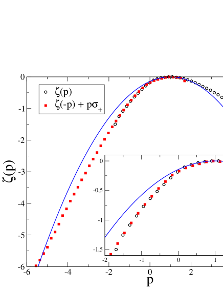
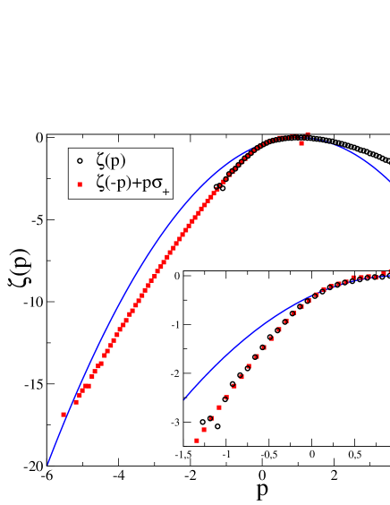
Figure 2: Two examples of the function $\zeta_{\infty}(p)$ measured in a numerical simulation [49]. Open circles: $\zeta_{\infty}(p)$. Filled squares: $\zeta_{\infty}(-p)+p\sigma_{+}$. There are no free parameters. A Gaussian fit close to $p=1$ is reported as a full line. Deviations from the Gaussian are seen close to $p=0$. In the inset an enlargment of the region where circles and square overlap, allowing for a test of the fluctuation relation, is reported. It was checked [49] that in this interval of $p$ the function $\zeta_{\tau}(p)$ did not depend on $\tau$, so that it is equal to the true limiting function $\zeta_{\infty}(p)$. (Left) $N=8$ Lennard-Jones particles in $d=2$ subject to a constant force (electric field) with periodic boundary conditions and with a reversible Gaussian thermostat. (Right) Similar system with $N=20$ and $d=3$. See [49] for details on the simulation.

This problem is specific of systems which admit a natural equilibrium state and are driven far from equilibrium by some perturbation, such as a Lennard-Jones fluid. There are however systems (e.g. the Navier-Stokes equations) such that one cannot reach an equilibrium state by tuning some parameter. For these system there is no obvious linear response theory, and a test of the fluctuation relation is stringent even if the distribution is found to be Gaussian. In the case of a reversible version of the Navier-Stokes equations (to which the chaotic hypothesis can be applied), successful numerical tests of the fluctuation relation were performed in [56, 57, 58].

The numerical results cited above strongly support the claim that the chaotic hypothesis can be applied to systems verifying the requirements of section 1.6. Moreover a new very efficient method to sample large deviations has been proposed in [59] and applied to test the fluctuation relation in some systems belonging to this class, with very promising results.

3 The effect of singularities: non-smooth systems

Despite these successes, a number of simulations performed using different ensembles found apparent violations of the fluctuation relation, see e.g. [60] and references therein. These violations where later recognized to be due to the presence of singularities of the Lennard-Jones potential used in the simulation, that were affecting the measurements in a subtle way [61, 62, 63]. In a system of particles interacting through a Lennard-Jones potential, the potential energy can be arbitrarily large if two particles are close enough to each other. If energy is conserved, this cannot happen, but it can happen, for instance, if only the kinetic energy is kept constant. This is why violations were observed only when using the isokinetic thermostat.

Consider the power injected into the system by the external forcing, $W(t)$, and the heat per unit time, $Q(t)$, dissipated by the thermostat. Energy conservation implies $Q(t)=W(t)-\dot{E}(t)$, where $E=K+V$ is the total energy. Thus if the latter is conserved, $Q=W$, while if kinetic energy is constant, $Q(t)=W(t)-\dot{V}(t)$, where $V(t)$ is the potential energy in the system. The entropy production rate, $\sigma(t)$, can be defined as $\sigma_{W}(t)=W(t)/T$ or as $\sigma_{Q}(t)=Q(t)/T$; there is no a priori reason for choosing one of the two definitions. The difference is a total derivative that has zero average in stationary state, so the average $\sigma_{+}$ is unaffected by the choice.

If one considers a microscopic model of the system, it turns out that the phase space contraction rate, as computed from the equations of motion, can be given by any of the two definitions above, depending on which metric one uses to measure distances in phase space. In fact, the phase space contraction rate is defined with respect to a given metric $\mu(x)dx$ and if one switches from $\mu(x)$ to $\mu(x)e^{-\varphi(x)}$ the phase space contraction rate is changed by $\dot{\varphi}$, see Appendix A. For instance, in the case discussed above, the phase space contraction rate is given by $W(t)/T$ if one considers the contraction of the measure $\mu(p,q)dpdq=e^{-\beta V(q)}\delta(K(p)-3NT/2)dpdq$, $(p,q)$ being the momenta and positions of the particles, and by $Q(t)/T$ if one considers the contraction of the volume measure $dpdq$.

What is the effect of the total derivative $\dot{V}$? If we consider the integrated variables,

$$\sigma_{Q\tau}=\frac{1}{\tau}\int_{0}^{\tau}\frac{Q(t)}{T}=\sigma_{W\tau}+\frac{V(0)-V(\tau)}{\tau T}\ .$$ (28)

If $V(q)$ is a bounded function, $|V(q)|\leq B$, the difference vanishes as $1/\tau$ for large $\tau$. This happens uniformly on phase space and it follows that the large deviation functions of $\sigma_{W}$ and $\sigma_{Q}$ are equal. Thus, for what concerns asymptotic statements such as the fluctuation relation, the two definitions are equivalent. The fluctuation relation does not depend on the measure one chooses to compute the phase space contraction rate, as anticipated in section 1, as long as $\sigma$ is smooth and bounded.

3.1 The effect of an unbounded total derivative

Let us now see what happens if the function $V$ is not bounded. The effect of an unbounded total derivative term was first discussed in [61] and [64, 62]. Extensions were discussed in [63, 65, 36, 66]. Here we will follow and extend the derivation in [63]. As part of the computation is unpublished, all the details are given in Appendix D.

We consider the normalized variables $p_{Q}=\sigma_{Q\tau}/\sigma_{+}$ and $p_{W}=\sigma_{W\tau}/\sigma_{+}$, verifying the relation

$$p_{Q}=p_{W}+\frac{v_{i}-v_{f}}{\tau}\ ,$$ (29)

having defined the function $v(t)=V(t)/(T\sigma_{+})$. The potential energy is usually bounded from below, $V(t)\geq B$. As only differences of $V$ matter, we assume that $B=0$ by a shift of $V$, without loss of generality. We assume that $p_{W}$ has a well defined large deviation function,

$$P_{\tau}(p_{W})\sim e^{\tau\zeta_{W}(p_{W})}\ ,$$ (30)

and we define

$$P(v)=e^{-f(v)}\ ,$$ (31)

the probability distribution of both $v_{i}$, $v_{f}\geq 0$.

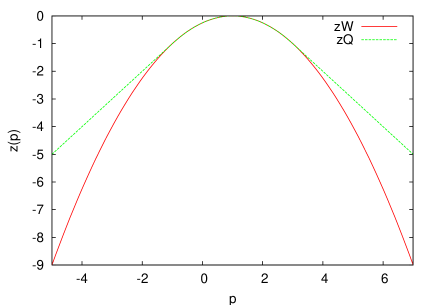
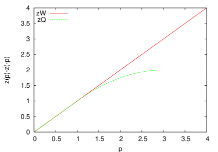
Figure 3: The case of exponential tails. In this case $\zeta_{W}(p)=-\frac{(p-1)^{2}}{4}$ verifies the fluctuation relation for $\sigma_{+}=1$, and $A=1$, hence $P(v)=e^{-v}$. The corresponding function $\zeta_{Q}(p)$ coincides with $\zeta_{W}(p)$ only for $p\in[-1,3]$, and does not verify the fluctuation relation for $p>1$ [62, 7].

We assume that $p_{W}$, $v_{i}$ and $v_{f}$ are independent; this follows from the chaotic hypothesis [63], because for large $\tau$, $v_{i}\propto V(0)$ and $v_{f}\propto V(\tau)$ must be uncorrelated, and $p_{W}$ is an integral of a function evaluated for $t\in[0,\tau]$ which is independent of $V(0),V(\tau)$ for most times $t$. We have then

$$\begin{split}P_{\tau}(p_{Q})&=\int_{-\infty}^{\infty}dp_{W}\int_{0}^{\infty}dv_{i}dv_{f}e^{\tau\zeta_{W}(p_{W})-f(v_{i})-f(v_{f})}\delta\left(p_{Q}-p_{W}-\frac{v_{i}-v_{f}}{\tau}\right)=\\ &=\tau^{2}\int_{0}^{\infty}dv_{i}dv_{f}e^{\tau\zeta_{W}(p_{Q}-v_{i}+v_{f})-f(\tau v_{i})-f(\tau v_{f})}\ ,\end{split}$$ (32)

where we performed the integration over $p_{W}$ using the delta function and changed variable from $v_{i,f}$ to $v_{i,f}/\tau$. For large $\tau$ we evaluate the integral at the saddle point and we obtain

$$\zeta_{Q}(p_{Q})=\frac{1}{\tau}\log P_{\tau}(p_{Q})\sim\max_{v_{i},v_{f}}\left\{\zeta_{W}(p_{Q}-v_{i}+v_{f})-\frac{1}{\tau}[f(\tau v_{i})+f(\tau v_{f})]\right\}\ .$$ (33)

The solution of the saddle point equations, detailed in Appendix D, gives the following asymptotic behavior:

• for superexponential tails, $f(v)\sim Av^{\alpha}$, $\alpha>1$, one obtains $\zeta_{Q}(p_{Q})=\zeta_{W}(p_{Q})+O(\tau^{-1})$ for all $p_{Q}$;

• for exponential tails, $f(v)\sim Av$, we get

  $$\zeta_{Q}(p_{Q})=\begin{cases}\zeta_{W}(p_{-})+A(p_{Q}-p_{-})\hskip 30.0ptp<p_{-}\ ,\\ \zeta_{W}(p_{Q})\hskip 90.0ptp_{-}<p<p_{+}\ ,\\ \zeta_{W}(p_{+})-A(p_{Q}-p_{+})\hskip 30.0ptp>p_{+}\ ,\end{cases}$$ (34)

  where $p_{\pm}$ are defined by $\zeta_{W}^{\prime}(p_{\pm})=\mp A$, i.e. $\zeta_{Q}$ coincides with $\zeta_{W}$ for $p\in[p_{-},p_{+}]$ and outside this interval it is given by its continuation by straight lines with slope $\pm A$.

• for subexponential tails, $f(v)\sim Av^{\alpha}$, $0<\alpha<1$, the values $p_{\pm}$ are defined by $|p_{\pm}-1|=\delta\sim\tau^{-\frac{1-\alpha}{2-\alpha}}$:

  $$\delta=\frac{2-\alpha}{1-\alpha}\left[\frac{\zeta_{W}^{\prime\prime}(1)}{A\alpha(\alpha-1)}\right]^{\frac{1}{\alpha-2}}\tau^{-\frac{1-\alpha}{2-\alpha}}$$ (35)

  and

  $$\zeta_{Q}(p_{Q})=\begin{cases}\zeta_{W}(p_{Q})\hskip 70.0pt|p_{Q}-1|\leq\delta\\ -A\tau^{\alpha-1}|p_{Q}-1|^{\alpha}\hskip 20.0pt|p_{Q}-1|>\gamma\end{cases}$$ (36)

  for any finite (i.e. independent of $\tau$) $\gamma\gg\delta$. In the intermediate regime $\delta\leq|p_{Q}-1|<\gamma$ the saddle point solution has to be calculated numerically to interpolate between the two regimes. The function $\zeta_{Q}(p_{Q})$ tends to zero for any $p_{Q}\neq 1$ and coincides with $\zeta_{W}$ only in a small interval around $p_{Q}=1$, whose amplitude shrinks to $0$ for $\tau\rightarrow\infty$.

• for power-law tails, $f(v)\sim\beta\log v$, we get the same as above with

  $$\delta=|p_{\pm}-1|=2\sqrt{-\frac{\beta}{\tau\zeta^{\prime\prime}_{W}(1)}}\ .$$ (37)

  and

  $$\zeta_{Q}(p_{Q})\sim-\frac{\beta}{\tau}\log[\tau|p_{Q}-1|]$$ (38)

  for $|p_{Q}-1|>\gamma$ for any finite $\gamma$.

In brief, total derivative terms with superexponential tails are irrelevant, while exponential tails give a finite modification of $\zeta_{Q}$, and subexponential tails give $\zeta_{Q}\rightarrow 0$ for all $p_{Q}$. This makes evident that total derivatives might have a dramatic effect.

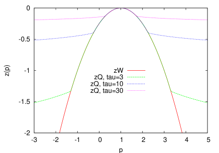
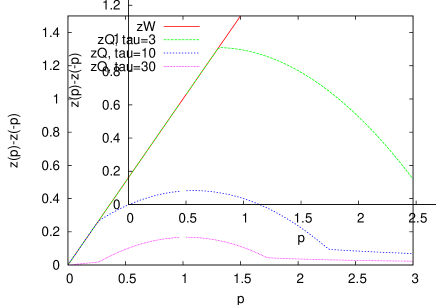
Figure 4: The case of power-law tails. $\zeta_{W}(p)$ is as in Fig. 3, while $f(v)=2\log(v)$, i.e. $P(v)\sim v^{-2}$. The function $\zeta_{Q}(p)$ is reported for $\tau=3,10,30$. In this case for $\tau\rightarrow\infty$, $\zeta_{Q}(p)\rightarrow 0$. The fluctuation relation (right panel) is verified only for small $p$ at small $\tau$. For $\tau=30$ one has $p_{-}>0$ and the fluctuation relation is never verified. Note the similarity with the curves in Fig.3 of Ref. [4].

Assume for instance that in the previous example the function $\zeta_{W}$ satisfies the fluctuation relation. If $V$ has exponential tails, from Eq. (34) it follows that the function $\zeta_{Q}$ satisfies the fluctuation relation only for $|p|<\min(p_{-},p_{+})$, while for large $p$ the function $\zeta_{Q}(p)-\zeta_{Q}(-p)\sim$ const, see Fig. 3 for an example. Even worse, in the case of subexponential or power-law tails, $\zeta_{Q}$ satisfies the fluctuation relation only for $|p|<-p_{-}$, with $p_{-}\rightarrow 1$ for $\tau\rightarrow\infty$. Thus for large enough $\tau$ the fluctuation relation is violated for all $p$, see Fig. 4, and $\zeta_{Q}(p)-\zeta_{Q}(-p)\rightarrow 0$. It is interesting to remark that if $\zeta_{W}$ is convex, $\zeta_{Q}$ is not if the tails are subexponentials.

The case of exponential tails is particularly relevant because in many cases $v\propto V(q)$, the potential energy, whose distribution has tails $e^{-\beta V}$, i.e. exponentials. Cases in which the tails are subexponentials might be also relevant for experiments: for instance the anomalous tails in [4, 5, 8] might be explained by this computation.

3.2 Removing unbounded total derivatives

The conclusion of the previous section is that terms that are apparently small may affect dramatically the large deviations of $\sigma$ in presence of singularities. Still the two definitions of entropy production rate seem a priori equivalent from a thermodynamic point of view, and have the same average $\sigma_{+}$ and the same moments $\langle\sigma^{k}\rangle$ for any finite $k$ (the moments being related to derivatives in $p=1$ of $\zeta_{\infty}(p)$).

How can we identify a priori the correct microscopic definition of $\sigma$, satisfying eventually the fluctuation relation? A possible prescription has been discussed in [63] and is based on the proof of the fluctuation relation for continuous-time systems given in [34]. The proof is based on a Poincaré’s section mapping the continuous-time flow into a discrete-time map. One considers a set of timing events: for instance, in a system of hard spheres, the times at which two particles collide, or, similarly, in Lennard-Jones systems, the times at which the total potential energy equals a suitable value $V_{0}$. In such a way the flow is reduced to a map, and the proof of the fluctuation theorem for maps [19] can be applied. However, the Poincaré’s section, i.e. the definition of timing events, has to be chosen carefully, in such a way that the resulting map is an Anosov map. This has been rigorously done for Anosov flows in [34].

For realistic systems this is clearly very difficult. Anyway, it seems very natural, if the system has singularities, to choose the timing events in such a way that singularities are avoided. For instance, if the potential energy $V(t)$ of the system can become infinite in some points of phase space, one can choose the timing events $t_{n}$ by $V(t_{n})=V_{0}$. In the example of the previous section, Eq. (28), the two definitions of $\sigma$ become equivalent on the Poincaré’s section. More generally, if singularities are avoided by the Poincaré’s section, all possible definitions of the phase space contraction rate $\sigma(t)$ differ by a bounded total derivative which gives no contribution in the limit $\tau\rightarrow\infty$.

In this way we can remove the ambiguity on the definition of $\sigma$, at least in the limit $\tau\rightarrow\infty$. Note that this prescription does not guarantee that the phase space contraction for the discrete-time system is bounded. The possible values of the latter quantity are given by

$$\sigma_{n}=\frac{1}{t_{n+1}-t_{n}}\int_{t_{n}}^{t_{n+1}}\sigma(t)dt\ ,$$ (39)

and if $\sigma(t)$ is not integrable close to a singularity $\sigma_{n}$ can be unbounded. This happens clearly if $\sigma(t)\propto(t-t_{0})^{-\gamma}$, $\gamma<1$, for a singularity $t_{0}\in[t_{n},t_{n+1}]$. In most interesting applications, e.g. driven Lennard-Jones systems in contact with a thermostat, it is possible to show that $\sigma_{W}$ is bounded on all phase space, so that the singularities come only from the total derivative and are obviously integrable as in (28). In these cases the prescription on the Poincaré’s section is enough to remove singularities, and if the system verifies the conditions 1), 3), 4) of section 1.6, i.e. it is reversible, chaotic and has a dense attractor, the fluctuation relation is expected to hold from the chaotic hypothesis.

3.3 A proposal for data analysis in presence of singular terms

To summarize, singularities might have important effects but these can be controlled, following the computation and the prescription of the previous sections.

First of all we note that the presence of unbounded terms is manifested by anomalous tails in $\zeta_{\infty}(p)$, exponentials or possibily subexponentials. It might also be manifested by the fact that $\zeta_{\infty}(p)$ is not convex. A fit to the tails of the measured $\zeta_{\infty}(p)$ allows to guess the behavior of the tails of the singular term, as the behavior of $\zeta_{\infty}(p)$ for large $p$ is the same as the behavior of $f(v)$ for large $v$.

Assume that we have performed an experiment or a numerical simulation whose output is a very long time trace $\sigma(t)$, $t\in[0,T]$, where one has chosen a definition of $\sigma(t)$ in terms of work, heat, etc. The usual procedure to verify the fluctuation relation is to fix a time delay $\tau$, and integrate $\sigma(t)$ over subsequent segments of the trajectory to obtain values of $\sigma_{\tau}=\tau^{-1}\int_{t_{0}}^{t_{0}+\tau}\sigma(t)dt$. One then constructs the histogram $P(\sigma_{\tau})$ and the function $\zeta_{\infty}(p)$ which is used to test the fluctuation relation.

In presence of singularities, the procedure must be modified as follows:

• One defines in a suitable way a set of timing events on the trajectory, $t_{n}$, such that $\sigma(t)$ is not singular for $t=t_{n}$, and that the average difference between two subsequent timing events is finite, $\tau_{0}=\langle t_{n+1}-t_{n}\rangle<\infty$.

• One fixes a delay $k$ and constructs values of

  $$\sigma_{k}=\frac{1}{t_{n+k}-t_{n}}\int_{t_{n}}^{t_{n+k}}dt\sigma(t)\ .$$ (40)

• Then one constructs the histogram $P_{k}(\sigma_{k})$ and the large deviation function $\zeta_{k}(p)=k^{-1}\log P_{k}(p\sigma_{+})$, where $\sigma_{+}=\langle\sigma_{k}\rangle$; the latter can be used to test the fluctuation relation in the limit $k\rightarrow\infty$.

If the system is reversible, chaotic and has a dense attractor, the function $\zeta_{k}(p)$ should have a finite limit that will be convex and verify the fluctuation relation (8) for large $k$, according to the chaotic hypothesis.

Then, to check the consistency of the analysis, one can recompute the original large deviation function $\zeta_{\infty}(p)$. Indeed a guess on the tails of the function $v_{i,f}$ can be done by looking at the tails of the function $\zeta_{\infty}(p)$, because as we discussed above the two functions have the same tails. Using this guess, one can apply the formulas of section 3.1 and check the self-consistency of the analysis.

The analysis of this section has been confirmed in some cases by numerical simulations [48, 49, 67], and experimentally [7], and seems promising to interpret recent experiments on turbulent systems [4, 5].

Unfortunately, if $\sigma$ is not integrable between two timing events, i.e. (39) is not bounded, at present no general statement can be made. However this seems to be a very pathological case which should not be realized in most physical examples.

4 On the convergence of the transient fluctuation relation to the stationary state fluctuation relation

As we discussed in the introduction, even if it may seem that the transient fluctuation relation implies the fluctuation relation for stationary state in the limit $\tau\rightarrow\infty$, this is not the case in general. The transient fluctuation relation holds in greater generality than the stationary state fluctuation relation. In this section we will discuss some examples that will highlight the importance of the properties of chaoticity and transitivity (i.e. the property that the attractor is dense in phase space) to ensure the validity of the fluctuation relation.

As we said in the introduction, chaoticity is important because it guarantees that initial data sampled with respect to the volume measure produce trajectories converging fast enough to the stationary state. Indeed, in experiments the system is often prepared at equilibrium, then the driving force is turned on and the system is let evolve toward the stationary state. If convergence to the stationary state is not fast enough, the observed trajectories might not be representative of the real stationary state, and confusing results may be obtained.

4.1 Examples of systems such that $P_{eq}$ does not converge to the stationary state distribution

4.1.1 A simple example

A very simple example in which the distribution $P_{eq}$ does not converge to the stationary state distribution has been given in [33]. In this example the transient fluctuation relation holds for any finite time $\tau$, including the $\tau\rightarrow\infty$ limit, for $P_{eq}$, but the real stationary state distribution trivially violates the fluctuation relation.

The model describes a free particle evolving in two dimensions under the action of a constant force $\vec{E}$ and of a thermostatting force keeping its kinetic energy constant. If $\vec{p}$ is the momentum of the particle, its mass is $1$ and we fix $|\vec{p}|^{2}=1$, the equation of motion are

$$\dot{\vec{p}}=\vec{E}-(\vec{E}\cdot\vec{p})\vec{p}\ ,$$ (41)

and introducing the angle $\theta$ by $\vec{p}\cdot\vec{E}=E\cos\theta$, where $E=|\vec{E}|$, we can write the equation for $\theta$:

$$\dot{\theta}=-E\sin\theta\ .$$ (42)

The dissipated power is given by $W(t)=\vec{E}\cdot\vec{p}(t)=E\cos\theta(t)$ and is equal to the entropy production rate, the “temperature” $|\vec{p}|^{2}$ being equal to $1$. Note that $W(t)=d\dot{\theta}/d\theta$ is the phase space contraction rate for Eq. (42).

The equation of motion (42) with initial datum $\theta_{0}$ is easily solved,

$$\tan\frac{\theta(t)}{2}=e^{-Et}\tan\frac{\theta_{0}}{2}\ .$$ (43)

The entropy production rate over the trajectory is given by, defining $s(t)=\tan\theta(t)/2$,

$$\begin{split}\sigma_{\tau}&=\frac{1}{\tau}\int_{0}^{\tau}dtE\cos\theta(t)=\frac{1}{\tau}\int_{0}^{\tau}dt\frac{\dot{\theta}E\cos\theta(t)}{-E\sin\theta(t)}=-\frac{1}{\tau}\int_{\theta_{0}}^{\theta(t)}\frac{d\theta}{\tan\theta}\\ &=-\frac{1}{\tau}\log\frac{\sin\theta(\tau)}{\sin\theta_{0}}=E-\frac{1}{\tau}\log\frac{1+s^{2}_{0}}{1+e^{-2E\tau}s^{2}_{0}}\ ,\end{split}$$ (44)

and it is easy to see that $\sigma_{\tau}\in[-E,E]$.

The distribution $P^{\theta}_{eq}(\sigma_{\tau})$ is computed imposing uniform distribution over the inital data $\theta_{0}$. Then, inverting (44) to express $s_{0}$ as a function of $\sigma_{\tau}$, we have

$$P^{\theta}_{eq}(\sigma_{\tau})=\frac{1}{2\pi}\left|\frac{d\theta_{0}}{d\sigma_{\tau}}\right|=\left|\frac{1}{4\pi s_{0}(1+s_{0}^{2})}\frac{ds_{0}}{d\sigma_{\tau}}\right|=\frac{1}{4\pi\sqrt{(e^{\tau(E-\sigma_{\tau})}-1)(1-e^{-\tau(E+\sigma_{\tau})})}}\ .$$ (45)

It is easy to check that this distribution verifies $P^{\theta}_{eq}(-\sigma_{\tau})=e^{-\tau\sigma_{\tau}}P^{\theta}_{eq}(\sigma_{\tau})$ for any finite time and that in the limit $\tau\rightarrow\infty$ we have, for $p=\sigma_{\tau}/E\in(-1,1)$,

$$\widetilde{\zeta}_{\infty}(p)=\lim_{\tau\rightarrow\infty}\frac{1}{\tau}\log P^{\theta}_{eq}(pE)=E\frac{p-1}{2}\ ,$$ (46)

such that $\widetilde{\zeta}_{\infty}(p)-\widetilde{\zeta}_{\infty}(-p)=Ep=\sigma_{+}p$, i.e. the limiting distribution verifies the fluctuation relation.

The stationary state corresponds to $\theta=0$, then $s=0$ and $\sigma_{\tau}=E$; thus the distribution

$$P^{\theta}_{st}(\sigma_{\tau})=\delta(\sigma_{\tau}-E)$$ (47)

trivially violates the fluctuation relation.

4.1.2 Another simple example

In the previous example the stationary state function $\zeta_{\infty}(p)$ does not exist because $P^{\theta}_{st}$ is singular. One might argue that this pathology is responsible for the difference between $\zeta_{\infty}$ and $\widetilde{\zeta}_{\infty}$. However this is not the case. Consider as an example a system whose state variable is an independent pair $(x,\theta)$ with $\theta$ evolving according to (42), and $x$ describing a reversible Anosov system. The phase space contraction rate is

$$\Sigma(x,\theta)=E\cos\theta+\sigma^{x}(x)\ ,$$ (48)

where $\sigma^{x}(x)$ is the contraction rate of the Anosov system. The distribution of $\Sigma_{\tau}=\tau^{-1}\int_{0}^{\tau}dt[E\cos\theta(t)+\sigma^{x}(x(t))]$ is given, if initial data are sampled according to the volume measure, by

$$P_{eq}(\Sigma_{\tau})=\int d\sigma^{x}_{\tau}P^{\theta}_{eq}(\Sigma_{\tau}-\sigma^{x}_{\tau})P^{x}_{eq}(\sigma^{x}_{\tau})\ ,$$ (49)

with $P^{\theta}_{eq}$ given by (45). Given that both $P^{\theta}_{eq}$ and $P^{x}_{eq}$ verify the transient fluctuation relation (10), it follows easily that $P_{eq}(\Sigma_{\tau})$ verifies the same relation for any finite $\tau$ and consequently the limit distribution $\widetilde{\zeta}_{\infty}(p)=\lim_{\tau\rightarrow\infty}\tau^{-1}\log P_{eq}(p\Sigma_{+})$ verifies the fluctuation relation. Conversely, the distribution in stationary state is

$$P_{st}(\Sigma_{\tau})=\int d\sigma^{x}_{\tau}P^{\theta}_{st}(\Sigma_{\tau}-\sigma^{x}_{\tau})P^{x}_{st}(\sigma^{x}_{\tau})=\int d\sigma^{x}_{\tau}\delta(\Sigma_{\tau}-\sigma^{x}_{\tau}-E)P^{x}_{st}(\sigma^{x}_{\tau})=P^{x}_{st}(\Sigma_{\tau}-E)\ ,$$ (50)

and, given that $P^{x}_{st}$ verifies the fluctuation relation, it is easy to see that the relation is not verified by $P_{st}(\Sigma_{\tau})$, neither for finite $\tau$ nor in the limit $\tau\rightarrow\infty$ (this statement can be checked for instance assuming that $P^{x}_{st}$ is a Gaussian).

To summarize, in this example the distribution $\tau^{-1}\log P_{eq}(\Sigma_{\tau})$ converges fast enough to a limiting distribution $\widetilde{\zeta}_{\infty}(p)$ verifying the fluctuation relation. The true distribution $\zeta_{\infty}(p)=\lim_{\tau\rightarrow\infty}\tau^{-1}\log P_{st}(\Sigma_{\tau})$ exists, is analytic, but is different from $\widetilde{\zeta}_{\infty}(p)$ and in particular does not verify the fluctuation relation.

This example shows that the limiting procedure involved in passing from the transient fluctuation relation to the stationary state fluctuation relation is very subtle. In this example nothing seems to go wrong, all the functions are smooth and convergence is fast, but the true stationary state distribution is different from the limit of the distribution $P_{eq}$. This kind of subtlety is peculiar to systems that do not display a chaotic behavior at least on some subset of the state variables, and might be very difficult to detect in a numerical experiment.

4.2 Hidden time scales

The strange behavior of the examples above can be related to the existence of a hidden very large time scale. This time scale can be revealed by adding a small noise term of variance $\varepsilon$ to Eq. (42). In presence of the noise, the system is able to explore the full phase space and the fluctuation relation holds in stationary state for any finite $\varepsilon$. However, in the limit $\varepsilon\rightarrow 0$, the time needed is $\tau_{\varepsilon}\sim e^{1/\varepsilon}$. For $\tau\ll\tau_{\varepsilon}$ the fluctuation relation is violated, while for $\tau\gg\tau_{\varepsilon}$ it is recovered. Clearly in the limit $\varepsilon\rightarrow 0$, $\tau_{\varepsilon}\rightarrow\infty$ and the fluctuation relation is violated for all $\tau$ in stationary state [68].

As a simple example we consider a two-state system described by a spin variable $s_{t}\in\{-1,1\}$. The initial spin is chosen from $P(s_{0})\propto e^{hs_{0}}$, then the transition rate $K(s_{t},s_{t+1})$ is proportional to $e^{hs_{t+1}-\beta J(s_{t},s_{t+1})}$, where $J(+,-)=1$ and $J=0$ otherwise, i.e. $J(s,t)=\delta_{s,+}\delta_{t,-}$. Then the probability of a trajectory $s=(s_{0},\cdots,s_{\tau})$ is given by

$$P[s]\propto e^{h\sum_{t=0}^{\tau}s_{t}-\beta\sum_{t=0}^{\tau-1}J(s_{t},s_{t+1})}\ ,$$ (51)

i.e. the dynamical system corresponds to a one-dimensional Ising chain where only pairs $(+,-)$ give a contribution $1$ to the energy.

Define the time reversed trajectory $\bar{s}=(-s_{\tau},\cdots,-s_{0})$; then

$$P[\bar{s}]=e^{-2h\sum_{i=0}^{\tau}s_{i}}P[s]=e^{-\tau\sigma_{\tau}[s]}P[s]\ ,$$ (52)

and this implies the fluctuation relation for the distribution of

$$\sigma_{\tau}[s]=\frac{2h}{\tau}\sum_{t=0}^{\tau}s_{t}\ ,$$ (53)

for any finite $\beta$.

For infinite $\beta$ the transition $(+,-)$ is forbidden: therefore, in stationary state only the trajectory $s=(+,+,\cdots,+)$ is possible. Thus $P_{st}(\sigma_{\tau})=\delta(\sigma_{\tau}-2h)$ and it does not verify the fluctuation relation, as in the examples discussed above. Note that transient trajectories of the form $(-,\cdots,-,+,\cdots,+)$ are allowed, if initial data are extracted according to $P(s_{0})\propto e^{hs_{0}}$, and the relation (52) holds for these transient trajectories. Then the transient fluctuation relation holds for $P_{eq}$ also for $\beta=\infty$ at any finite $\tau$, and in the limit $\tau\rightarrow\infty$. This is exactly the same situation we already discussed in section 4.1.1.

The limit of very large but finite $\beta$ is particularly interesting: in this limit, the Ising chain (51) develops a large correlation length. Consider a segment of trajectory of length $\ell$ beginning with $+$. The segment $(+,\cdots,+)$ has probability $O(1)$. Segments ending in the state $-$ have at least one interface $(+,-)$ which can be everywhere in $\ell$, then their probability is $\sim\ell e^{-\beta}$. Therefore if one wants to observe a jump $(+,-)$ the segment of trajectory must have length $\ell\sim e^{\beta}$. This is the time we need to wait if we want to observe a jump to the state $-$ which is needed to observe the fluctuation relation. We conclude that if $\tau\ll e^{\beta}$ the fluctuation relation will be violated, while if $\tau\gg e^{\beta}$ it will be verified.

In the limit $\beta\rightarrow\infty$, the time scale diverges and this is why the fluctuation relation is violated also in the limit $\tau\rightarrow\infty$: the limits $\beta\rightarrow\infty$ and $\tau\rightarrow\infty$ cannot be exchanged [68].

4.3 Transitive Axiom C attractors

The system (48) is a particular case of a more generic situation in which the motion of the system on its attractor can be described by a transitive Anosov system. If the system is reversible, and there is a unique attractor ${\cal A}_{+}$ and a unique repeller ${\cal A}_{-}$ (i.e. an attractor for the time-reversed dynamics), the system is called an Axiom C system. Details can be found in [45, 44].

An extended version of the chaotic hypothesis is that, if the attracting set is not dense in phase space, the system can be regarded as an Axiom C system, i.e. the motion on the attracting set is described by an Anosov system, at least for the purpose of computing the physically interesting quantities. The SRB measure describing the stationary state will be given by an expression similar to (3), with the expansion rates computed on the attractor, times a “delta function” enforcing the constraint that the system is on the attractor.

In such systems, the phase space contraction rate can be written as in (48):

$$\Sigma(x)=\sigma_{\cal A}(x)+\sigma_{\perp}(x)\ ,$$ (54)

where $\sigma_{\cal A}(x)$ describes the phase space contraction rate on the attractor, while $\sigma_{\perp}(x)$ describes the part which is orthogonal to the attractor. One could then be interested in measuring the fluctuation of $\sigma_{\cal A}(x)$ to test the extended chaotic hypothesis, that implies that $P(\sigma_{\cal A})$ verifies the fluctuation relation. Unfortunately, in general the attractor will be a complicated manifold and the explicit construction of $\sigma_{\cal A}(x)$ might be impossible. In particular, while $\Sigma(x)$ is related to the entropy production rate, it is not obvious to relate $\sigma_{\cal A}(x)$ to an experimentally accessible quantity.

A possible strategy to access $\sigma_{\cal A}(x)$, that works under some additional hypothesis, has been proposed in [45, 44]. Unfortunately for the moment a numerical verification of this proposal is not possible due to prohibitive computational costs [49], so we will not discuss this matter in more detail here.

4.4 Summary

We discussed some examples in which the transient fluctuation relation holds but the stationary state fluctuation relation is violated. This is due to the fact that (a subset of the) system is not chaotic, and might be related to a diverging “hidden” time scale whose existence can be revealed by adding a small noise [68].

5 Irreversible systems

In the previous section we discussed some possible violation and/or modification of the fluctuation relation for systems that violate the requirements of smoothness, chaoticity and ergodicity/transitivity. The last ingredient which is required, as discussed in section 1.6, is the requirement of reversibility. This requirement is crucial: indeed, we see from Eq. (6) that the fluctuation relation compares the probability of trajectories ${\bf x}(t)$ having positive entropy production rate with the probability of their time reversed $I{\bf x}(t)$ having negative entropy production rate. If the system is not reversible, nothing guarantees that the latter exist: the entropy production could be always positive and obviously Eq. (6) does not make sense in this case.

5.1 Reversible and irreversible models

We will now discuss some examples [45, 69, 70] in which one can construct two models, one reversible and the other irreversible, that seems to describe the same physical system. We will see that the result for the large deviation function of the global entropy production rate, $\zeta_{\infty}(p)$, is very different. We will then discuss in what sense the two models might be equivalent.

5.1.1 Reversible Gaussian thermostat and constant friction thermostat

A class of reversible models which is believed to describe nonequilibrium systems are based on Gaussian thermostats. Consider a system of particles described by their position and momenta $(p_{i},q_{i})$ with equations of motion

$$\begin{split}m\dot{q}_{i}&=p_{i}\ ,\\ \dot{p}_{i}&=-\partial_{q_{i}}V(q)+F_{i}(q)-\alpha(p,q)p_{i}\ .\\ \end{split}$$ (55)

Here $V(q)$ is the potential energy of interaction between particles, and $F(q)$ represents an external driving force that does not derive from a potential and injects energy into the system. The Gaussian multiplier $\alpha(p,q)$ is defined by the condition that the total energy $H(p,q)=\sum_{i}\frac{p^{2}_{i}}{2m}+V(q)$, or the kinetic temperature $T(p)=\frac{1}{Nd}\sum_{i}\frac{p^{2}_{i}}{m}$, are constant. In the former case one has

$$\alpha(p,q)=\frac{\sum_{i}p_{i}F_{i}(q)}{\sum_{i}p_{i}^{2}}\ .$$ (56)

Models belonging to this class are often used to model electric conduction, shear flow, heat flow, and so on, see e.g. [51] for a review. The equations (55) are reversible, the time reversal being simply $I(p(t),q(t))=(-p(-t),q(-t))$.

The phase space contraction rate for this equation is easily computed and gives

$$\sigma(p,q)=\sum_{i}\frac{d\dot{p}_{i}}{dp_{i}}+\frac{d\dot{q}_{i}}{dq_{i}}=Nd\alpha(p,q)+O(N^{-1})=\frac{\sum_{i}\dot{q}_{i}F_{i}(q)}{(Nd)^{-1}\sum_{i}p_{i}^{2}/m}=\frac{W(p,q)}{T(q)}\ ,$$ (57)

where $W(p,q)$ is the power injected by the external force. This result is an example of the identification between phase space contraction rate and entropy production rate we already discussed.

The Gaussian multiplier $\alpha(p,q)$ is a quantity $O(1)$ in the thermodynamic limit, and we expect its fluctuations to be $O(1/\sqrt{N})$. Therefore, in the thermodynamic limit, we can replace $\alpha(p,q)$ by its average $\nu=\langle\alpha(p,q)\rangle$, in the equation of motion (55):

$$\begin{split}m\dot{q}_{i}&=p_{i}\ ,\\ \dot{p}_{i}&=-\partial_{q_{i}}V(q)+F_{i}(q)-\nu p_{i}\ .\\ \end{split}$$ (58)

But if we do this, the new equations are not reversible! Moreover, the phase space contraction rate is now $\sigma_{\nu}(p,q)=Nd\nu$ and is always positive, so certainly the fluctuation relation does not hold for this quantity. We can ask whether the phase space contraction rate of the reversible equations, given by (57) and identified with the entropy production rate, still verifies the fluctuation relation if studied using the irreversible equations of motion (58). This is not the case. We have, from the definition of $H$,

$$\frac{dH}{dt}=\sum_{i}\dot{q}_{i}F_{i}(q)-\nu\sum_{i}\frac{p_{i}^{2}}{m}\ .$$ (59)

Using this relation, Eq. (57) becomes

$$\sigma(p,q)=Nd\nu+\frac{1}{T(p)}\frac{dH}{dt}\ .$$ (60)

The first term is always positive. For large $N$, the second term averaged over a time $\tau$ is roughly equal to $\frac{1}{\tau}\frac{\Delta H}{\left\langle T(p)\right\rangle}$ and will vanish for $\tau\rightarrow\infty$ if $H$ is bounded. Therefore the integral of $\sigma(p,q)$ in (57) is always positive for large $\tau$, and the fluctuation relation cannot hold for this quantity.

We conclude that the large deviations of $\sigma(p,q)$ are different in the two cases, and in the irreversible case do not verify the fluctuation relation.

This is not surprising, since $\sigma(p,q)$ is a global quantity, and it is well known in equilibrium statistical mechanics that global quantities can have very different behavior if computed in different ensembles.

Instead, the two equations (55) and (58) might be equivalent for the purpose of computing properties of local observables, i.e. quatities that depend only on the particles which are in a small box inside the system, in the thermodynamic limit. In this case the equivalence might hold also for large deviations. We will discuss this point in the following sections.

5.1.2 Turbulence and the Navier-Stokes equations

Another interesting example is the case of the Navier-Stokes equations. These equations are not reversible. However, it has been conjectured in [69, 23] that the Navier-Stokes equations might be equivalent, in some situations, to reversible equations. The equivalence is in the same spirit discussed in the previous section.

Numerical results supporting this conjecture have been given in [56, 57, 58], where the validity of the fluctuation relation has been numerically verified for the reversible equations.

Note that, an argument similar to the one discussed in the previous section [70] leads to the same conclusion, that the fluctuation relation cannot hold for the global entropy production in irreversible Navier-Stokes equations.

5.1.3 The granular gas

The case of granular gases is particularly illustrative. A granular gas is a system of macroscopic particles (typically of radius $R\sim 1$ mm and mass $m\sim 1$ mg) in a container of side $L$ interacting via inelastic collisions (typically with restitution coefficient $r\sim 0.8\div 0.9$) and having a large kinetic energy $\frac{1}{2}m\langle v^{2}\rangle\gg mgR$, where $g$ is the acceleration due to gravity. Energy is injected into the system by shaking the box or vibrating one of its sides. This system behaves like a gas of hard particles but dissipation is present due to the inelasticity of the collisions.

The first experiment on such a system [8] considered a window of smaller side $\ell$ inside the box and measured the flux $P_{\tau}$ of kinetic energy entering the window during a time lapse $\tau$. The latter seemed to verify a fluctuation relation at least for small $p=P_{\tau}/\langle P_{\tau}\rangle$. Note that the kinetic energy flux can be written as

$$P_{\tau}=\Delta E+D_{\tau}\ ,$$ (61)

where $\Delta E=E(\tau)-E(0)$ is the variation of kinetic energy inside the window, while $D_{\tau}$ is the energy dissipated into the window by inelastic collisions during time $\tau$.

A very reasonable model for the inelastic collisions between particles [72, 73, 65, 70] is to assume that the velocity component parallel to the collision axis is rescaled by $r$, in such a way that the relative variation of kinetic energy in the collision is $1-r^{2}>0$. In such a model, the dissipation $D_{\tau}$ is always positive, and phase space always contracts so that $\sigma\geq 0$. It was then recognized [72] that, as $D_{\tau}\geq 0$ in this model, the fluctuation relation cannot hold for $P_{\tau}$. Indeed, if $\Delta E$ were bounded, the large deviation functions of $P_{\tau}$ and $D_{\tau}$ would coincide implying that the probability of observing a negative fluctuation of $P_{\tau}$ is zero for large $\tau$. However, $\Delta E$ is not bounded, and its probability distribution has an exponential tail, see the discussion in [65]; the method described in section 3 can be applied and shows that even if $D_{\tau}\geq 0$, $P_{\tau}$ can have negative fluctuations. This explains why such fluctuations were observed in [8]. The apparent validity of the fluctuation relation observed in [8] is probably explained by the smallness of the interval of $p$ that was accessible to the experiment, in such a way that the function $\zeta_{\infty}(p)-\zeta_{\infty}(-p)$ appeared as linear in $p$.

The conclusion is that the fluctuation relation does not hold for the quantities $D_{\tau}$ (obviously) and $P_{\tau}$ (by (61) and the results of section 3), at least if the model for inelastic collisions used in [72, 73, 65] is accepted.

One can easily construct a model of reversible inelastic collisions, in which in a collision particles can gain or loose energy, such that on average energy is lost but the dynamics is reversible. Such a model should give similar results for average quantities but will give a different result for the large deviations of $P$ and $D$, which will now probabily verify the fluctuation relation.

5.2 The time scale for reversibility

Different models, reversible or irreversible, give different results when one computes large deviations of global quantities, and in particular the fluctuation relation holds for the reversible models but does not hold for the irreversible ones.

If we want to investigate the fluctuations of the global entropy production rate, we have to ask, given a physical system on which we are performing a measurement, what is the more appropriate mathematical model, between the reversible and the irreversible ones, to describe its properties?

Let us discuss this problem for the granular gas we modeled above. It is reasonable that the real system is described, at an atomic level, by reversible equations of motion (i.e. the Newton equations for the atoms constituting the macroscopic particles). In a collisions, the atoms interact in such a way that kinetic energy of the particles is dissipated by heating the two particles. Morover sound waves can be emitted as the experiment is performed in air. Thus, in principle, it can happen that two particles, while colliding, absorb a sound wave and/or cool spontaneously in such a way that the kinetic energy is augmented by the collision. Clearly, the probability of such a process is very small: it is of the order of $\exp(-N)$, where $N\sim 10^{23}$ is the number of atoms constituting a particle. Thus, on the experimental time scale $\tau\ll\tau_{0}\exp(N)$ one can safely neglect this possibility, the system is well described by the model in which velocity are rescaled by $r$ at each collision, and the fluctuation relation does not hold. However, if one could imagine to wait for a time $\tau\gg\tau_{0}\exp(N)$, the fluctuation relation should be observed to hold. In this case the violation of the fluctuation relation is related to a mechanism very similar to the one discussed in section 4.2, i.e. it is related to an “hidden” diverging time scale (the time scale on which reversibility of the collisions can be observed).

When the time scale needed for observe reversibility is not larger that the experimentally accessible time scales, the system should be well described by reversible models.

5.2.1 A proposal for an experiment on granular gases

An example of this procedure was discussed in [74]. We considered a two dimensional granular gas contained in a box; the bottom of the box is vibrated while the other sides are fixed. This geometry is different from the one considered in [8] where the whole box is vibrated.

In this situation, a temperature profile is established in the system; kinetic energy is injected at the bottom and starts to flow trough the system towards the top of the box, being dissipated in the meanwhile by inelastic collisions. The energy dissipated by collisions is again always positive, and obviously cannot satisfy the fluctuation relation.

However, one can look to a different quantity, namely the flow $J_{\tau}$ of energy through a small portion of the system located between two lines at height $h$, $h+\delta$. This quantity is not always positive and cannot be expressed as a positive quantity plus a total derivative, as we did for $P_{\tau}$ in (61). We argued that, in a suitable quasi-elastic limit [74], see also [75], the portion of the system between $h$, $h+\delta$ can be thought as being equivalent to a system of elastic hard particles in contact with two thermostats at different temperatures $T_{+}$, $T_{-}$. This system can be described by a reversible model [74]. This analysis predicts that the fluctuation relation should hold for $J_{\tau}$ at least in a suitable quasi-elastic limit. It should be possible to verify experimentally (or at least numerically) this prediction.

5.3 Ensemble equivalence

As we discussed in the previous section, if one looks at global quantities (e.g. in a numerical simulation), the result might depend on the details of the model which is assumed to describe well the system under investigation. In particular, the choice between a reversible and an irreversible model should be motivated by a careful analysis of the involved time scales.

However, this is not so natural. In fact, one of the main results of equilibrium statistical mechanics is that the relation between the interesting observables (pressure, density, energy, …) are independent of the particular ensemble one chooses to describe the system. And indeed, in a real experiment, it is very difficult to distinguish between the system under investigation and the surrounding environment, and to make a detailed model of the interaction between them. For instance, one would clearly like that the result does not depend on the details of the particular device one uses to remove heat from the system, and so on.

To avoid such difficulties, one should consider the system under investigation as a subsystem of a larger system, including the thermostats, and show that the relations between the interesting observables of the subsystem do not depend on the details of the model one chooses to describe the whole system. This would also justify the use of phenomenological models like (55), (58), which are clearly unphysical as one assumes that there is a “viscous” term acting on each atom of the fluid.

Proving equivalence of ensembles in nonequilibrium is much more difficult than in equilibrium, because in the former case dynamics is important in defining the ensembles: as the SRB measure (3) explicitely depends on the dynamics of the system. For this reason no exact results are available, but only conjectures [76, 22, 23] and arguments supporting them [71, 77], see in particular [77] for a detailed discussion.

The equivalence between two different nonequilibrium ensembles can be defined as follows. We consider as an example the two models (55), (58); the equations of motion depend on a number of parameters, such as the density of particles, the interaction potential $V(q)$, the external forcing $F(q)$ etc.; having fixed these parameters, the model (55) depends on the value of the energy $E=H(p,q)$, while (58) depends on the value of $\nu$. The corresponding ensembles ${\cal E}_{E}$, ${\cal E}_{\nu}$ are the collection of the SRB distributions that describe the stationary states of (55), (58) at different $E$ or $\nu$, respectively.

Consider now a volume $V_{0}$ inside the container $V$ in which the model is defined, and a set ${\cal O}(V_{0})$ of observables $O_{V_{0}}(p,q)$ that depend only on the positions and momenta of the particles inside $V_{0}$.

The equivalence of ${\cal E}_{E}$, ${\cal E}_{\nu}$ means that in the limit $N,V\rightarrow\infty$ at fixed $N/V$ it is possible to establish a one-to-one correspondence between elements of ${\cal E}_{E}$ and ${\cal E}_{\nu}$ such that the averages of all observables $O\in{\cal O}(V_{0})$ are equal in corresponding elements.

In this example, the element $\mu_{\nu}\in{\cal E}_{\nu}$ corresponding to the element $\mu_{E}\in{\cal E}_{E}$ is defined by the condition that

$$\nu(E)=\left\langle\alpha(p,q)\right\rangle_{E}=\int dpdq\,\mu_{E}(p,q)\alpha(p,q)\ ,$$ (62)

and conversely the element $\mu_{E}$ corresponding to a given $\mu_{\nu}$ is defined by

$$E(\nu)=\left\langle H(p,q)\right\rangle_{\nu}=\int dpdq\,\mu_{\nu}(p,q)H(p,q)\ .$$ (63)

Equivalence of the two ensembles means that for all local observables $O_{V_{0}}\in{\cal O}(V_{0})$ it holds

$$\lim_{N,V\rightarrow\infty\,,\,\rho=N/V}\left\langle O_{V_{0}}(p,q)\right\rangle_{\nu(E)}=\lim_{N,V\rightarrow\infty\,,\,\rho=N/V}\left\langle O_{V_{0}}(p,q)\right\rangle_{E}\ .$$ (64)

In the case of the two ensembles defined by (55), (58), the equivalence is supported by the concentration argument discussed above, namely that for $N,V\rightarrow\infty$ the fluctuations of $\alpha(p,q)$ in the isoenergetic ensemble vanish, see [71, 77] for more detailed discussions.

5.3.1 A local fluctuation theorem

Given the definitions above, it is natural to try to define a local entropy production rate and prove for this quantity a local fluctuation theorem. In the example (55), (58), a possible definition is a local version of (57):

$$\sigma_{V_{0}}(p,q)=\frac{\sum_{i:q_{i}\in V_{0}}\dot{q}_{i}F_{i}(q)}{(Nd)^{-1}\sum_{i:q_{i}\in V_{0}}p_{i}^{2}/m}=\frac{W_{V_{0}}(p,q)}{T_{V_{0}}(q)}\ .$$ (65)

Then, the equivalence conjecture (64), applied to the average of $O_{V_{0}}(p,q)=e^{\lambda\sigma_{V_{0}}(p,q)}$ (that generates the probability distribution of $\sigma_{V_{0}}$), implies that the large deviations function $\zeta_{V_{0}}(p)$ is the same in the two ensembles, in the thermodynamic limit. In principle this function can satisfy the fluctuation relation (8) even if one of the two ensembles is irreversible. This would be a very interesting result. Unfortunately, from the theoretical point of view the problem is very difficult. A tentative theory has been discussed in [78] and a numerical verification on a simple model of coupled maps has been reported in [79].

In numerical simulations of more realistic models, see e.g. [54], the results are much more difficult to interpret. As we discussed in section 2, even in the case of a “perfect” system (i.e. smooth, reversible, and transitive) the verification of the fluctuation relation is very difficult as long as the number of particles is bigger than $\sim 20$. Taking the limit of $N\rightarrow\infty$ means that one should look at a subsystem of $\sim 10$ particles in an environment of, say, $\sim 1000$ particles, and this, at present, has prohibitive computational costs. Moreover if the volume $V_{0}$ is too small, as required by numerical simulations, one has to take into account nontrivial terms in the entropy production rate, related to the fluxes (of particles, energy, entropy) across the surface of $V_{0}$, see [74] for a tentative discussion of this problem.

On the other hand, looking at local quantities is very natural in experiments, see e.g. [2, 3, 5, 8]. However the interpretation of these experiments is not clear for the moment (see [77] for a tentative interpretation of [2]), especially because the relation between the measured quantities and the local entropy production is not straightforward. The presence of large tails in the measured distributions suggests also that unbounded terms are affecting the measurements; it would be very interesting to try to apply the analysis described at the end of section 3 to these data.

5.4 Summary

The fluctuation relation cannot hold, even locally, if the time scale to observe reversibility exceeds the experimentally accessible time scale. Nevertheless, there are system that might be well described by reversible equations of motion, if this time scale is not too large. In these cases the fluctuation relation should hold. Clarifying this issue is clearly of fundamental importance to interpret experiments on real nonequilibrium systems.

It is worth to note that even if the fluctuation relation does not hold due to irreversibility, this does not mean that the chaotic hypothesis does not apply. If the system is chaotic and smooth enough, still the stationary state should be described by the SRB measure (3). It would be very interesting to derive from the chaotic hypothesis, using the measure (3), other relations, independent of reversibility, that could be tested in experiments.

6 Conclusions

To conclude, we will briefly summarize the main points discussed in this paper.

1. The chaotic hypothesis states that the fluctuation relation will be generically verified by models that are reversible, smooth, chaotic and transitive.

2. For such models, numerical simulations have confirmed the validity of these predictions.

3. A test of the fluctuation relation, even in models verifying the hypotheses above, is made difficult by the necessity of observing negative values of $p$. In particular, one should check that the function $\zeta_{\tau}(p)=\frac{1}{\tau}\log P(p\sigma_{+})$ is independent of $\tau$ for $p\in P$. The interval $P$ must contain the origin.

4. Negative fluctuations can be enhanced by reducing the system size $N$, the observation time $\tau$, or the strength of the applied field. The observation time $\tau$ cannot be reduced arbitrarily because the fluctuation relation holds only for $\tau\gg\tau_{0}$, $\tau_{0}$ being the characteristic decorrelation time of the system. Eventually we can eliminate some finite $\tau$ corrections, e.g. by shifting $p$ in such a way that the maximum of $\zeta_{\tau}(p)$ is assumed in $p=1$.

5. If the applied field is so small that the system is close to equilibrium, and if the distribution turns out to be Gaussian over the whole accessible interval in $p$, we are not verifying the fluctuation relation, because in this case it is equivalent to the Green-Kubo relations.

6. It is important to check not only that $\zeta_{\infty}(p)-\zeta_{\infty}(-p)\propto p$, but also that the proportionality constant is $\sigma_{+}$. The linearity in $p$ could simply be due to the smallness of the accessible interval $P$.

7. The presence of singular terms in $\sigma$ (non-smooth systems) can change dramatically the behavior of $\zeta(p)$. These terms manifest in anomalous large tails; in these cases the function $\zeta(p)$ might not be convex. If these terms are present, one should remove them by applying the procedure discussed in section 3.

8. For systems that are not chaotic or not transitive any kind of strange behavior can (and has) been observed. For this reason a test of the fluctuation relation is interesting: it supports the validity of the chaotic hypothesis, i.e. that the system is chaotic and transitive (but obviously does not prove these properties).

9. If one looks to the global entropy production rate, the fluctuation relation will not hold for irreversible systems.

10. However, it is possible that different models which are globally reversible or irreversible, might be equivalent when observed on a local scale. If this is the case, a local fluctuation relation might hold independently of the model (reversible or irreversible) one chooses to describe the system on large scale.

11. This is very important for the interpretation of experiments. If the results were found to depend strongly on the details of the model, one would have to take into account all the details of the system, including the thermostat, etc.

Hopefully new experiments will be able to clarify the many open problems, in particular the last point.

Appendix A Lyapunov exponents and the phase space contraction rate

We considered a system described by the equation of motion $\dot{x}=F(x)$ where $x=(x_{1},\cdots,x_{N})$. Consider a segment of trajectory ${\bf x}(t)$, $t\in[0,\tau]$ (time can be continuous or discrete). The Jacobian matrix of the trasformation $dx(0)\rightarrow dx(\tau)$ is given by

$$\partial S_{ij}[{\bf x}(t)]=\frac{\partial x_{i}(\tau)}{\partial x_{j}(0)}\ ,$$ (66)

has eigenvalues $s_{i}[{\bf x}(t)]$, $i=1,\cdots,N$. The Lyapunov exponents can be defined as

$$\lambda_{i}[{\bf x}(t)]=\frac{1}{\tau}\log|s_{i}[{\bf x}(t)]|\ .$$ (67)

Thus positive Lyapunov exponents correspond to expanding directions, while negative exponents correspond to contracting directions.

The expansion factor is

$$\Lambda_{u}[{\bf x}(t)]=e^{\tau\sum_{i,+}\lambda_{i}[{\bf x}(t)]}=|\det\partial S_{ij}[{\bf x}(t)]_{u}|\ ,$$ (68)

where the sum $\sum_{i,+}$ is restricted only to positive exponents and the determinant is restricted to the unstable directions (corresponding to the positive exponents). The contraction factor is

$$\Lambda_{s}[{\bf x}(t)]=e^{\tau\sum_{i,-}\lambda_{i}[{\bf x}(t)]}=|\det\partial S_{ij}[{\bf x}(t)]_{s}|\ ,$$ (69)

so that the total phase space contraction rate is

$$e^{-\tau\sigma[{\bf x}(t)]}=e^{\tau\sum_{i}\lambda_{i}[{\bf x}(t)]}=|\det\partial S_{ij}[{\bf x}(t)]|=\Lambda_{u}[{\bf x}(t)]\Lambda_{s}[{\bf x}(t)]\ .$$ (70)

For very small times $\tau=dt$ and initial datum $x$ we have

$$\partial S_{ij}[x,dt]=\delta_{ij}+dt\frac{\partial F_{i}(x)}{\partial x_{j}}\ ,$$ (71)

so that

$$|\det\partial S_{ij}[{\bf x}(t)]|=1+dt\sum_{i}\frac{\partial F_{i}(x)}{\partial x_{i}}+O(dt^{2})\ ,$$ (72)

and (70) becomes

$$\sigma(x)=-\sum_{i}\frac{\partial F_{i}(x)}{\partial x_{i}}=-\nabla\cdot F(x)\ .$$ (73)

Then it follows

$$\sigma[{\bf x}(t)]=-\frac{1}{\tau}\int_{0}^{\tau}dt\nabla\cdot F(x(t))\ .$$ (74)

For the time reversed trajectory ${\bf x}(\tau-t)$, it is easy to see that

$$\partial S_{ij}[{\bf x}(\tau-t)]=\frac{\partial x_{i}(0)}{\partial x_{j}(\tau)}=\left[\partial S_{ij}[{\bf x}(t)]\right]^{-1}\ ,$$ (75)

and the sign of the Lyapunov exponents are exchanged, as it is needed for the derivation of (6).

Finally note that $\sigma(x)$ is defined by $\frac{d}{dt}dx=-\sigma(x)dx$. Then, if instead of $dx$ we use the measure $e^{-\varphi(x)}dx$, it is easy to see that

$$\sigma^{\prime}(x)=-\frac{1}{e^{-\varphi(x)}dx}\frac{d}{dt}e^{-\varphi(x)}dx=\sigma(x)+\dot{\varphi}\ ,$$ (76)

i.e. a change of metric changes $\sigma(x)$ by a total derivative.

Appendix B The transient fluctuation relation

Here we sketch the derivation of Eq. (10) for the microcanonical ensemble. The probability $P_{eq}\{\sigma[{\bf x}(t)]=\sigma\}$ is proportional to the volume $V_{0}$ of initial data $x_{0}$ such that the subsequent trajectory gives a total phase space contraction $\sigma[{\bf x}(t)]=\sigma$. Then, by definition of the phase space contraction rate, the volume of the set of the final points $x_{\tau}=x(\tau)$ will be $V_{\tau}=e^{\tau\sigma}V_{0}$. Each point $x(\tau)$ is the starting point of a time-reversed trajectory having phase space contraction rate $\sigma[{\bf x}(t)]=-\sigma$, so the volume $V_{\tau}$ is proportional to the probability $P_{eq}\{\sigma[{\bf x}(t)]=-\sigma\}$, and Eq. (10) follows.

Appendix C A precise definition of Anosov systems

An Anosov system is defined as follows [24]. Given a compact, smooth and boundaryless manifold $M$ (phase space), a map $S\in C^{2}(M)$ is an Anosov map if:

(1) For all $x\in M$ the tangent plane to $M$ in $x$, $T_{x}$, admits a decomposition $T_{x}=T^{s}_{x}\oplus T^{u}_{x}$, such that

(2) the planes $T^{s,u}_{x}$ vary continuously w.r.t. $x$, i.e. the vectors defining them are continuous functions of $x$;

(3) the angle between $T^{s}_{x}$ and $T^{u}_{x}$, defined as the minimum angle between a vector in $T^{s}_{x}$ and a vector in $T^{u}_{x}$, is not vanishing;

(4) defining $\partial S$ the linearization matrix of $S$ in $x$, i.e. $S(x+\epsilon v)=S(x)+\epsilon\ \partial S(x)\cdot v+O(\epsilon^{2})$, $x\in M$, $v\in T_{x}$, $\epsilon\in\hbox{\msytw R}$ small, the planes $T_{x}^{s,u}$ are conserved under $S$, i.e. if $v\in T_{x}^{s,u}$, then $\partial S(x)\cdot v\in T^{s,u}_{Sx}$;

(5) for all $x\in M$ and for all $v\in T^{s}_{x}$ one has $|\partial S(x)^{k}v|_{S^{k}x}\leq\Lambda^{-k}C|v|_{x}$, while for all $v\in T^{u}_{x}$ one has $|\partial S(x)^{-k}v|_{S^{-k}x}\leq\Lambda^{-k}C|v|_{x}$, $|\bullet|_{x}$ being the norm on $T_{x}$, for some constants $C,\Lambda>0$;

(6) there is a point $x$ which has a dense orbit in $M$.

The hypotheses above imply that it is possible to identify two families of smooth manifolds $M^{s,u}$ in $M$, such that $T^{s,u}_{x}$ are the tangent plane to $M^{s,u}$ in $x$, and such that points on $M^{s}$ tend to converge exponentially while points on $M^{u}$ tend to diverge exponentially under the action of $S$.

This means that for each $x\in M$ there is a stable manifold $M^{s}_{x}$ such that for all $y\in M^{s}_{x}$ one has $d(S^{k}x,S^{k}y)\leq\Lambda^{-k}Cd(x,y)$, and an unstable manifold $M^{u}_{x}$ such that for all $y\in M^{u}_{x}$ one has $d(S^{-k}x,S^{-k}y)\leq\Lambda^{-k}Cd(x,y)$, where $d(x,y)$ is the distance on $M$, see Fig. 1.

Appendix D Saddle point equation for the distribution $\zeta_{Q}$

This computation is reported in full detail as it has not been previously published. The saddle point equation corresponding to (33) are

$$\begin{split}-\zeta_{W}^{\prime}(p_{Q}-v_{i}+v_{f})&=f^{\prime}(\tau v_{i})\ ,\\ \zeta_{W}^{\prime}(p_{Q}-v_{i}+v_{f})&=f^{\prime}(\tau v_{f})\ .\end{split}$$ (77)

For large values of its argument, $f(v)$ must be an increasing function, then $f^{\prime}(v)>0$. We will see that the saddle point values of $v_{i}$ and $v_{f}$ are small. Then, if $p_{Q}>1$, the second equation (77) has no solution, because $\zeta_{W}^{\prime}(p_{Q})<0$; this means that $v_{f}$ will stick to the boundary of the integration region, $v_{f}=0$. Conversely, for $p_{Q}<1$, we have $v_{i}=0$. Finally, we get for $p_{Q}>1$

$$\zeta_{Q}(p_{Q})\sim\max_{v_{i}}\left\{\zeta_{W}(p_{Q}-v_{i})-\frac{1}{\tau}f(\tau v_{i})\right\}\ ,\hskip 30.0pt-\zeta_{W}^{\prime}(p_{Q}-v_{i})=f^{\prime}(\tau v_{i})\ ,$$ (78)

and for $p_{Q}>1$

$$\zeta_{Q}(p_{Q})\sim\max_{v_{f}}\left\{\zeta_{W}(p_{Q}+v_{f})-\frac{1}{\tau}f(\tau v_{f})\right\}\ ,\hskip 30.0pt\zeta_{W}^{\prime}(p_{Q}+v_{f})=f^{\prime}(\tau v_{f})\ .$$ (79)

In the following we will discuss the behavior for $p_{Q}>1$, the other case can be discussed in the same way.

Superexponential tails

First we assume that $f(v)\sim Av^{\alpha}$, $\alpha>1$, for $v\rightarrow\infty$, i.e. the probability of $v$ decays faster than exponentially. We have

$$-\zeta_{W}^{\prime}(p_{Q}-v_{i})=\alpha A(\tau v_{i})^{\alpha-1}\ .$$ (80)

Clearly $v_{i}$ must be small, and we get $v_{i}=\tau^{-1}[-\zeta_{W}^{\prime}(p_{Q})/\alpha A]^{1/(\alpha-1)}\propto\tau^{-1}$, and $\zeta_{Q}(p_{Q})=\zeta_{W}(p_{Q})+O(\tau^{-1})$ for all $p$.

Exponential tails

For $f(v)\sim Av$, we get

$$-\zeta_{W}^{\prime}(p_{Q}-v_{i})=A\ ,$$ (81)

As $v_{i}$ must be positive, and $\zeta_{W}^{\prime}(p_{Q})$ is negative and decreasing on incresing $p_{Q}$, the latter equation has a solution only if $\zeta_{W}^{\prime}(p_{Q})<-A$, otherwise $v_{i}=0$. Calling $p_{+}$ the solution of $\zeta_{W}^{\prime}(p_{+})=-A$, we get $v_{i}^{*}=p_{Q}-p_{+}$ and

$$\zeta_{Q}(p_{Q})=\begin{cases}\zeta_{W}(p_{Q})\hskip 50.0ptp<p_{+}\ ,\\ \zeta_{W}(p_{+})-A(p_{Q}-p_{+})\hskip 30.0ptp>p_{+}\ ,\end{cases}$$ (82)

i.e. $\zeta_{Q}$ coincides with $\zeta_{W}$ up to $p=p_{+}$ and then it is given by its continuation as a straight line with slope $\zeta^{\prime}_{W}(p_{+})$. A similar result is obtained for $p_{Q}<1$.

Subexponential tails

For $f(v)\sim Av^{\alpha}$, $0<\alpha<1$, the saddle point equation becomes

$$-\zeta_{W}^{\prime}(p_{Q}-v_{i})=\tau^{\alpha-1}A\alpha v_{i}^{\alpha-1}\ .$$ (83)

In addition to the previous solution $v_{i}\propto\tau^{-1}$, we can look for a solution such that $p_{Q}-v_{i}=1+\epsilon$ with $\epsilon$ small. Indeed as $\zeta_{W}^{\prime}(1)=0$ the left hand side will be small, and as $v_{i}\sim p_{Q}-1$ is finite the left hand side will also be small. We get then

$$-\zeta_{W}^{\prime}(p_{Q}-v_{i})\sim-\zeta_{W}^{\prime\prime}(1)(p_{Q}-1-v_{i})=\tau^{\alpha-1}A\alpha v_{i}^{\alpha-1}\ ,$$ (84)

and we recall that $-\zeta_{W}^{\prime\prime}(1)>0$. A graphical analysis of the previous equation reveals that it has no solution as long as $p_{Q}<p_{+}$; the value of $p_{+}$ is defined by the system

$$\begin{cases}-\zeta_{W}^{\prime\prime}(1)(p_{Q}-1-v_{i})=\tau^{\alpha-1}A\alpha v_{i}^{\alpha-1}\ ,\\ \zeta_{W}^{\prime\prime}(1)=\tau^{\alpha-1}A\alpha(\alpha-1)v_{i}^{\alpha-2}\ ,\end{cases}$$ (85)

whose solution is easily found

$$\begin{cases}p_{+}-1=v^{*}_{i}\frac{2-\alpha}{1-\alpha}\ ,\\ v^{*}_{i}=\left[\frac{\zeta_{W}^{\prime\prime}(1)}{\tau^{\alpha-1}A\alpha(\alpha-1)}\right]^{\frac{1}{\alpha-2}}\ .\end{cases}$$ (86)

From the above expression we find that $p_{+}-1\sim v_{i}^{*}\sim\tau^{-\frac{1-\alpha}{2-\alpha}}$. This is consistent with the hypotheses we made above. Note also that $\tau v_{i}^{*}$ is large consistently with the assumption that only the large tail of $f(v)$ is relevant for this calculation.

For $p_{Q}<p_{+}$ the saddle point equation has no solution, it follows that $v_{i}=0$ and $\zeta_{Q}(p_{Q})=\zeta_{W}(p_{Q})$. For $p_{Q}>p_{+}$, the equation has two solution. As discussed above, for finite $p_{Q}-1$ one solution is $v_{i}\sim\tau^{-1}$ while the other one is $v_{i}\sim p_{Q}-1-\epsilon$ for small $\epsilon>0$. The latter gives the maximum in (33) while the former is a minimum. The value of $\epsilon$ is given by

$$\epsilon=\frac{A\alpha(p_{Q}-1)^{\alpha-1}}{-\zeta_{W}^{\prime\prime}(1)\tau^{1-\alpha}}\ .$$ (87)

Substituting this value into (33) we get

$$\zeta_{Q}(p_{Q})\sim\frac{\zeta_{W}^{\prime\prime}(1)}{2}\epsilon^{2}-A\tau^{\alpha-1}(p_{Q}-1)^{\alpha}\sim-A\tau^{\alpha-1}(p_{Q}-1)^{\alpha}+O(\tau^{2(\alpha-1)})\ ,$$ (88)

i.e. $\zeta_{Q}(p_{Q})$ is dominated by the tail of $P(v)$ and one gets $\zeta_{Q}(p_{Q})\rightarrow 0$ for all $p_{Q}$.

For $p<1$, changing $v_{i}\rightarrow v_{f}$, we get

$$\begin{cases}1-p_{-}=v^{*}_{f}\frac{2-\alpha}{1-\alpha}\\ v^{*}_{f}=\left[\frac{\zeta_{W}^{\prime\prime}(1)}{\tau^{\alpha-1}A\alpha(\alpha-1)}\right]^{\frac{1}{\alpha-2}}\end{cases}$$ (89)

i.e. $1-p_{-}=p_{+}-1$ so that $p_{-}$ and $p_{+}$ are symmetrically distributed around $1$, and for $p_{Q}<p_{-}$

$$\zeta_{Q}(p_{Q})\sim-A\tau^{\alpha-1}(1-p_{Q})^{\alpha}+O(\tau^{2(\alpha-1)})\ .$$ (90)

To summarize, we obtain two values of $p$, $p_{\pm}$, defined by $|p_{\pm}-1|=\delta\sim\tau^{-\frac{1-\alpha}{2-\alpha}}$:

$$\delta=\frac{2-\alpha}{1-\alpha}\left[\frac{\zeta_{W}^{\prime\prime}(1)}{A\alpha(\alpha-1)}\right]^{\frac{1}{\alpha-2}}\tau^{-\frac{1-\alpha}{2-\alpha}}$$ (91)

such that

$$\begin{cases}\zeta_{Q}(p_{Q})=\zeta_{W}(p_{Q})\hskip 70.0pt|p_{Q}-1|\leq\delta\\ \zeta_{Q}(p_{Q})=-A\tau^{\alpha-1}|p_{Q}-1|^{\alpha}\hskip 20.0pt|p_{Q}-1|>\gamma\end{cases}$$ (92)

for any finite $\gamma\gg\delta$. In the intermediate regime $\delta\leq|p_{Q}-1|<\gamma$ the saddle point solution has to be calculated numerically to interpolate between the two regimes.

Power-law tails

If $v_{i,f}$ have power-law tails for large $v$, $P(v)\sim\frac{1}{v^{\beta}}$, we have $f(v)\sim\beta\log(v)$, and the saddle point equations is for $p_{Q}>1$

$$-\zeta^{\prime}_{W}(p_{Q}-v_{i})=\frac{\beta}{\tau v_{i}}\ ,$$ (93)

and as before we can expand the l.h.s. around $p_{Q}-v_{i}\sim 1$ as the r.h.s. is small:

$$-\zeta^{\prime\prime}_{W}(1)(p_{Q}-v_{i}-1)=\frac{\beta}{\tau v_{i}}\ .$$ (94)

A solution appears for $p_{Q}>p_{+}$ where

$$\delta\equiv p_{+}-1=2\sqrt{-\frac{\beta}{\tau\zeta^{\prime\prime}_{W}(1)}}\ .$$ (95)

Eq.(94) becomes

$$v_{i}^{2}-v_{i}(p_{Q}-1)+\frac{\delta^{2}}{4}=0$$ (96)

with solutions

$$v_{i}=\frac{(p_{Q}-1)}{2}\pm\sqrt{\frac{(p_{Q}-1)^{2}}{4}-\frac{\delta^{2}}{4}}\ .$$ (97)

As before the correct solution is the largest one,

$$v_{i}^{*}(p_{Q})=\frac{(p_{Q}-1)}{2}+\sqrt{\frac{(p_{Q}-1)^{2}}{4}-\frac{\delta^{2}}{4}}$$ (98)

and as before it behaves as

$$v^{*}_{i}(p_{Q})\sim p_{Q}-1-\frac{\delta^{2}}{4(p_{Q}-1)}=p_{Q}-1-\epsilon$$ (99)

for large $\tau$ (i.e. small $\delta$). Substituting $v^{*}_{i}(p_{Q})$ in Eq.(78) we get

$$\zeta_{Q}(p_{Q})=\zeta_{W}(p_{Q}-v^{*}_{i}(p_{Q}))-\beta\tau^{-1}\log[\tau v^{*}_{i}(p_{Q})]\sim-\frac{\beta}{\tau}\log[\tau(p_{Q}-1)]+O(\tau^{-1})$$ (100)

Note however that constant shifts of the order of $\log(\tau)/\tau$ are present due to the factor $\tau^{2}$ in front of Eq.(32) and from the Gaussian fluctuations around the saddle-point. An empirical way to find the constant is to impose the continuity of $\zeta_{Q}(p_{Q})$, i.e. $\zeta_{Q}(p_{+})=\zeta_{W}(p_{+})$. From this it follows

$$\zeta_{Q}(p_{Q})=\zeta_{W}(p_{Q}-v^{*}_{i}(p_{Q}))-\beta\tau^{-1}\log[2v^{*}_{i}(p_{Q})/\delta]-\zeta_{W}(1+\delta/2)+\zeta_{W}(1+\delta)\ .$$ (101)

A similar calculation can be done for $p_{Q}<1$ and leads to

$$\zeta(p_{Q})\sim-\frac{\beta}{\tau}\log[\tau|p_{Q}-1|]$$ (102)

for large $p_{Q}$.

References

- [1] D.J. Evans, E.G.D. Cohen, and G. Morriss. Probability of second law violations in shearing steady flows. Physical Review Letters, 70:2401–2404, 1993.
- [2] S. Ciliberto and C. Laroche. An experimental test of the Gallavotti-Cohen fluctuation theorem. J. Phys. IV, 8:Pr6–215, 1998.
- [3] S. Ciliberto, N. Garnier, S. Hernandez, C. Lacpatia, J. F. Pinton, and G. Ruiz Chavarria. Experimental test of the Gallavotti-Cohen fluctuation theorem in turbulent flows. Physica A, 340:240–250, 2004.
- [4] M. M. Bandi, J. R. Cressman Jr, and W. I. Goldburg. Test of the fluctuation relation in compressible turbulence on a free surface. nlin.CD/0607037, 2006.
- [5] X.-D. Shang, P. Tong, and K.-Q. Xia. Test of steady-state fluctuation theorem in turbulent Rayleigh-Bénard convection. Physical Review E, 72(1):015301, Jul 2005.
- [6] Walter I. Goldburg, Yadin Y. Goldschmidt, and Hamid Kellay. Fluctuation and dissipation in liquid-crystal electroconvection. Physical Review Letters, 87(24):245502, Nov 2001.
- [7] N. Garnier and S. Ciliberto. Nonequilibrium fluctuations in a resitor. Physical Review Letters, 71:060101 (+4), 2005.
- [8] K. Feitosa and N. Menon. A fluidized granular medium as an instance of the fluctuation theorem. Physical Review Letters, 92:164301 (+4), 2004.
- [9] J.-P. Eckmann and D. Ruelle. Ergodic theory of chaos and strange attractors. Reviews of Modern Physics, 57:617–656, 1985.
- [10] P. Cvitanović. Chaos: classical and quantum. online at http://chaosbook.dk, 2006.
- [11] Y.G. Sinai. Markov partitions and -diffeomorphisms. Functional Analysis and Applications, 2(1):64–89, 1968.
- [12] Y.G. Sinai. Construction of Markov partitions. Functional analysis and Applications, 2(2):70–80, 1968.
- [13] R. Bowen and D. Ruelle. The ergodic theory of axiom A flows. Inventiones Mathematicae, 29:181–205, 1975.
- [14] D. Ruelle. A measure associated with axiom A attractors. American Journal of Mathematics, 98:619–654, 1976.
- [15] Y.G. Sinai. Lectures in ergodic theory. Lecture notes in Mathematics. Princeton University Press, Princeton, 1977.
- [16] D. Ruelle. Thermodynamic formalism. Addison Wesley, Reading, 1978.
- [17] G. Gallavotti and E.G.D. Cohen. Dynamical ensembles in nonequilibrium statistical mechanics. Physical Review Letters, 74:2694–2697, 1995.
- [18] G. Gallavotti and E.G.D. Cohen. Dynamical ensembles in stationary states. Journal of Statistical Physics, 80:931–970, 1995.
- [19] G. Gallavotti. Reversible anosov diffeomorphisms and large deviations. Mathematical Physics Electronic Journal (MPEJ), 1:1–12, 1995.
- [20] D. Ruelle. Turbulence, strange attractors and chaos. World Scientific, New-York, 1995.
- [21] D. Ruelle. Smooth dynamics and new theoretical ideas in non-equilibrium statistical mechanics. Journal of Statistical Physics, 95:393–468, 1999.
- [22] G. Gallavotti. Statistical Mechanics. A short treatise. Springer Verlag, Berlin, 2000.
- [23] G. Gallavotti. Foundations of Fluid Dynamics. Springer Verlag, Berlin, 2002.
- [24] G. Gallavotti, F. Bonetto, and G. Gentile. Aspects of the ergodic, qualitative and statistical theory of motion. Springer Verlag, Berlin, 2004.
- [25] D. Ruelle. Conversations on nonequilibriun physics with an extraterrestrial. Physics Today, May:48–53, 2004.
- [26] G. Gallavotti. Ergodicity, ensembles, irreversibility in Boltzmann and beyond. Journal of Statistical Physics, 78:1571–1589, 1995.
- [27] G. Gallavotti. Entropy, nonequilibrium, chaos and infinitesimals. cond-mat/0606477, 2006.
- [28] D. Ruelle. Positivity of entropy production in nonequilibrium statistical mechanics. Journal of Statistical Physics, 85:1–25, 1996.
- [29] G. Gallavotti. Extension of Onsager’s reciprocity to large fields and the chaotic hypothesis. Physical Review Letters, 77:4334–4337, 1996.
- [30] G. Gallavotti. Chaotic hypothesis: Onsager reciprocity and fluctuation–dissipation theorem. Journal of Statistical Physics, 84:899–926, 1996.
- [31] D. J. Evans and D. J. Searles. Equilibrium microstates which generate second law violating steady states. Physical Review E, 50:1645–1648, 1994.
- [32] D.J. Evans and D.J. Searles. The fluctuation theorem. Advances in Physics, 51:1529–1585, 2002.
- [33] E. G. D. Cohen and G. Gallavotti. Note on two theorems in nonequilibrium statistical mechanics. Journal of Statistical Physics, 96:1343–1349, 1999.
- [34] G. Gentile. A large deviation theorem for Anosov flows. Forum Mathematicum, 10:89–118, 1998.
- [35] J. Kurchan. Fluctuation theorem for stochastic dynamics. Journal of Physics A, 31:3719–3729, 1998.
- [36] A. Puglisi, L. Rondoni, and A. Vulpiani. Relevance of initial and final conditions for the fluctuation relation in Markov processes. Journal of Statistical Mechanics: Theory and Experiment, 2006:P08010.
- [37] J. Lebowitz and H. Spohn. A Gallavotti–Cohen type symmetry in large deviation functional for stochastic dynamics. Journal of Statistical Physics, 95:333–365, 1999.
- [38] C. Maes. The fluctuation theorem as a Gibbs property. Journal of Statistical Physics, 95:367–392, 1999.
- [39] Gavin E. Crooks. Entropy production fluctuation theorem and the nonequilibrium work relation for free energy differences. Physical Review E, 60(3):2721–2726, Sep 1999.
- [40] L. Bertini, A. De Sole, D. Gabrielli, G. Jona-Lasinio, and C. Landim. Fluctuations in stationary nonequilibrium states of irreversible processes. Physical Review Letters, 87:040601, 2001.
- [41] L. Bertini, A. De Sole, D. Gabrielli, G. Jona-Lasinio, and C. Landim. Current fluctuations in stochastic lattice gases. Physical Review Letters, 94(3):030601, Jan 2005.
- [42] B. Derrida, J.L.Lebowitz, and E.R.Speer. Exact free energy functional for a driven diffusive open stationary nonequilibrium system. Physical Review Letters, 89:030601, 2002.
- [43] M. Depken. On the Gallavotti–Cohen symmetry for stochastic systems. cond-mat/0209284, 2002.
- [44] F. Bonetto and G. Gallavotti. Reversibility, coarse graining and the chaoticity principle. Communications in Mathematical Physics, 189:263–276, 1997.
- [45] G.Gallavotti. New methods in nonequilibrium gases and fluids. Open Systems and Information Dynamics, 6:101–136, 1999.
- [46] F. Zamponi, F.Bonetto, L. F. Cugliandolo, and J. Kurchan. A fluctuation theorem for non-equilibrium relaxational systems driven by external forces. Journal of Statistical Mechanics: Theory and Experiment, 2005:P09013.
- [47] G. Gallavotti. Microscopic chaos and macroscopic entropy in fluids. Journal of Statistical Mechanics: Theory and Experiment, 2006:P10011.
- [48] F. Zamponi, G. Ruocco, and L. Angelani. Fluctuations of entropy production in the isokinetic ensemble. Journal of Statistical Physics, 115:1655, 2004.
- [49] A. Giuliani, F. Zamponi, and G. Gallavotti. Fluctuation relation beyond linear response theory. Journal of Statistical Physics, 119:909–944, 2005.
- [50] R. Kubo. Statistical-mechanical theory of irreversible processes. I. general theory and simple applications to magnetic and conduction problems. Journal of the Physical Society of Japan, 12(6):570–586, 1957.
- [51] D.J. Evans and G.P. Morriss. Statistical Mechanics of Nonequilibrium Fluids. Academic Press, New-York, 1990.
- [52] S. de Groot and P. Mazur. Non equilibrium thermodynamics. Dover, Mineola, NY, 1984.
- [53] F. Bonetto, G. Gallavotti, and P. Garrido. Chaotic principle: an experimental test. Physica D, 105:226–252, 1997.
- [54] F. Bonetto, N. I. Chernov, and J. L. Lebowitz. (Global and Local) Fluctuations of Phase Space Contraction in Deterministic Stationary Non-equilibrium. Chaos, 8:823–833, 1998.
- [55] L. Rondoni and G. P. Morriss. Large fluctuations and axiom-C structures in deterministically thermostatted systems. Open Systems and Information Dynamics, 10:105–133, 2003.
- [56] L. Biferale, D. Pierotti, and A. Vulpiani. Time-reversible dynamical systems for turbulence. Journal of Physics A, 31:21, 1998.
- [57] L. Rondoni and E. Segre. Fluctuations in two-dimensional reversibly damped turbulence. Nonlinearity, 12:1471, 1999.
- [58] G. Gallavotti, L. Rondoni, and E. Segre. Lyapunov spectra and nonequilibrium ensembles equivalence in 2d fluid. Physica D, 187:358–369, 2004.
- [59] Cristian Giardinà, Jorge Kurchan, and Luca Peliti. Direct evaluation of large-deviation functions. Physical Review Letters, 96(12):120603, Mar 2006.
- [60] D.J. Evans, D.J. Searles, and L. Rondoni. Application of the Gallavotti–Cohen fluctuation relation to thermostated steady states near equilibrium. Physical Review E, 71:056120 (+12), 2005.
- [61] J. Farago. Injected power fluctuations in Langevin equation. Journal of Statistical Physics, 107:781–803, 2002.
- [62] R. Van Zon and E.G.D. Cohen. Extension of the fluctuation theorem. Physical Review Letters, 91:110601 (+4), 2003.
- [63] F. Bonetto, G. Gallavotti, A. Giuliani, and F. Zamponi. Chaotic hypothesis, fluctuation theorem and singularities. Journal of Statistical Physics, 123:39, 2006.
- [64] R. Van Zon and E.G.D. Cohen. Extended heat-fluctuation theorems for a system with deterministic and stochastic forces. Physical Review E, 69:056121 (+14), 2004.
- [65] P. Visco, A. Puglisi, A. Barrat, E. Trizac, and F. van Wijland. Fluctuations of power injection in randomly driven granular gases. Journal of Statistical Physics, 125:529, 2006.
- [66] P. Visco. Work fluctuations for a brownian particle between two thermostats. Journal of Statistical Mechanics: Theory and Experiment, 2006:P06006.
- [67] T. Gilbert. Fluctuation theorem applied to the Nosé-Hoover thermostated Lorentz gas. Physical Review E, 73(3):035102, Mar 2006.
- [68] J. Kurchan. The Gallavotti-Cohen theorem and the zero-noise limit. cond-mat/0612397, 2006.
- [69] G. Gallavotti. Dynamical ensembles equivalence in fluid mechanics. Physica D, 105:163–184, 1997.
- [70] S. Aumaître, S. Fauve, S. McNamara, and P. Poggi. Power injected in dissipative systems and the fluctuation theorem. European Physical Journal B, 19:449–460, 2001.
- [71] D. Ruelle. A remark on the equivalence of isokinetic and isoenergetic thermostats in the thermodynamic limit. Journal of Statistical Physics, 100:757–763, 2000.
- [72] A. Puglisi, P. Visco, A. Barrat, E. Trizac, and F. van Wijland. Fluctuations of internal energy flow in a vibrated granular gas. Physical Review Letters, 95:110202, 2005.
- [73] P. Visco, A. Puglisi, A. Barrat, E. Trizac, and F. van Wijland. Injected power and entropy flow in a heated granular gas. Europhysics Letters, 72:55, 2005.
- [74] F. Bonetto, G. Gallavotti, A. Giuliani, and F. Zamponi. Fluctuations relation and external thermostats: an application to granular materials. Journal of Statistical Mechanics: Theory and Experiment, 2006:P05009.
- [75] S. Aumaitre, A. Alastuey, and S. Fauve. A quasi-elastic limit for vibrated granular gases. cond-mat/0612108, 2006.
- [76] G. Gallavotti and D. Ruelle. SRB states and nonequilibrium statistical mechanics close to equilibrium. Communications in Mathematical Physics, 190:279–285, 1997.
- [77] G. Gallavotti. Nonequilibrium in statistical and fluid mechanics: Ensembles and their equivalence. Entropy driven intermittency. Journal of Mathematical Physics, 41:4061–4081, 2000.
- [78] G. Gallavotti. A local fluctuation theorem. Physica A, 263:39–50, 1999.
- [79] G. Gallavotti and F. Perroni. An experimental test of the local fluctuation theorem in chains of weakly interacting anosov systems. nlin.CD/9909007, 1999.