Effects of Disorder on Synchronization of Discrete Phase-Coupled Oscillators

Abstract

We study synchronization in populations of phase-coupled stochastic three-state oscillators characterized by a distribution of transition rates. We present results on an exactly solvable dimer as well as a systematic characterization of globally connected arrays of $\mathcal{N}$ types of oscillators ($\mathcal{N}=2$, $3$, $4$) by exploring the linear stability of the nonsynchronous fixed point. We also provide results for globally coupled arrays where the transition rate of each unit is drawn from a uniform distribution of finite width. Even in the presence of transition rate disorder, numerical and analytical results point to a single phase transition to macroscopic synchrony at a critical value of the coupling strength. Numerical simulations make possible the further characterization of the synchronized arrays.

I Introduction

Synchronization in populations of phase-coupled nonlinear stochastic oscillators, and the corresponding emergence of macroscopic coherence, appear pervasively in a tremendous range of physical, chemical, and biological systems. As a result, the general subject continues to be studied intensely in applied mathematics and theoretical physics strogatz ; winfree ; kuramoto ; strogatz2 ; pikovsky . Since the pioneering work of Kuramoto kuramoto , emergent cooperation in these systems has been investigated from a myriad of perspectives encompassing both globally and locally coupled, stochastic and deterministic, and large and small systems. And while Kuramoto’s canonical model of nonlinear oscillators, whose use is widespread because of its close kinship to the normal form describing general phase oscillations, has proven spectacularly successful for characterizing synchronization, simple, phenomenological models of synchronization have also proven useful in a variety of new contexts lutz ; local ; threestate1 ; threestate2 , most notably the characterization of emergent synchronization as a nonequilibrium phase transition.

We have shown threestate1 ; threestate2 that a model of three-state identical phase-coupled stochastic oscillators is ideally suited for studying the nonequilibrium phase transition to synchrony in locally-coupled systems, owing in large part to its numerical simplicity. The utility of these studies rests on the well-established notion of universality, that is, on the contention that microscopic details do not determine the universal properties associated with the breaking of time-translational symmetry that leads to a macroscopic phase transition. Statistical mechanics is thus enriched by simplistic, phenomenological models (the Ising model being the most ubiquitous example) whose microscopic specifics are known to be, at best, substantial simplifications of the underlying quantum mechanical nature of matter, but whose critical behavior captures that of more complex real systems. In this spirit, our simple tractable model captures the principal features of the syncrhonization of phase-coupled oscillators. In the globally coupled (mean field) case our model undergoes a supercritical Hopf bifurcation. With nearest neighbor coupling, we have shown that the array undergoes a continuous phase transition to macroscopic synchronization marked by signatures of the $XY$ universality class risler2 ; risler , including the appropriate classical exponents $\beta$ and $\nu$, and lower and upper critical dimensions $2$ and $4$ respectively.

In this paper we focus on globally coupled arrays and expand our earlier studies to the arena of transition rate disorder. We start with a slightly modified version of our original model (explained below), in which identical synchronized units are governed by the same transition rates as individual uncoupled units. Then, in the spirit of the original Kuramoto problem kuramoto , we explore the occurrence of synchronization when there is more than one transition rate and perhaps even a distribution of transition rates among the phase-coupled oscillators. In particular, we explore the conditions (if any) that lead to a synchronization transition in the face of a transition rate distribution, discuss the relation between the frequency of oscillation of the synchronized array and the transition rates of individual units, and explore whether or not the existence of units of different transition rates in the coupled array may lead to more than one phase transition.

Our paper is organized as follows. In Sec. II we describe the model, including the modification (and associated rationale) of our earlier scenario even for an array of identical units. In Sec. III we present results for a dimer composed of two units of different intrinsic transition rates. While there is of course no phase transition in this system, it is instructive to note that there is a probability of sychronization of the two units that increases with increasing coupling strength. Section IV introduces disorder of a particular kind, useful for a number of reasons that include some analytical tractability. Here our oscillators can have only one of $\mathcal{N}$ distinct transition rates, where $\mathcal{N}$ is a small number. We pay particular attention to the dichotomous case, $\mathcal{N}=2$. This simple disordered system reveals some important general signatures of synchronization. We also consider the cases $\mathcal{N}=3$ and $\mathcal{N}=4$, but find that the $\mathcal{N}=2$ case already exhibits most of the interesting qualitative consequences of a distribution of transition rates. In particular, we are able to infer the important roles of the mean and variance of the distribution. In Sec. V we generalize further to a uniform finite-width distribution of transition rates and explore this inference in more detail. Section VI summarizes our results and poses some questions for further study.

II The Model

Our point of departure is a stochastic three-state model governed by transition rates $g$ (see Fig. 1), where each state may be interpreted as a discrete phase threestate1 ; threestate2 . The unidirectional, probabilistic nature of the transitions among states assures a qualitative analogy between this three-state discrete phase model and a noisy phase oscillator.

Figure 1: Three-state unit with transition rates $g$.

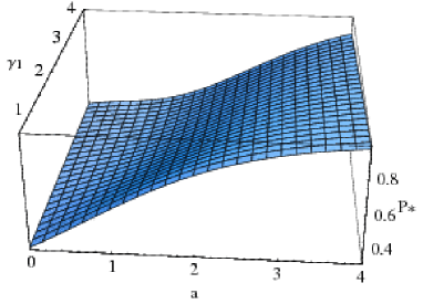
Figure 2: (Color online) Phase space surface of the steady state probability $\mathcal{P}_{A}^{*}$ that both units of a dimer are in the same state, indicating perfect synchronization, for $\gamma_{2}=0.5$ and a range of $\gamma_{1}$ and $a$.

The linear evolution equation of a single oscillator is $\partial P(t)/\partial t=MP(t)$, where the components $P_{i}(t)$ of the column vector $P(t)=(P_{1}(t)~{}P_{2}(t)~{}P_{3}(t))^{T}$ ($T$ denotes the transpose) are the probabilities of being in states $i=1,2,3$ at time $t$, and

$$M=\begin{pmatrix}-g&0&g\\ g&-g&0\\ 0&g&-g\end{pmatrix}.$$ (1)

The system reaches a steady state for $P_{1}^{*}=P_{2}^{*}=P_{3}^{*}=1/3$. The transitions $i\rightarrow i+1$ occur with a rough periodicity determined by $g$; that is, the time evolution of our simple model qualitatively resembles that of the discretized phase of a generic noisy oscillator with the intrinsic eigenfrequency set by the value of $g$.

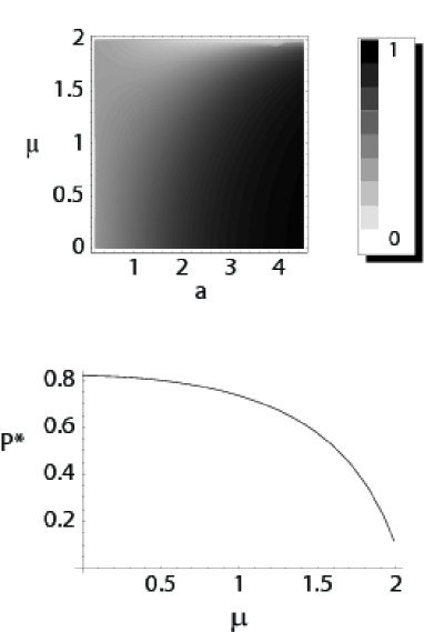
Figure 3: The steady state probability $\mathcal{P}_{A}^{*}$ that both units of a dimer are in the same state for a range of $\mu$ and $a$. Top: contour image. Bottom: a single curve for $a=2.2$. In the latter case, it is clear that as $\mu$ rises, synchronization rapidly decreases.

To study coupled arrays of these oscillators, we couple individual units by allowing the transition rates of each unit to depend on the states of the units to which it is connected. Specifically, for $N$ identical units we choose the transition rate of a unit $\nu$ from state $i$ to state $j$ as

$$g_{ij}=g\exp\left[{\frac{a(N_{j}-N_{i-1})}{n}}\right]\delta_{j,i+1},$$ (2)

where $\delta$ is the Kronecker delta, $a$ is the coupling parameter, $g$ is the transition rate parameter, $n$ is the number of oscillators to which unit $\nu$ is coupled, and $N_{k}$ is the number of units among the $n$ that are in state $k$. Each unit may thus transition to the state ahead or remain in its current state depending on the states of its nearest neighbors. In our earlier work we considered the globally coupled system, $n=N-1$, and also nearest neighbor coupling in square, cubic, or hypercubic arrays, $n=2d$ ($d=$ dimensionality). Here we focus on the globally coupled array.

Our previous work used a slightly different form of the coupling (2), with $N_{i-1}\to N_{i}$. While the differences in these details do not in any way affect the characterization of the synchronization transitions, that earlier choice was numerically advantageous because it led to a phase transition at a lower critical value $a_{c}$ of the coupling constant ($a_{c}=1.5$ in the globally coupled array) than other choices. A lower coupling in turn facilitates numerical integration of equations of motion because the time step that one needs to use near the phase transition must be sufficiently small, $dt\ll e^{-a}/g$. However, that earlier coupling choice brought with it a result that is undesirable in our present context (but was of no consequence before). In our earlier model, as the units become increasingly synchronized above the transition point, the average transition rate of a cluster becomes substantially dependent on the value of $a$; specifically, the transitions and cluster oscillation frequency slow as $a$ is increased due to an exponential decrease in the transition probability. To cite an explicit example, consider a small subsystem composed of units which are all in the same state at time $t$ (that is, a cluster of units which are perfectly synchronized). The previous form of the coupling yields an exponentially small transition rate in this case, and hence the oscillation frequency of this microscopic cluster approaches zero for high values of $a$. Since here we specifically wish to analyze the effects of transition rate disorder, it is desirable to deal with a model in which the average transition rate of identical synchronized units depends only on their intrinsic transition rate parameter and not on coupling strength. The form (2) reduces simply to the constant $g$ when the coupled units are perfectly synchronized. While the critical coupling in this new version is higher than in our earlier model and hence is numerically less efficient, no other features of the synchronization transition are affected. This in fact supports the desired insensitivity of the interesting macroscopic features of the model to microscopic modifications.

For a population of $N\to\infty$ identical units in the mean field (globally coupled) version of this model we can replace $N_{k}/N$ with the probability $P_{k}$, thereby arriving at a nonlinear equation for the mean field probability, $\partial P(t)/\partial t=M[P(t)]P(t)$, with

$$M[P(t)]=\begin{pmatrix}-g_{12}&0&g_{31}\\ g_{12}&-g_{23}&0\\ 0&g_{23}&-g_{31}\end{pmatrix}.$$ (3)

Figure 4: The steady state probability $\mathcal{P}_{A}^{*}$ that both units of a dimer are in the same state for $(\gamma_{1},\gamma_{2})=(0.5,1.5)$ as $a$ is increased (solid line). The points represent simulation results, where $\mathcal{P}_{A}^{*}$ is measured as the fraction of time that both units are fully synchronized.

Normalization allows us to eliminate $P_{3}(t)$ and obtain a closed set of equations for $P_{1}(t)$ and $P_{2}(t)$. We can then linearize about the fixed point $(P_{1}^{*},P_{2}^{*})=(1/3,1/3)$, yielding a set of complex conjugate eigenvalues which determine the stability of this disordered state. Specifically, we find that $2\lambda_{\pm}/g=(a-3)\pm i\sqrt{3}(1+a)$, eigenvalues that cross the imaginary axis at $a_{c}=3$, indicative of a Hopf bifurcation at this value. Note that the oscillation frequency of the array at the critical point as given by the imaginary parts of the eigenvalues is $\omega=\sqrt{3}g/2$. A more detailed analysis threestate1 ; threestate2 ; kuznetsov shows the bifurcation to be supercritical.

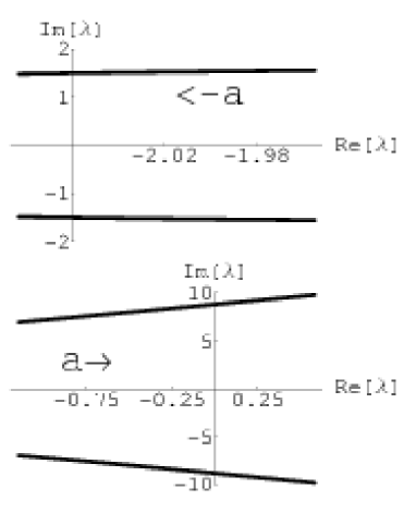
Figure 5: The two pairs of complex conjugate eigenvalues for the dichotomously disordered system, $\mathcal{N}=2$. Top panel: $(\lambda_{-},\lambda_{-}^{*})$. Bottom panel: $(\lambda_{+},\lambda_{+}^{*})$. The coupling constant is in the range $2.9\leq a\leq 4.5$, and the transition rate parameters are chosen to be $(\gamma_{1},\gamma_{2})=(1,3)$. In the bottom panel the critical value of $a$ is $a_{c}\approx 3.95$.

III Dimer

Consider first the simplest “disordered array,” namely, a mutually coupled dimer where one unit is characterized by $g=\gamma_{1}$ and the other by $g=\gamma_{2}$. In terms of the states (phases) $S_{1}$ and $S_{2}$ of units 1 and 2, there are 9 possible dimer states, $(S_{1},S_{2})=(1,1),(1,2),\ldots,(3,3)$, but it is not necessary to seek the ensemble distributions for all of these states in order to decide whether or not the two units are synchronized. We can directly write an exact reduced linear evolution equation for the $3$ states $A$, $B$, and $C$, where $A$ corresponds to any situation where both units are in the same state [that is, $(S_{1},S_{2})=(1,1),(2,2)$, and $(3,3)$], state $B$ corresponds to a situation where unit $1$ is one state “ahead” [$(S_{1},S_{2})=(2,1),(3,2)$, and $(1,3)$], and state $C$ corresponds to a situation where unit $2$ is one state “ahead” [$(S_{1},S_{2})=(1,2),(2,3)$, and $(3,1)$]. The evolution equation for these states is the closed linear set

$$\partial\mathcal{P}(t)/\partial t=\mathcal{A}\mathcal{P}(t),$$ (4)

with $\mathcal{P}(t)$ the time dependent probability column vector $(\mathcal{P}_{A}(t)~{}\mathcal{P}_{B}(t)~{}\mathcal{P}_{C}(t))^{T}$ and

$$\mathcal{A}=\begin{pmatrix}-\gamma_{1}-\gamma_{2}&b\gamma_{2}&b\gamma_{1}\\ \gamma_{1}&-b^{-1}\gamma_{1}-b\gamma_{2}&b^{-1}\gamma_{2}\\ \gamma_{2}&b^{-1}\gamma_{1}&-b\gamma_{1}-b^{-1}\gamma_{2}\end{pmatrix},$$ (5)

and where we have introduced the abbreviation

$$b\equiv e^{a}.$$ (6)

This evolution equation is easy to derive from the definition of the coupling, Eq. (2). For example, when the system is in state $A$, it can either go to state $B$, which happens when unit $1$ jumps ahead with transition rate $\gamma_{1}$, or it can go to state $C$, which happens when unit $2$ jumps ahead with transition rate $\gamma_{2}$. Similarly, when the system is in state $B$, it can either jump to state $A$ (when the lagging unit transitions forward) with transition rate $b\gamma_{2}$ or jump to state $C$ (when the leading unit transitions forward) with transition rate $b^{-1}\gamma_{1}$.

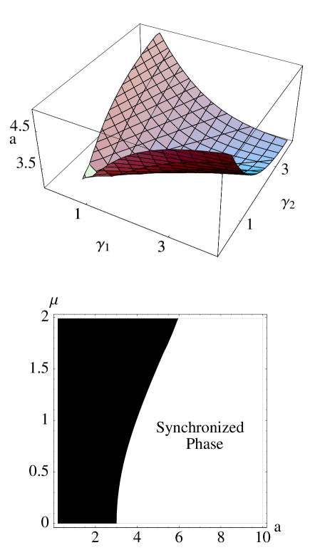
Figure 6: (Color online) Upper panel: Stability boundary for the dichotomously disordered system. The contour Re$\lambda_{+}=0$ is plotted in $(\gamma_{1},\gamma_{2},a)$ space. This contour indicates the critical point, where the Hopf bifurcation occurs and the disordered solution becomes unstable. The region above the contour represents the synchronized phase. Lower panel: Stability boundary in terms of relative width parameter.

With normalization, Eq. (4) becomes a $2$-dimensional equation having steady state solution

$$\mathcal{P}_{A}^{*} =\frac{b(\gamma_{1}^{2}+b^{2}\gamma_{1}\gamma_{2}+\gamma_{2}^{2})}{(1+b+b^{2})(\gamma_{1}^{2}+\gamma_{2}^{2})+(2+b^{3})\gamma_{1}\gamma_{2}},$$ (7)

$$\mathcal{P}_{B}^{*} =\frac{b^{2}\gamma_{1}^{2}+\gamma_{2}(\gamma_{1}+\gamma_{2})}{(1+b+b^{2})(\gamma_{1}^{2}+\gamma_{2}^{2})+(2+b^{3})\gamma_{1}\gamma_{2}}.$$

The eigenvalues of the two-dimensional matrix obtained from $\mathcal{A}$ after implementing normalization have negative real parts for all positive values of the parameters $a$, $\gamma_{1}$, and $\gamma_{2}$, indicating that the fixed points given by Eq. (7) are stable. Hence, the system asymptotically tends to this steady state solution. We are particularly interested in $\mathcal{P}_{A}^{*}$, the probablity for the system to be synchronized. In terms of the single relative width parameter width/mean,

$$\mu\equiv\frac{2(\gamma_{1}-\gamma_{2})}{(\gamma_{1}+\gamma_{2})}$$ (8)

($-2\leq\mu\leq 2$), this probability is

$$\mathcal{P}_{A}^{*}=\frac{b}{(2+b)}\left(\frac{1+\mu^{2}\frac{\displaystyle{(2-b^{2})}}{\displaystyle{4(2+b^{2})}}}{1+\mu^{2}\frac{\displaystyle{b(2+2b-b^{2})}}{\displaystyle{4(2+b^{2})(2+b)}}}\right).$$ (9)

The probability of synchronization for a dimer of identical units ($\mu=0$) is thus $\mathcal{P}_{A}^{*}=b/(2+b)=e^{a}/(2+e^{a})$, which increases with increasing coupling. This is the maximal syncrhonization; it is easy to ascertain that $\mathcal{P}_{A}^{*}$ decreases with increasing $\mu^{2}$, as one would anticipate. The full behavior of $\mathcal{P}_{A}^{*}$ as a function of the various parameters is shown in Figs. 2-4. The gradual increase in synchronization probability with increasing coupling turns into a sharp transition as a function of $a$ in the infinite systems to be considered below. The decreased synchronization probability when the frequencies of the two units become more dissimilar (increasing $\mu$) will also be reflected in the dependence of the critical coupling on transition rate parameter disorder.

IV $\mathcal{N}$ Different Transition Rates

Next we consider globally coupled arrays of oscillators that can have one of $\mathcal{N}$ different transition rate parameters, $g=\gamma_{u}$, $u=1,\ldots,\mathcal{N}$. To arrive at a closed set of mean field equations for the probabilities we again go to the limit of an infinite number of oscillators, $N\to\infty$. However, we must do so while preserving a finite density of each of the $\mathcal{N}$ types of oscillators. The probability vector is now $3\mathcal{N}$-dimensional, $P(t)=(P_{1,\gamma_{1}}~{}P_{2,\gamma_{1}}~{}P_{3,\gamma_{1}}~{}\cdots~{}P_{1,\gamma_{\mathcal{N}}}~{}P_{2,\gamma_{\mathcal{N}}}~{}P_{3,\gamma_{\mathcal{N}}})^{T}$. The added subscript on the components of $P(t)$ keeps track of the transition rate parameter. Explicitly, the component $P_{i,\gamma_{u}}$ is the probability that a unit with transition rate parameter $g=\gamma_{u}$ is in state $i$. The mean field evolution for the probability vector is the set of coupled nonlinear differential equations $\partial P(t)/\partial t=M_{\mathcal{N}}[P(t)]P(t)$, with

$$M_{\mathcal{N}}[P(t)]=\begin{pmatrix}\mathcal{M}_{\gamma_{1}}&0&\ldots&0\\ 0&\mathcal{M}_{\gamma_{2}}&\ldots&0\\ :&:&:&:\\ 0&\ldots&0&\mathcal{M}_{\gamma_{\mathcal{N}}}\end{pmatrix}.$$ (10)

Here

$$\mathcal{M}_{\gamma_{u}}=\begin{pmatrix}-g_{12}(\gamma_{u})&0&g_{31}(\gamma_{u})\\ g_{12}(\gamma_{u})&-g_{23}(\gamma_{u})&0\\ 0&g_{23}(\gamma_{u})&-g_{31}(\gamma_{u})\end{pmatrix},$$ (11)

and

$$g_{ij}(\gamma_{u})=\gamma_{u}\exp\left[a\sum_{k=1}^{\mathcal{N}}\varphi(\gamma_{k})\left(P_{j,\gamma_{k}}-P_{i-1,\gamma_{k}}\right)\right]\delta_{j,i+1}.$$ (12)

The function $\varphi(\gamma_{k})$ is the fraction of units which have a transition rate parameter $g=\gamma_{k}$.

As before, probability normalization allows us to reduce this to a system of $2\mathcal{N}$ coupled ordinary differential equations. It is interesting to compare this setup with that of the original Kuramoto problem with noise, where a continuous frequency distribution is introduced and the governing equation is a nonlinear partial differential equation [the Fokker-Planck equation for the density $\rho(\theta,\omega,t)$] acebron . The discretization of phase in our model results instead in a set of $2\mathcal{N}$ coupled nonlinear ordinary differential equations.

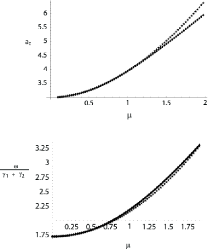
Figure 7: Upper panel: Critical coupling $a_{c}$ as a function of $\mu$ for a dichotomous ($\mathcal{N}=2$) array of globally coupled oscillators. The two curves represent the exact relationship (lower curve) and the small $\mu$ approximation (upper curve), respectively. Lower panel: The frequency of synchronous oscillation at the transition point. Lower curve is the approximation as predicted by ${\rm Im}\lambda_{+}$, upper curve is the exact result.

While it is nevertheless still difficult to solve these equations even for small $\mathcal{N}$, we can linearize about the disordered state $P(t)=(1/3~{}1/3~{}\ldots~{}1/3)^{T}$ and arrive at a $2\mathcal{N}\times 2\mathcal{N}$ Jacobian of the block matrix form

$$J=\begin{pmatrix}\mathcal{J}_{1}(\gamma_{1})&\mathcal{J}_{2}(\gamma_{1})&\mathcal{J}_{2}(\gamma_{1})&\ldots&\mathcal{J}_{2}(\gamma_{1})\\ \mathcal{J}_{2}(\gamma_{2})&\mathcal{J}_{1}(\gamma_{2})&\mathcal{J}_{2}(\gamma_{2})&\ldots&\mathcal{J}_{2}(\gamma_{2})\\ :&:&:&:&:\\ :&:&:&:&:\\ \mathcal{J}_{2}(\gamma_{N})&\mathcal{J}_{2}(\gamma_{N})&\ldots&\mathcal{J}_{2}(\gamma_{N})&\mathcal{J}_{1}(\gamma_{N})\end{pmatrix}.$$ (13)

The blocks $\mathcal{J}_{1}(g)$ and $\mathcal{J}_{2}(g)$ are given by:

$$\mathcal{J}_{1}(g)=\begin{pmatrix}-2g&-g-ag/N\\ g+ag/N)&-g+ag/N\end{pmatrix}$$ (14)

and

$$\mathcal{J}_{2}(g)=\begin{pmatrix}0&-ag/N\\ ag/N&ag/N\end{pmatrix}.$$ (15)

While we explore this in more detail below only for small $\mathcal{N}$, we note that in general the Jacobian (13) has $\mathcal{N}$ pairs of complex conjugate eigenvalues, only one pair of which seems to have a real part that becomes positive with increasing coupling constant $a$. This implies that there is a single transition to synchrony even in the presence of the transition rate disorder that we have introduced here. We go on to confirm this behavior for $\mathcal{N}=2$, $3$, and $4$.

IV.1 Two transition rate parameters

For the $\mathcal{N}=2$ case, the four eigenvalues $(\lambda_{+},\lambda_{+}^{*},\lambda_{-},\lambda_{-}^{*})$ of the Jacobian can be determined analytically. We find

$$\frac{{\rm Re}\lambda_{\pm}}{\gamma_{1}+\gamma_{2}} =\frac{1}{8}\left[a-6\pm B(a,\mu)\cos\left(C(a,\mu)\right)\right],$$ (16)

$$\frac{{\rm Im}\lambda_{\pm}}{\gamma_{1}+\gamma_{2}} =\frac{1}{8}\left[\sqrt{3}(a+2)\pm B(a,\mu)\sin\left(C(a,\mu)\right)\right],$$

where

$$B(a,\mu) \equiv\sqrt{2}\left[a^{4}-6a^{2}\mu^{2}+3\mu^{4}(a^{2}+3)\right]^{1/4},$$ (17)

$$C(a,\mu) \equiv\frac{1}{2}\tan^{-1}\left(\frac{-\sqrt{3}(a^{2}-(a+3)\mu^{2})}{a^{2}+3(a-1)\mu^{2}}\right).$$

Aside from an overall factor $(\gamma_{1}+\gamma_{2})$, Eqs. (16) depend only on the relative width variable as defined in Eq. (8), and therefore the critical coupling $a_{c}$ depends only on $\mu$. As illustrated in Fig. 5, one pair of eigenvalues crosses the imaginary axis at a critical value $a=a_{c}$, but the other pair shows no qualitative change as $a$ is varied. While this figure shows only the particular transition rate parameter values $(\gamma_{1},\gamma_{2})=(1,3)$, the qualitative features of these eigenvalues remain similar for the entire range of positive parameters. The upper panel of Fig. 6 depicts the contour Re$\lambda_{+}=0$ in $(\gamma_{1},\gamma_{2},a)$ space; this contour represents the critical surface and thus separates the synchronous and disordered phases.

The critical coupling is the value of $a$ at which Re$\lambda_{+}=0$ (Re$\lambda_{-}$ does not vanish for any $a$). It is easy to ascertain that Im$\lambda_{+}$ does not vanish at $a_{c}$, so that the critical point is a Hopf bifurcation. Furthermore, it is clear from Eq. (16) that $a_{c}$ depends only on the relative width parameter $\mu$, and it is also straightforward to establish that $a_{c}$ increases with increasing $\mu$, that is, a stronger coupling is necessary to overcome increasingly different values of $\gamma_{1}$ and $\gamma_{2}$ (see lower panel of Fig. 6). Note, however, that the dependence on $\mu$ implies that it is not just the difference in transition rates but the relative difference or percent difference relative to the mean transition rate that is the determining factor in how strong the coupling must be for synchronization to occur. A small-$\mu$ expansion leads to an estimate of $a_{c}$ to $O(\mu^{2})$,

$$a_{c}\approx\frac{1}{8}\left(12+3\mu^{2}+\sqrt{3}\sqrt{(12+\mu^{2})(4+3\mu^{2})}\right),$$ (18)

a result that exhibits these trends explicitly. The upper panel in Fig. 7 shows that this estimate is remarkably helpful even when $\mu^{2}$ is not so small.

The frequency of oscillation of the synchronized system at the transition is given by $\omega=\lim_{a\to a_{c}}$Im$\lambda_{+}$. From Eq. (16) it follows that $\omega$ depends on $(\gamma_{1}+\gamma_{2})$ as well as $\mu$. The small-$\mu$ expansion leads to the estimate

$$\omega=Im(\lambda_{\pm})|_{a\to a_{c}}\approx\frac{1}{4}\sqrt{3}(\gamma_{1}+\gamma_{2})(4+\mu^{2}),$$ (19)

which works exceedingly well for all $\mu$ (see Fig. 7).

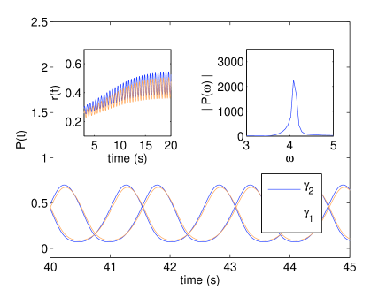
Figure 8: (Color online) The components $P_{1,\gamma_{1}}$ and $P_{2,\gamma_{1}}$(two lighter or brown curves), and $P_{1,\gamma_{2}}$ and $P_{2,\gamma_{2}}$(two darker or blue curves), of the vector $P(t)$ vs time for $\gamma=1,~{}\Delta=0.125$, with $a=3.15$, which is above the critical value $a_{c}\approx 3.02$ predicted by linearization. The left inset shows the order parameter $r(t)$ as it approaches its long-time limit. The right inset shows the frequency spectrum of a component of $P(t)$. The spectrum has a dominant peak near $\omega\approx 4$, and is expected to approach the frequency $\omega\approx 3.5$ predicted by linearization as we approach the transition point $a\to a_{c}$.

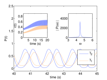
Figure 9: (Color online) The components $P_{1,\gamma_{1}}$ and $P_{2,\gamma_{1}}$(two lighter or brown curves), and $P_{1,\gamma_{2}}$ and $P_{2,\gamma_{2}}$(two darker or blue curves), of the vector $P(t)$ vs time for $\gamma=1,~{}\Delta=0.625$, with $a=3.5$, which is above the critical value $a_{c}\approx 3.39$ predicted by linearization. The left inset shows the order parameter $r(t)$ as it approaches its long-time limit. The right inset shows the frequency spectrum of a component of $P(t)$. The spectrum has a dominant peak near $\omega\approx 4.4$, and is expected to approach the frequency $\omega\approx 3.8$ predicted by linearization as we approach the transition point $a\to a_{c}$.

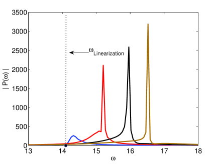
Figure 10: (Color online) The frequency $\omega$ of macroscopic oscillations approaches the value predicted by linearization as $a\to a_{c}$. Here we have used $\gamma_{1}=3.5$ and $\gamma_{2}=4.5$ so that $\gamma=4$ and $\Delta=1$. The critical coupling constant is $a_{c}=3.06$. From darkest or blue to lightest or brown: $a=3.07$, $3.10$, $3.15$, and $3.20$.

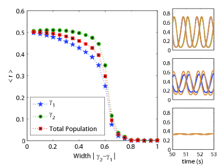
Figure 11: (Color online) Time-averaged order parameter $r$ in the long-time limit vs $\Delta$ for the individual oscillator populations characterized respectively by the transition rate parameter $\gamma_{1}$ (stars) and $\gamma_{2}$ (circles), and for the entire mixed array (squares). The insets show the time evolution of the probability vector components $P_{1,\gamma_{1}}$ and $P_{2,\gamma_{1}}$ (lighter or brown curves) and $P_{1,\gamma_{2}}$ and $P_{2,\gamma_{2}}$ (darker or blue curves) for widths 0.05 (upper inset), 0.5 (middle inset), and 0.9 (lower inset). Some of the curves are not visible because they are so perfectly superimposed. While the degree of synchronization varies within each population, the critical width for de-syncrhonization is the same for both, as predicted by linearization. The coupling constant for all cases is $a=3.2$ and the average transition rate parameter $\gamma=1.5$.

To check the predictions of our linearization procedure, we numerically solve the nonlinear $\mathcal{N}=2$ mean field equations. In agreement with the structure of the linearized eigenvalues, all components of $P(t)$ synchronize to a common frequency as the phase boundary in $(\mu,a)$-space) is crossed. Interestingly, the numerical solutions also give us insight into the amplitude of the oscillations; that is, they allow us to explore the relative “magnitude” of synchronization within the two populations. As we will see, the two populations indeed oscillate with the same frequency, but with amplitudes and “degrees of synchronization” that can be markedly different. Consider the order parameter $r(t)$ given by

$$r(t)\equiv\frac{1}{N}\left\lvert\sum_{\nu=1}^{N}e^{i\phi_{\nu}}\right\rvert.$$ (20)

Here $\phi_{\nu}$ is the discrete phase 2$\pi$($k$-1)/3 for state $k\in\{1,2,3\}$ at site $\nu$. For phase transition studies, one would likely average this quantity over time in the long time limit, and also over independent trials. For our purposes here, though, we find the time-dependent form more convenient. In the mean field case, where we solve for probabilities to be in each state, the order parameter is easily calculated by writing the average in Eq. (20) in terms of these probabilities rather than as a sum over sites.

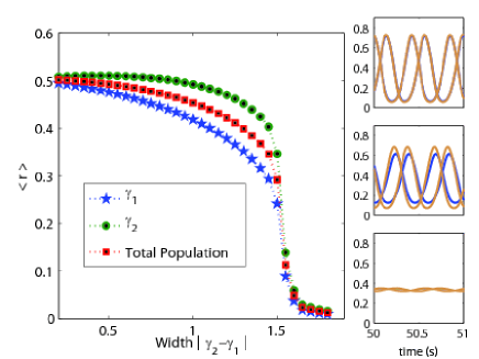
Figure 12: (Color online) Same as Fig. 11 but with $\gamma=3.5$ and widths 0.1 (upper inset), 1.3 (middle), and 1.8 (lower).

In subsequent figure captions we introduce the notation $\gamma\equiv(\gamma_{1}+\gamma_{2})/2$ (average transition rate parameter), and the difference $\Delta\equiv|\gamma_{2}-\gamma_{1}|$ (note that $\mu=\Delta/\gamma$). As shown in Figs. 8-12, the predictions of linearization accurately describe the onset of macroscopic synchronization and provide an estimation of the frequency of these oscillations near threshold (see Fig. 10). Specifically, Figs. 8 and 9 show the macroscopic oscillations for coupling $a$ above threshold. All the oscillators, regardless of their intrinsic transition rate parameter, oscillate exactly in phase, but the degree of synchronization is greater in the population with the larger $\gamma_{i}$ (here $\gamma_{2}$), as evidenced by the unequal amplitude of the components of $P(t)$ for the two populations. The “greater degree of synchronization” is also apparent in the order parameter $r(t)$ shown in the insets, which is larger for the oscillators with the higher intrinsic transition rate. These results support the notion that populations with higher transition rate parameters in some sense synchronize more readily. The figures also show the frequency spectrum of any component of $P(t)$. The peak occurs at the frequency of oscillation of the synchronized array. As $a\to a_{c}$ this frequency approaches the value Im$\lambda_{+}$ predicted by linearization, as shown in Fig. 10.

Figures 11 and 12 illustrate the sudden de-synchronization (at fixed $a$ and $\gamma$) accompanying an increase in the difference $\Delta$. This behavior is reminscent of that of the original Kuramoto oscillators, which become disordered as the width of the frequency distribution characterizing the population exceeds some critical value. The insets show the components of $P(t)$ and confirm that both populations undergo the de-syncrhonization transition at the same critical value of the difference $\Delta$. Comparing the two figures, we see that the system with a higher average transition rate parameter (Fig. 12) can withstand a larger difference $\Delta$ before de-syncrhonization, again confirming our earlier observations.

One last point to consider is the relation between the frequency of oscillation of the synchronized array above $a_{c}$ and the frequencies of oscillation of the two populations if they were decoupled from one another. As coupling increases, the oscillation frequency $\omega$ moves closer to that of the population with the lower transition rate parameter. This is illustrated in Fig. 13 for the same parameters used in Fig. 10.

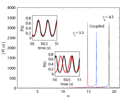
Figure 13: (Color online) Frequency spectra of the numerical solutions to the mean field equations ($\mathcal{N}=2$) show that above critical coupling, $a=3.2>a_{c}=3.06$, synchronization occurs at a frequency closer to the lower of the two population frequencies. Top left inset: $P_{1,\gamma_{1}=3.5}$ and $P_{1,\gamma=4.5}$ when all units are globally coupled. Bottom right inset: the same curves for populations that are uncoupled from one another (but still globally coupled within each population).

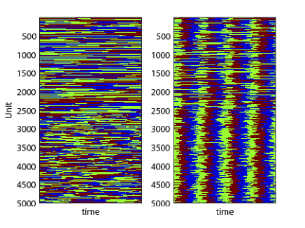
Figure 14: (Color online) Long-time snapshots of a globally coupled system above and below threshold. In both cases, $(\gamma_{1},\gamma_{2})=(0.5,1.5)$. On the left, $a=3.5<a_{c}$ while on the right, $a=4.1>a_{c}$. In both cases, all units are globally coupled. For visualization purposes, the plot is arranged so that population $\gamma_{1}$ consists of the first $2500$ units (the top), while population $\gamma_{2}$ consists of the second $2500$ units (the bottom). Global synchrony emerges for $a>a_{c}$. In addition, the population with the higher transition rate parameter is more synchronized.

Finally, a visually helpful illustration of these behaviors is obtained via a direct simulation of an array with a dichotomous population of oscillators. Since our oscillators are globally (all-to-all) coupled, the notion of a spatial distribution is moot, and for visulatization purposes we are free to arrange the populations in any way we wish. In Fig. 14 we display an equal number of $\gamma_{1}$ and $\gamma_{2}$ oscillators and arrange the total polulation of $N=5000$ so that the first 2500 have transition rate parameter $\gamma_{1}$ and the remaining 2500 have transition rate parameter $\gamma_{2}$. In this simulation we have chosen $\gamma_{1}=0.5$ and $\gamma_{2}=1.5$, so that $\gamma=\Delta=1$. Although $N=5000$ is not infinite, it is large enough for this array to behave as predicted by our mean field theory. The left panel shows snapshots of the phases (each phase is indicated by a different color) when $a<a_{c}$ and the phases are random. The right panel shows the synchronized array when $a>a_{c}$. Clearly, all units are synchronized in the right panel, but the population with the higher transition rate parameter (lower half) shows a higher degree of synchronization (higher $P(t)$) as indicated by the intensity of the colors or the gray scale.

Figure 15: $\mathcal{N}=3$ case: The three pairs of complex conjugate eigenvalues are plotted in the complex plane for $2.9\leq a\leq 4.5$. The transition rate parameters are chosen to be $(\gamma_{1},\gamma_{2},\gamma_{3})=(1,2,3)$. In the bottom panel the critical value of $a$ is $a_{c}\approx 3.6$.

IV.2 $\mathcal{N}=3$ and $\mathcal{N}=4$

We can carry out this analysis, albeit not analytically (at least in practice), for any $\mathcal{N}$. We have explored the cases $\mathcal{N}=3$ and $4$. In both cases there appears to be only one pair of eigenvalues whose real parts can become positive, suggesting that synchronization occurs all at once and not in one population at a time (Figs. 15 and 16). This occurs no matter the distribution of the 3 or 4 transition rate parameters. For example, in the $\mathcal{N}=4$ case we have compared in some detail the cases where the four transition rates are equidistant and where they are pairwise much closer than the separation between the highest and lowest. In both cases there is a single transition to synchrony, albeit not at exactly the same value of $a_{c}$, indicating a more complex dependence on the transition rate parameter distribution than just via its mean and width. Furthermore, the basic trends of the dichotomous case broadly carry over, mainly in that the critical value $a_{c}$ increases when the width of the distribution increases relative to the mean (as one would expect). On the other hand, the inclusion of more transition rates within a given range leads to a lowering of the critical coupling. Thus, for example, the mean transition rate $\gamma$ and the width $\Delta$ are the same in the cases shown in Figs. 5 and 15 ($\gamma=\Delta=2$), and yet $a_{c}$ is higher in the former (3.95 for $\mathcal{N}=2$) than in the latter (3.6 for $\mathcal{N}=3$). Still, the mean and width of the distribution provide a rough qualitative assesment of the behavior, particularly for the case of a uniform distribution, which we study below.

Figure 16: $\mathcal{N}=4$ case: The four pairs of complex conjugate eigenvalues are plotted in the complex plane for $2.9\leq a\leq 4.5$. The transition rate parameters are chosen to be $(\gamma_{1},\gamma_{2},\gamma_{3},\gamma_{4})=(1,2,3,4)$. In the bottom panel, the critical value of $a$ is $a_{c}\approx 3.75$.

V Uniform Distribution of Transition Rate Parameters

We now turn to globally coupled arrays where the transition rate parameter $g$ for each unit is chosen from a uniform distribution over a finite interval, $\varphi(g)$. While it is difficult to make direct analytical progress in this general case, the earlier dimer analysis and the arrays of $\mathcal{N}=2,3,4$ different populations of units provide a framework for understanding the properties of these more general systems. In particular, the earlier results suggest that this “more disordered” system may also display a single transition to synchronization. To explore these and other features in more detail, we simulate $N=5000$ globally connected units characterized by the transition rate parameter distribution $\varphi(g)$, and we make several observations. Firstly, we do observe a single transition to macroscopic synchronization. Secondly, as suggested by the dichotomous case, synchronization appears more readily (that is, for a lower value of $a$) if the distribution $\phi(g)$ has a larger mean and smaller width. When the mean and width are varied independently, the qualitative trends from the dichotomous case are observed here as well. Thirdly, while synchronization in this system is again governed primarily by the mean and width of the distribution $\varphi(g)$, the critical value $a_{c}$ is considerably lower than that of the finite $\mathcal{N}$ systems with the same mean and width (as expected).

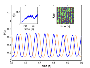
Figure 17: (Color online) The probability that the synchronized array is in state 1 (lighter or brown) and state 2 (darker or blue) as a function of time for a uniform distribution $\varphi(g)$ on the interval $[1.5,2.5]$ and coupling parameter $a=3$. Insets show the order parameter $r(t)$ as well as time resolved snapshots of the system.

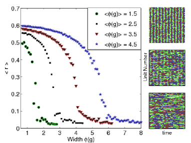
Figure 18: (Color online) As the width of the $\phi(g)$ distribution increases, a critical width is reached beyond which synchronization is destroyed. The coupling is chosen to be $a=3.2$, and the four curves represent the steady state, time-averaged order parameter for distributions with different means. As the mean of the $\phi(g)$ distribution increases, the transition to disorder occurs at a greater width. The insets at the right show the long-time behavior of an entire population of mean transition rate parameter 3.5 (corresponding to the triangle order parameter data) and widths of $0.6$, $4.0$, and $6.2$.

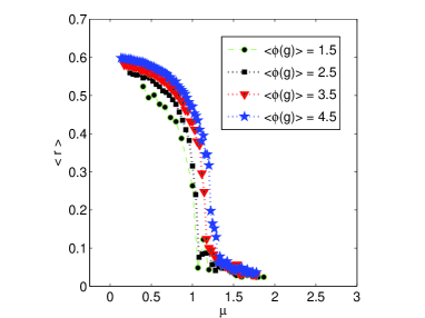
Figure 19: The data of Fig. 18 against the relative width $\mu$.

Two examples of our simulation results are shown in Figs. 17 and 18. In Fig. 17 we present the first two components of the 3-dimensional vector $P(t)$ whose components $P_{i}(t)$ represent the probability that all units of the entire synchronized array are in state $i$. The probabilities $P_{1}(t)$ and $P_{2}(t)$ oscillate in time with essentially constant amplitude and a constant relative phase, indicating global synchronization. The upper left inset shows the order parameter $r(t)$ and the upper right inset the time resolved snapshot of the system, both indicating a high degree of synchronization. Note that the coupling parameter $a=3$ in the figure is below the critical value $a_{c}=3.2$ for the dichotomous case with the same mean and width.

Figure  18 shows the steady state time-averaged order parameter $r$ at constant $a$ as the width of the $\phi(g)$ distribution is increased for a fixed mean. Similar to the $\mathcal{N}=2$ population case, synchronzation is destroyed as the width eclipses some critical value, and that value increases as the mean of the distrubtion increases. In Fig. 19 we plot the data from Fig 18 as a function of the relative width parameter $\mu$. Recalling that for the dichotomous array as well as for the dimer synchronzation at a given $a$ depends only on $\mu$, we might expect that the transition point $\mu_{c}$ (at constant $a$) is not significantly mean-dependent, even when there is a distribution of transition rate parameters. In fact, we can see that the curves approximately collapse onto one curve, indicating that the relative width $\mu$ provides a useful control parameter for predicting synchronization. Hence, the predictions of the linearization analysis for the $\mathcal{N}=2$ case provides qualitatively insight into the behavior of the disordered population.

VI Discussion

We have presented a discrete model for globally coupled stochastic nonlinear oscillators with a distribution of transition rate parameters. Our model exhibits a range of interesting dynamical behavior, much of which mimics the qualitative features of the canonical Kuramoto oscillator kuramoto , but with a mathematically and numerically considerably more tractable model. Since our phase variable is discrete (whereas the phase variable in the canonical problem is continuous), a distribution of $\mathcal{N}$ different transition rates in our array leads to a set of $2\mathcal{N}$ coupled nonlinear ordinary differential equations instead of a single partial differential equation for the probability distributions of interest. Linearization of our model around the critical point leads to a problem which at least for small $\mathcal{N}$ (specifically, for the dichotomous disorder case) becomes analytically tractable. Distributions involving a large finite number of transition rate parameters, while not easily amenable to analytic manipulation even upon linearization, reduce to a simple matrix algebra problem. For any distribution of transition rate parameters, even continuous, the model is in any case readily amenable to numerical simulation.

Our most salient conclusion is that such disordered globally coupled arrays of oscillators, even in the face of transition rate parameter disorder, undergo a single transition to macroscopic synchronization. Furthermore, we have shown that the critical coupling $a_{c}$ for synchronization depends strongly (but not exclusively) on the width $\Delta$ and mean $\gamma$ of the transition rate parameter distribution, specifically via the relative width $\mu=\Delta/\gamma$. This general feature is already apparent in the synchronization behavior of a dimer of two oscillators with transition rate parameters $\gamma_{1}$ and $\gamma_{2}$. An infinite array of two populations of oscillators, one with transition rate parameter $\gamma_{1}$ and the other with $\gamma_{2}$, displays a Hopf bifurcation, with $a_{c}$ determined solely by $\mu$. While a quantitative prediction of synchronization on the basis of the relative width is not possible in all cases, it does determine qualitative aspects of the transition for more complex transition rate parameter distributions. We have explored this assertion for arrays with $\mathcal{N}=2,~{}3,$ and $4$ and with a uniform distribution of transition rates over a finite interval, and expect it be appropriate for other smooth distributions as well.

A number of further avenues of investigation based on our stochastic three-state phase-coupled oscillator model are possible. For example, we could explore the effects of transition rate disorder in locally coupled arrays whose behavior we have fully characterized for identical oscillators threestate1 ; threestate2 . It would be interesting to explore the consequences of disorder in the coupling parameter $a$. Finally, we note that a two-state version of this model (which of course does not lead to phase synchronization as discussed here) has recently been shown to accurately capture the unique statistics of blinking quantum dots grigolini . Such wider applicability of the model, together with its analytic and numerical tractability, clearly opens the door to a number of new directions of investigation.

References

- (1) S. H. Strogatz, Nonlinear Dynamics and Chaos (Westview Press, 1994).
- (2) A. T. Winfree, J. Theor. Biol. 16, 15 (1967).
- (3) Y. Kuramoto, Chemical Oscillations, Waves, and Turbulence (Springer, Berlin, 1984).
- (4) S. H. Strogatz, Physica D 143, 1 (2000).
- (5) A. Pikovsky, M. Rosenblum, J. Kurths, Synchronization: A Universal Concept in Nonlinear Science (Cambridge University Press, Cambridge, 2001).
- (6) T. Prager, B. Naundorf, and L. Schimansky-Geier, Physica A 325, 176 (2003).
- (7) H. Sakaguchi, S. Shinomoto, and Y. Kuramoto, Prog. Theor. Phys. 77, 1005 (1987); H. Daido, Phys. Rev. Lett. 61, 231 (1988); S. H. Strogatz and R. E. Mirollo, J. Phys. A 21, L699 (1988); idem, Physica D 31, 143 (1988); H. Hong, H. Park, and M. Choi, Phys. Rev. E 71, 054204 (2004).
- (8) K. Wood, C. Van den Broeck, R. Kawai, and K. Lindenberg, Phys. Rev. Lett. 96, 145701 (2006).
- (9) K. Wood, C. Van den Broeck, R. Kawai, and K. Lindenberg, Phys. Rev. E 74, 031113 (2006).
- (10) T. Risler, J. Prost, F. J ulicher. Phys. Rev. Lett. 93, 175702 (2004).
- (11) T. Risler, J. Prost, and F. J ulicher, Phys. Rev. E 72, 016130 (2005).
- (12) Yu. A. Kuznetsov, Elements of Applied Bifurcation Theory, 2nd ed. (Springer, New York, 1998).
- (13) Acebron, J., L. Bonilla, C. Perez Vicente, F. Ritort, and R Spigler. Rev. Mod. Phys. 77, (2005).
- (14) S. Bianco, E. Geneston, P. Grigolini, and M. Ignaccolo, arXiv:cond-mat/0611035 (2006).