Trapping electrons in electrostatic traps over the surface of 4He.

Abstract

We have observed trapping of electrons in an electrostatic trap formed over the surface of liquid ${}^{4}\mathrm{He}$. These electrons are detected by a Single Electron Transistor located at the center of the trap. We can trap any desired number of electrons between 1 and $\sim 30$. By repeatedly ($\sim 10^{3}-10^{4}$ times) putting a single electron into the trap and lowering the electrostatic barrier of the trap, we can measure the effective temperature of the electron and the time of its thermalisation after heating up by incoherent radiation.

In 1999, Platzman and Dykman[1] proposed that single electrons electrostatically trapped on the surface of a liquid helium film could be used as qubits and hence form the basis of a quantum computer. This proposal quickly aroused experimentalists’ interest.[2] Here we present experimental results on the trapping of a single (or other desired number) electron and measurements of the upper limit of its relaxation time in view of defining its usefulness as potential qubit.

1 The experiment

The tested device consists in a system of electrodes designed to hold an electron in a well-defined position over the liquid helium surface. A single electron transistor (SET) located below the electron is used to monitor its quantum state. The whole structure is represented in Fig. 1. It comprises an electron reservoir and the electron trap, which is supplied in electrons from the reservoir, and a guard electrode made out of a thick ($\sim$0.5 $\mu$m) layer of Nb. The structure is covered by a saturated helium film $\sim$200-400 Å in thickness. Two electrodes, made out of thin Niobium and lying at the bottom of the reservoir, fix its electrostatic potential with respect to the guard.

A gorge through the guard electrode connects the reservoir to the trap. When this electrode is negatively biased relative to the SET, a potential barrier forms at this gorge, isolating the trap from the reservoir.

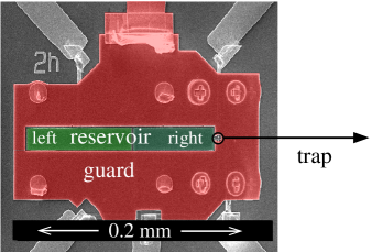
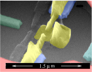
Figure 1: Scanning Electron Microscope photograph of the microfabricated part of the sample (left) and the electron trap (right). (color online)

The voltage across the SET is modulated by the charge on its island, $q_{I}=\sum_{i}{C_{i}U_{i}}+\sum_{j}{q_{0,j}}$. The first sum is over all the conductors in the systems having capacitance $C_{i}$ and potential $U_{i}$ with respect to the island. The second sum is over the image charges induced on the island by stray charges in the rest of the system, such as charges or dipoles in the substrate and the electrons over helium. The voltage $V_{s}(q_{I})$ is a priori unknown. It depends on the bias current and changes from run to run. However, it must be periodic with period $e$, the charge of the electron.

To reduce the noise due to fluctuations of the dc voltage across the SET, we apply a low-frequency (80-150 Hz) modulation of the order of 100 $\mu$V to the guard electrode, which is strongly coupled to the SET island. The voltage variation across the SET produced by this modulation is detected by a lock-in amplifier. The amplitude of this signal $V(q_{I})$ is proportional to the derivative of $V_{s}(q_{I})$ function and, thus, is periodic itself. We determine $V(q_{I})$ experimentally by sweeping the potential, $U_{e}$, of one of the electrodes, usually the one which will be swept in subsequent measurements. We then choose a part of the response to the sweep where background charges did not change, so that several periods of the function $V(q_{I})=V(U_{e})$ can be superimposed by transforming $U_{e}$ modulo $P$, where the period $P$ is adjusted self-consistently. After the modulo transformation the chunk of data is averaged and interpolated by a smoothing spline function $\mbox{spl}(U_{e})$. The rest of the data is fitted piecewise with the function $A\cdot\mbox{spl}(U_{e}+qP)$, where the amplitude $A$, and the phase $q$ are the fitting parameters. Parameter $q$ is the charge, expressed as fraction of $e$, induced on the SET island by stray charges in the system.

An electron seeding and monitoring experiment proceeds as follows.

1. We seed the electrons on the helium surface by igniting a corona discharge in a small chamber separated from the rest of the cell by a transmission electron microscope sample grid. The cell is heated to $\sim$1.1 K before a discharge. The presence of the electron normally is easily detected by applying a voltage $U_{exc}\sim$100 $\mu$V at 100 kHz to the right reservoir electrode and measuring with a lock-in amplifier the voltage induced on the left electrode. When electrons appear on the surface, the signal changes by 10 to 200 nV rms.

2. After electrons are seeded, we let the system cool down from 1 K and proceed to trap the desired number of them in the trap. Typically, at this point, the guard electrode is biased to a negative potential, between $-0.1$ and $-0.5$ V, and the SET is biased to a positive potential between 0 and $0.5$ V. First, we lower the voltage applied to the reservoir electrodes to charge the trap. Care should be taken not to lower the voltage too much, since this can cause irreversible loss of all the electrons. Normally, we find the suitable potentials by trial and error. In typical cases, at least one of the reservoir electrodes stays more positive than the guard, although the electrons can be kept even with both electrodes negative with respect to the guard.

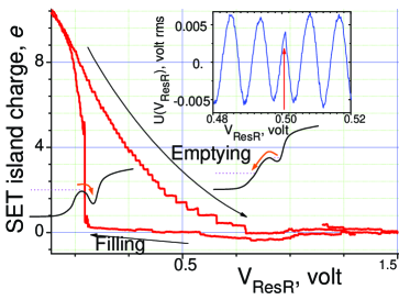
Figure 2: Reduced charge on the SET island in terms of the potential of the right reservoir electrode. SET potential is +0.6 V, Guard electrode potential 0. The bottom insert schematically shows calculated profile of the potential along the centerline of the sample, the dashed line schematically represents local energy of the electrons. The top insert shows small portion of a raw SET signal containing one of the jumps (indicated by the arrow). (color online)

3. After the trap is charged, we start ramping up the potential of the right reservoir electrode. Typical results are shown in Fig. 2, where we show the dependence of the phase of the SET signal oscillations on the voltage applied to that electrode. When we sweep the voltage from large positive values down, the charge induced on the SET changes little, until we reach the charging voltage. Small changes seen in Fig. 2 are probably due to motion of charges and dipoles in the substrate and occur even before the electrons are seeded for the first time after cooldown from room temperature. At the charging voltage ($\sim$0.26 V in the figure) the SET detects a sudden change in the charge. Since a SET measures charge modulo $e$, we can not determine the real change and adjust it by integer number of $e$ to “close the loop”.

The scheme of distribution of potentials at the moment of charging is shown in the insert of Fig. 2. The solid line represents the potential created by the electrodes along the center of symmetry of the sample in the plane of the electrons. The dashed line indicates the energy of the electrons, which, due to Coulomb repulsion, is higher than this potential by $ned/\varepsilon\varepsilon_{0}$, where $n$ is the electron number surface density and $d$ is their distance from the electrode.

When ramping down the potential, the energy of the electrons over the reservoir drops, but electrons in the potential well stay trapped. As the voltage on the right reservoir electrode is raised further, the barrier height decreases and electrons start leaking out one by one. Each electron leaving the trap monitored on the SET signal as a sudden change in the phase of the oscillations, shown in the top insert. Finally, at $\sim$0.63 V the last electron leaves the trap. Between $\sim$0.57 and $\sim$0.63 V only one electron is left in the trap.

The amplitude of the jump depends on the number of the electrons residing in the trap and goes to $\sim 0.4e$ for a few electrons. This value is to be compared with $\sim 0.5e$ obtained from the numerical simulation. The length of the plateaus between the jumps depend on the Coulomb repulsion between the electrons.

These results are rather similar to the results of the Royal Holloway group[3]. However, in the present experiments, the steps are more stable and better defined, being both “higher” and “longer”, because of the enhanced coupling to the pyramidal SET, compared with the flat-island SET and the smaller trap used in London.

2 Electron escape

Having developed the technique of trapping the electrons, we proceeded to the measurement of their escape from the trap. Having prepared the trap with one electron, we momentarily open it partially by applying short ($\sim 0.1\mu$s) pulses to the right reservoir electrode. We then examine the SET signal to determine the presence of the electron. If it has escaped, we re-populate the trap and repeat the measurement. After accumulating $\sim 1000$ attempts, we plot the resulting electron escape probability vs. the amplitude of the pulse opening the trap, as shown in Fig. 3. The error bars on the figure come from the statistical analysis of the data.

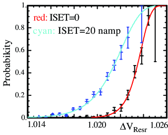
Figure 3: The probability of the escape of a single electron from a trap, in terms of the amplitude of the pulse applied to the right reservoir. Error bars and fits are discussed in the text. $V_{set}=+0.6$ V, $V_{gate}=+0.0$ V, $V_{guard}=-0.1$ V. The calculated potential barrier, used in the fit is $(0.16\cdot\mbox{volt})(V_{ResR}/\mbox{volt}-1.042)^{1.6}$. (color online)

The dependence of the escape probability from a potential well on some parameter can be calculated as in Ref.[Varoquaux:2003]: $p=1-\exp(-\mathit{\Gamma}\tau e^{-E(U)/kT})$, where $\mathit{\Gamma}$ is the attempt frequency of the escape, $\tau$ is the pulse length and $E(U)$ is the height of the energy barrier, which depends on parameter $U$. This formula applies also to the case of quantum tunneling through a barrier if it can be approximated by cubic+parabolic potential. In this case one should use the effective temperature $k_{B}T_{q}=\hbar\omega_{t}/2\pi$, where $\omega_{t}$ is the frequency of the oscillations of the particle in the well.

We have calculated the barrier height in terms of the voltage on the right reservoir numerically, using the known sample geometry. To account for possible contact potentials between electrodes, we have assumed that at the lowest temperature the escape of the electron is due to quantum tunneling. Then the calculated probability of escape has been fitted to the data with the SET potential as the fitting parameter. Here, we did not make assumption about the shape of the potential; calculated profiles of the potential barrier have been used. Using this adjusted value of the SET potential, the $E(V_{ResR})$ function is computed, which is then used in the subsequent fits. The fits are quite insensitive to the values of the attempt frequency and the pulse length, so we have used the fixed numbers of 40 GHz and $0.1\ \mu$s, correspondingly.

3 The electron temperature

The escape curve changes as a function of the current through the SET. To make this measurement, we apply the desired current to the SET, apply the measuring pulse to the right reservoir and then change the SET current to a value suitable for measurements ($\sim$3 nA). When the current through the SET is increased, the curve shifts to the left and becomes less steep. Both effects can be explained by an increase of the electron temperature. Such an increase is not surprising since the current through SET generates an electric field in its vicinity as electrons tunnel into and out of the island, changing the potential of the island by $\sim e/(2C_{\Sigma})$, where $C_{\Sigma}$ is the total capacitance of the island. Knowing the barrier, we can calculate the temperature of the electron from the fitting parameters. We find that the temperature of the electron at zero current through the SET is 270 mK, rising to 0.4 K at $I_{SET}=20$ nA while the cell temperature is $\sim\,$13 mK. Finally, when raising the cell temperature above 270 mK, we observe that the temperature of the electron increases more slowly than that of the cell.

Also, we tried to estimate the thermalisation time of the electron. After heating the electron by $I_{SET}$ we turn off the current and, after a delay, apply the measuring pulse. We determine the electron temperature by repeating the measurement a number of times and using the procedure outlined above. We find that the temperature always returns to a stationary value even for the shortest time delay that we could apply of $\sim 0.5\mu$s.

Both the anomalous behavior of the electron temperature and its short thermalisation time indicate a rather strong coupling with parts of the environment. We suspect that these features are due to the strong coupling with the pyramidal SET and by the large pressing field acting on the electrons.

References

- [1] P.M.Platzman and M.I.Dykman, Science 284, 1967 (1999).
- [2] M.J. Lea, P.G. Frayne, and Yu. Mukharsky, Fortschr. Phys. 48, 1109 (2000).
- [3] P. Glasson, G. Papageorgiou, K. Harrabi, et al., J. Physics and Chemistry of Solids 66, 1539 (2005).
- [4] E. Varoquaux and O. Avenel, Phys .Rev. B 68, 054515 (2003).