A detailed analysis of dipolar interactions and analytical approximations in arrays of magnetic nanowires

Abstract

The investigation of the role of interactions in magnetic wire arrays is complex and often subject to strong simplifications. In this paper we obtained analytical expressions for the magnetostatic interactions between wires and investigate the range of validity of dipole-dipole, first order and second order approximations. We also analyze the extension of the interwire magnetostatic interactions in a sample and found that the number of wires required to reach energy convergence in the array strongly depends on the relative magnetic orientation between the wires.

I Introduction

During the last decade, regular arrays of magnetic nanoparticles have been deeply investigated. Besides the basic scientific interest in the magnetic properties of these systems, there is evidence that they might be used in the production of new magnetic devices. Prinz ; Cowburn Different geometries have been considered, including dots, rings, tubes and wires. Recent studies on such structures have been carried out with the aim of determining the stable magnetized state as a function of the geometry of the particles. Jubert ; Porrati ; Landeros ; Escrig2 In particular, the study of highly ordered arrays of magnetic wires with diameters typically in the range of tens to hundred nanometers is a topic of growing interest. Nielsch3 ; Nielsch4 ; Vazquez ; Vazquez2 This is a consequence of the development of experimental techniques that lead to fabricate in a controllable and ordered way such arrays. Martin ; Ross2 The high ordering in the array, together with the magnetic nature of nanowires, give rise to outstanding cooperative properties of fundamental and technological interest. Skomski

Bistable nanowires are characterized by squared-shaped hysteresis loops defined by the abrupt reversal of the magnetization between two stable remanent states. Varga ; Sampaio In such systems, effects of interparticle interactions are in general complicated by the fact that the dipolar fields depend upon the magnetization state of each element, which in turn depends upon the fields due to adjacent elements. Therefore, the modelling of interacting arrays of nanowires is often subject to strong simplifications like, for example, modelling the wire using a one-dimensional modified classical Ising model. Sampaio ; Knobel Zhan et al. Zhan used the dipole approximation including additionally a length correction. J. Velázquez and M. Vázquez Velazquez1 ; Velazquez2 considered each microwire as a dipole, in a way that the axial field generated by a microwire is proportional to the magnetization of the microwire. Nevertheless, this model is merely phenomenological since the comparison of experimental results with a strictly dipolar model shows that the interaction in the actual case is more intense. They have also calculated the dipolar field created by a cylinder and expanded the field in multipolar terms, Velazquez showing that the non-dipolar contributions of the field are non negligible for distances considered in experiments. In spite of the extended use of the dipole-dipole approximation, a detailed calculation of the validity of approximations on the dipolar energy has not been presented yet. Also micromagnetic calculations Hertel ; Clime and Monte Carlo simulations Bahiana have been developed. However, these two methods permit to investigate arrays with just a few wires. In this paper we investigate the validity of the dipole-dipole approximation and include additional terms that lead us to consider large arrays and the shape anisotropy of each wire.

II Continuous magnetization model

Geometrically, nanowires are characterized by their radius, $R$, and length, $L$. The description of an array of $N$ wires based on the investigation of the behavior of individual magnetic moments becomes numerically prohibitive. In order to circumvent this problem we use a continuous approach and adopt a simplified description in which the discrete distribution of magnetic moments in each wire is replaced with a continuous one, defined by a function $\mathbf{M}(\mathbf{r})$ such that $\mathbf{M}(\mathbf{r})\delta V$ gives the total magnetic moment within the element of volume $\delta V$ centered at $\mathbf{r}$. We recall that $E_{tot}$ is generally given by the sum of three terms corresponding to the magnetostatic, $E_{dip}$, the exchange, $E_{ex}$, and the anisotropy contributions. Here we are interested in soft or polycrystalline magnetic materials, in which case the anisotropy is usually disregarded. Nielsch4

The total magnetization can be written as $\mathbf{M}(\mathbf{r})=\sum_{i=1}^{N}\mathbf{M}_{i}(\mathbf{r})$, where $\mathbf{M}_{i}(\mathbf{r})$ is the magnetization of the $i$-th nanowire. In this case, the magnetostatic potential $U(\mathbf{r)}$ splits up into $N$ components, $U_{i}(\mathbf{r)}$, associated with the magnetization of each individual nanowire. Then, the total dipolar energy can be written as $E_{dip}=\sum_{i=1}^{N}E_{dip}(i)+\sum_{i=1}^{N-1}\sum_{j=i+1}^{N}E_{int}(i,j)$, where

$$E_{dip}(i)=\frac{\mu_{0}}{2}\int\mathbf{M}_{i}(\mathbf{r})\nabla U_{i}(\mathbf{r})\,dv$$ (1)

is the dipolar contribution to the self-energy of nanowire $i$-$th$, and

$$E_{int}\left(i,j\right)=\mu_{0}\int\mathbf{M}_{i}(\mathbf{r})\nabla U_{j}(\mathbf{r})\,dv$$ (2)

is the dipolar interaction between them. In the dipolar contribution to the self-energy an additive term independent of the configuration has been left out. Aharoni

In this work we investigate bi-stable nanowires in which case, Aharoni $E_{ex}=\sum_{i=1}^{N}E_{ex}(i)=0.$ On the basis of this result, the total energy of the array can be written as

$$E_{tot}=\sum_{i=1}^{N}E_{self}(i)+\sum_{i=1}^{N-1}\sum_{j=i+1}^{N}E_{int}(i,j),$$ (3)

where $E_{self}(i)=E_{dip}(i)$ is the dipolar self-energy of each wire, and $E_{int}(i,j)$ is the dipolar interaction energy between wires $i$-$th$ and $j$-$th$.

II.1 Total energy calculation

We now proceed to the calculation of the energy terms in the expression for $E_{tot}$. Results will be given in units of $\mu_{0}M_{0}^{2}V$, i.e. $\tilde{E}=E/\mu_{0}M_{0}^{2}V$, where $V=\pi R^{2}L$ is the volume of the nanowire and $M_{0}$ is the saturation magnetization.

In order to evaluate the total energy, it is necessary to specify the functional form of the magnetization for each nanowire. We consider wires with an axial magnetization defined by $\mathbf{M}_{i}(\mathbf{r})=M_{0}\sigma_{i}\mathbf{\hat{z}}$, where $\mathbf{\hat{z}}$ is the unit vector parallel to the axis of the nanowire and $\sigma_{i}$ takes the values $\pm 1$, allowing the wire $i$ to point up ($\sigma_{i}=+1$) or down ($\sigma_{i}=-1$) along$\ \mathbf{\hat{z}}$.

II.1.1 Self energy of a nanowire

The reduced dipolar self-energy has been calculated by Landeros et al. Landeros and takes the form

$$\tilde{E}_{self}(i)=\frac{1}{2}\left(1+\frac{8R}{3\pi L}-F_{21}\left[-\frac{4R^{2}}{L^{2}}\right]\right)\ ,$$ (4)

where $F_{21}[x]=F_{21}[-1/2,1/2,2,x]$ is a hypergeometric function. Note that in Eq. (4) the energy of each wire depends only on the ratio $R/L$.

II.1.2 Interwire magnetostatic coupling

The interaction between two nanowires is obtained using the magnetostatic field experienced by one of the wires due to the other. Details of these calculations are included in Appendix A, giving

$$\tilde{E}_{int}(i,j)=2\sigma_{i}\sigma_{j}\int\limits_{0}^{\infty}\frac{dq}{q^{2}}J_{0}\left(\frac{qS_{ij}}{L}\right)J_{1}^{2}\left(\frac{qR}{L}\right)(1-e^{-q})\ ,$$ (5)

where $J_{p}$ is a Bessel function of first kind and $p$ order and $S_{ij}$ is the center-to-center distance between the magnetic nanowires $i$ and $j$. The previous equation allows us to write the interaction energy of two wires as $\tilde{E}_{int}(i,j)=\sigma_{i}\sigma_{j}\tilde{E}_{int}(S_{ij})=\pm\tilde{E}_{int}(S_{ij})$, where the sign $+$ $(-)$  corresponds to $\sigma_{i}=\sigma_{j}$ $(\sigma_{i}\neq\sigma_{j})$, respectively.

II.2 Results

II.2.1 Two wires system

The general expression giving the interaction between wires with axial magnetization is giving by Eq. (5). This expression has to be solved numerically. However, wires that motivate this work Nielsch3 ; Nielsch4 ; Vazquez ; Vazquez2 satisfy $L/R\gg 1$, leading us to expand $J_{1}$ as

$$J_{1}(x)=\frac{x}{2}-\frac{x^{3}}{16}+\sum_{k=2}^{\infty}\frac{(-1)^{k}(x/2)^{1+2k}}{k!\Gamma(k+2)}.$$ (6)

Then we can approximate Eq. (5) by

$$\tilde{E}_{int}(S_{ij})=\frac{R^{2}}{2LS_{ij}}\sum_{\lambda=1}^{\infty}g_{\lambda}\text{ ,}$$ (7)

where $\lambda$ indicates the order of the expansion. As an illustration, the first and second terms in the sum are

$$g_{1}=1-\frac{1}{\alpha_{1}}\text{,}$$ (8)

and

$$g_{2}=\frac{R^{2}}{4S_{ij}^{2}}\left(1-\frac{\alpha_{2}}{\alpha_{1}}\right)+\frac{9R^{4}}{64S_{ij}^{4}}\left(1-\frac{\alpha_{3}}{\alpha_{1}}\right)\text{,}$$ (9)

where $\alpha_{1}\equiv\sqrt{1+L^{2}/S_{ij}^{2}}$, $\alpha_{2}\equiv(1-2L^{2}/S_{ij}^{2})/\alpha_{1}^{4}$ and $\alpha_{3}\equiv(1+8L^{4}/3S_{ij}^{4}-8L^{2}/S_{ij}^{2})/\alpha_{1}^{8}$. Figure 1 illustrates the interaction energy between two identical nanowires with parallel axial magnetization as a function of $2R/S_{ij}$. When the two wires are in contact, $2R/S_{ij}=1$; when they are infinitely separated, $2R/S_{ij}=0$. In this figure the solid line represents the numerical integration of the interaction energy, Eq. (5), the dashed line is given by the first order approximation of this energy, Eq. (7) and the dotted line corresponds to the second order approximation. From this figure we observe that a first order approximation gives a reasonable approach to Eq. (5) for $L/R\gg 1$. We can conclude that the first term in the expansion in Eq. (7) gives a very good approach to Eq. (5) for $2R/S_{ij}\leq 0.6$, and $L/R\gg 1$.

Figure 1: Interaction energy between two identical nanowires with parallel axial magnetization. The solid line corresponds to the numerical integration of Eq. (5), the dashed line corresponds to the first order approximation of Eq. (7) and the dotted line corresponds to the second order approximation of Eq. (7).

Also, for a large center-to-center distance between the wires, $S_{ij}\gg L$, we can expand $\alpha_{1}$ in Eq. (8), obtaining the following expression for the interaction energy between two wires

$$\tilde{E}_{\mu\text{-}\mu}(S_{ij})=\frac{V}{4\pi}\frac{1}{S_{ij}^{3}}\text{ ,}$$ (10)

This last expression, which we call the dipole-dipole approximation, is equivalent to the interaction between two dipoles, that is, each wires has been approximated by a single dipole.

In order to investigate the validity of this dipole-dipole ($\tilde{E}_{\mu\text{-}\mu}$) approximation we calculate the ratio between the magnetostatic interaction, Eq. (5), and the dipole-dipole approximation, Eq. (10), between two identical nanowires as a function of $\ 2R/S_{ij}$. These results are illustrated in Figure 2 and lead us to conclude that the dipole-dipole approximation overestimates the real interaction, except for very apart wires, which is not the usual case in an array. Also for large aspect ratio wires the approximation becomes worst.

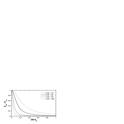
Figure 2: Ratio between the magnetostatic interaction, Eq. (5), and the dipole-dipole interaction, Eq. (10), as a function of $2R/S_{ij}$. Different aspect ratio $L/R$ are considered.

In order to quantify the importance of the interaction energy we calculated the ratio between the self-energy and the magnetostatic interaction energy between two identical nanowires,

$$\eta=\frac{\tilde{E}_{int}(S_{ij})}{2\tilde{E}_{self}}\ .$$ (11)

Figure 3 defines the geometry of the two-wire-system for which $\eta=0.2,$ $0.1,$ $0.01$ and $0.001$. From this figure we observe a strong dependence of the interaction energy on the geometry of the array. As an illustration, when we consider two nanowires with $L=1$ $\mu$m, $R=20$ nm and $L/R=50$, if we look for an almost non interacting regime, $\eta=0.01,2R/S_{ij}=0.068,$ and then the two wires have to be at least $590$ nm apart. For this geometry the interaction energy is about $1\%$ of the self energy. However, for the same $\ L$ and $R$, if the wires are $58$ nm apart ($2R/S_{ij}=0.69$), the interaction energy is about $20\%$ of the self energy ($\eta=0.2)$.

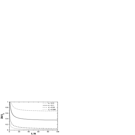
Figure 3: $\eta$ values as a function of the geometry of the two-wire-system.

II.2.2 Wire array

We are now in position to investigate the effect of the interwire magnetostatic coupling in a square array. Calculations for the total interaction energy $\tilde{E}_{int}^{\pm}(N)$ of the $N=n\times n$ square array are shown in Appendix B, and lead us to write

$$\tilde{E}_{array}^{\pm}(n)=2n\sum_{p=1}^{n-1}(n-p)(\pm 1)^{p}\tilde{E}_{int}(pd)\\ +2\sum_{p=1}^{n-1}\sum_{q=1}^{n-1}(n-p)(n-q)(\pm 1)^{p-q}\tilde{E}_{int}(d\sqrt{p^{2}+q^{2}})\ ,$$ (12)

where $+$ ($-$) refers to parallel (antiparallel) magnetic ordering of the nanowires in an array with nearest-neighbor distance $d$, and $\tilde{E}_{int}$ is the interaction energy between two wires given by Eq. (5). Note that in an array $S_{ij}$ is a function of  $d$. In the antiparallel configuration the magnetization of nearest-neighbor nanowires points in opposite directions. Figure 4 illustrates the behavior of $W_{array}^{\pm}(n)=\tilde{E}_{array}^{\pm}(n)/n^{2}$ as a function of $n$ in a ferromagnetic (a) and an antiferromagnetic (b) array. We consider an array of identical wires with $R=20$ nm and $L=1$ $\mu$m and two different nearest-neighbor-distance $d$. We can see that a large number of wires ($N\approx 10^{6}$), corresponding to a sample of $\approx 0.01$ mm², is required for reaching convergence of $W_{array}^{+}(n)$. However, in view of cancellations originated in the different signs of the parallel and antiparallel interactions, the antiparallel configuration converges faster, requiring only the order of 10² wires and a sample of $\approx 1$ $\mu$m².

Figure 4: $W_{array}^{\pm}(n)$ in a square array of identical wires ($R=20$ nm  and $L=1$ $\mu$m). We consider different number of wires in the array and two nearest-neighbor-distances $d$.

We also investigate, for the same wires ($R=20$ nm and $L=1$ $\mu$m), the variation of the asymptotic value of $W_{array}^{\pm}(n)$  as a function of the nearest-neighbor-distance $d$ in a ferromagnetic, (Fig. 5a), and antiferromagnetic array, (Fig. 5b). Figure 5 illustrates our results showing that in the ferromagnetic array, interaction effects decay in an exponential way and extend over long distances as compared with $d.$ Figures 4 and 5 agree with conclusions from experiments by Nielsch et al.Nielsch3 who assume that, due to the high aspect ratio of the magnetic nanowires in an hexagonal array, the stray field interaction extends over several nearest-neighbor-distances.

Figure 5: Asymptotic values of the interaction energy in a square array obtained with $N=10^{6}$ (ferromagnetic array) and $N=10^{2}$ (antiferromagnetic array).

III Concluding Remarks

We have obtained analytical expressions for the magnetostatic interactions between wires. By expanding these expressions we investigate first and second order approximations to the interaction energies showing the range of validity of these expansions. When the wires are apart distances much more larger that their diameter, the first order approximation is valid. We also conclude that the dipole-dipole interaction is valid only when $2R/S_{ij}\simeq 0$. The energy expressions lead us to investigate the extension of the interwire magnetostatic interactions in the array. The number of wires required to reach the convergence in the energy depends on the relative magnetic ordering between nearest-neighbor wires. In the parallel array, a big number of wires is required until convergence. This result implies that the size of the array is an important factor to be consider when different measurements have to be compared.

IV Acknowledgments

This work has been partially supported in Chile by FONDECYT 1050013 and Millennium Science Nucleus “Condensed Matter Physics” P02-054F. CONICYT Ph.D. Fellowship and MECESUP project USA0108 are also acknowledged. One of the authors, J.E., is grateful to the Instituto de Ciencia de Materiales-CSIC for its hospitality.

V Appendix A

In this appendix we calculate the interaction energy of two identical nanowires. We start by replacing the functional form $\mathbf{M}_{i}(\mathbf{r})=M_{0}\sigma_{i}\mathbf{\hat{z}}$ in Eq. (2), leading to

$$E_{int}\left(i,j\right)=\mu_{0}\int\nolimits_{V}M_{iz}\frac{\partial U_{j}}{\partial z}dv\ .$$ (13)

The magnetostatic potential is given by

$$\mathbf{U}(\mathbf{r})=-\frac{1}{4\pi}\int\limits_{V}\frac{\nabla\cdot\mathbf{M}(\mathbf{r}^{\prime})}{\left|\mathbf{r}-\mathbf{r}^{\prime}\right|}\;dv^{\prime}+\frac{1}{4\pi}\int\limits_{S}\frac{\mathbf{\hat{n}}^{\prime}\cdot\mathbf{M}(\mathbf{r}^{\prime})}{\left|\mathbf{r}-\mathbf{r}^{\prime}\right|}\;ds^{\prime}\,,$$

where $V$ and $S$ represent the volume and surface of the wire, respectively.

Due to the functional form of $\mathbf{M}_{i}(\mathbf{r})$, the volumetric contribution to the potential is zero. For the calculation of the surface contribution to the magnetostatic potential, we use the following expansion on the potential Jackson

$$\frac{1}{\left|\mathbf{r}-\mathbf{r}^{\prime}\right|}=\sum_{m=-\infty}^{\infty}e^{im(\phi-\phi^{\prime})}\int\limits_{0}^{\infty}dkJ_{m}(kr_{i})J_{m}(kr^{\prime})e^{-k(z_{>}-z_{<})}\ .$$

Then, the surface contribution to the potential reads Landeros

$$U_{j}=M_{0}\sigma_{j}\sum_{m=-\infty}^{\infty}\int\limits_{0}^{2\pi}d\phi^{\prime}e^{im(\phi-\phi^{\prime})}\int\limits_{0}^{R}r^{\prime}dr^{\prime}\\ \int\limits_{0}^{\infty}dkJ_{m}(kr_{i})J_{m}(kr^{\prime})[e^{-k(L-z)}-e^{-kz}]\ \text{.}$$

After some manipulations, it is straightforward to obtain the potential at a distance $r_{i}$ from the axis of the wire $j$-$th$, $U_{j}$

$$U_{j}=\frac{RM_{0}\sigma_{j}}{2}\int\limits_{0}^{\infty}\frac{dk}{k}J_{1}(kR)J_{0}(kr_{i})[e^{-k(L-z)}-e^{-kz}]\ .$$

Now we need to calculate the dipolar field due to the wire $j$-$th$ experienced by the wire $i$-$th$ a distance $S_{ij}$ apart. In this case

$$r_{i}=\sqrt{r^{2}+S_{ij}^{2}-2rS_{ij}\cos(\phi+\beta)}\ ,$$

where $\beta$ is an arbitrary angle and $r$ defines a particular point in wire $i$. Then, we include in the potential the following expansion Jackson

$$J_{0}\left(k\sqrt{r^{2}+S_{ij}^{2}-2rS_{ij}\cos(\phi+\beta)}\right)\\ =\sum_{m=-\infty}^{\infty}e^{im(\phi+\beta)}J_{m}(kr)J_{m}(kS_{ij})\ ,$$

which lead us to obtain

$$U_{j}=\frac{RM_{0}\sigma_{j}}{2}\int\limits_{0}^{\infty}\frac{dk}{k}J_{1}(kR)[e^{-k(L-z)}-e^{-kz}]\\ \sum_{m=-\infty}^{\infty}e^{im(\phi+\beta)}J_{m}(kr)J_{m}(kS_{ij})\ .$$

By replacing this last expression in Eq. (13) we obtain

$$E_{int}(i,j)=2\mu_{0}M^{2}\sigma_{i}\sigma_{j}\pi R^{2}\\ \int\limits_{0}^{\infty}\frac{dk}{k^{2}}J_{1}^{2}(kR)J_{0}(kS_{ij})(1-e^{-kL})\ .$$

Finally, and changing the variable $q=kL$, we obtain the reduced expression presented in the Eq. (5),

$$\tilde{E}_{int}(i,j)=2\sigma_{i}\sigma_{j}\int\limits_{0}^{\infty}\frac{dq}{q^{2}}J_{1}^{2}\left(\frac{qR}{L}\right)J_{0}\left(\frac{qS_{ij}}{L}\right)(1-e^{-q})\ .$$

VI Appendix B

The total interaction energy of the $N=n\times n$ square array can be written as

$$\tilde{E}_{array}^{\pm}(n)=\frac{1}{2}\sum_{i=1}^{n}\sum_{j=1}^{n}\sum_{k=1}^{n}\sum_{l=1}^{n}(\pm 1)^{(k-i)-(l-j)}\\ \tilde{E}_{int}\left(d\sqrt{(k-i)^{2}+(l-j)^{2}}\right)\ ,$$

where $+$ ($-$) refers to parallel (antiparallel) nearest-neighbor magnetic orientation of the nanowires in the array. Here $\tilde{E}_{int}\left(0\right)=0$, avoiding the self-interaction of the wires. For simplicity we define the following function

$$f^{\pm}(p,q)=(\pm 1)^{p-q}\tilde{E}_{int}(d\sqrt{p^{2}+q^{2}})\ ,$$ (14)

which can be used to write the interaction energy in a compact form; that is

$$\tilde{E}_{array}^{\pm}(n)=\frac{1}{2}\sum_{i=1}^{n}\sum_{j=1}^{n}\sum_{k=1}^{n}\sum_{l=1}^{n}f^{\pm}(k-i,l-j)\ .$$ (15)

We can reduce the number of summations using the following rule

$$\sum_{i=1}^{n}\sum_{k=1}^{n}g(k-i)=ng(0)+\sum_{p=1}^{n-1}(n-p)[g(p)+g(-p)]\ ,$$ (16)

which lead us to write

$$\sum_{i=1}^{n}\sum_{k=1}^{n}f^{\pm}(k-i,l-j)=nf^{\pm}(0,l-j)\\ +2\sum_{p=1}^{n-1}(n-p)f^{\pm}(p,l-j)\ .$$

Then, the interaction energy, Eq. (15), reduces to

$$\tilde{E}_{array}^{\pm}(n)=\frac{n}{2}\sum_{j=1}^{n}\sum_{l=1}^{n}f^{\pm}(0,l-j)\\ +\sum_{p=1}^{n-1}(n-p)\sum_{j=1}^{n}\sum_{l=1}^{n}f^{\pm}(p,l-j)\ .$$ (17)

Using again the rule (16), we can reduce the double-sums in Eq. (17), obtaining

$$\tilde{E}_{int}^{\pm}(n)=\frac{n^{2}}{2}f^{\pm}(0,0)+n\sum_{q=1}^{n-1}(n-q)f^{\pm}(0,q)\\ +n\sum_{p=1}^{n-1}(n-p)f^{\pm}(p,0)+2\sum_{p=1}^{n-1}\sum_{q=1}^{n-1}(n-p)(n-q)f^{\pm}(p,q)\ .$$

From (14) we know that $f^{\pm}(0,0)\equiv 0$, which lead us to finally obtain

$$\tilde{E}_{array}^{\pm}(n)=2n\sum_{p=1}^{n-1}(n-p)(\pm 1)^{p}\tilde{E}_{int}\left(pd\right)\\ +2\sum_{p=1}^{n-1}\sum_{q=1}^{n-1}(n-p)(n-q)(\pm 1)^{p-q}\tilde{E}_{int}\left(d\sqrt{p^{2}+q^{2}}\right)\ .$$

References

- (1) G. Prinz, Science 282, 1660 (1998).
- (2) R. P. Cowburn and M. E. Welland, Science 287, 1466 (2000).
- (3) P. O. Jubert and R. Allenspach, Phys. Rev. B 70, 144402 (2004).
- (4) F. Porrati and M. Huth, Appl. Phys. Lett. 85, 3157 (2004).
- (5) P. Landeros, J. Escrig, D. Altbir, D. Laroze, J. d’Albuquerque e Castro and P. Vargas, Phys. Rev. B 71, 094435 (2005).
- (6) J. Escrig, P. Landeros, D. Altbir, M. Bahiana and J. d’Albuquerque e Castro, Appl. Phys. Lett. 89, 132501 (2006).
- (7) K. Nielsch, R. B. Wehrspohn, J. Barthel, J. Kirschner, S. F. Fischer, H. Kronmuller, T. Schweinbock, D. Weiss and U. Gosele, J. Magn. Magn. Mater. 291, 234-240 (2002).
- (8) K. Nielsch, R. B. Wehrspohn, J. Barthel, J. Kirschner, U. Gosele, S. F. Fischer and H. Kronmuller, Appl. Phys. Lett. 79, 1360 (2001).
- (9) M. Vázquez, K. Nielsch, P. Vargas, J. Velázquez, D. Navas, K. Pirota, M. Hernández-Vélez, E. Vogel, J. Cartes, R. B. Wehrspohn and U. Gosele, Physica B 343, 395 (2004).
- (10) M. Vázquez, K. Pirota, J. Torrejón, D. Navas and M. Hernández-Vélez, J. Magn. Magn. Mater. 294, 174 (2005).
- (11) J. I. Martín, J. Nogués, K. Liu, J. L. Vicent and I. K. Schuller, J. Magn. Magn. Mater. 256, 449 (2003)
- (12) C. Ross, Ann. Rev. Mater. Res. 31, 203 (2001).
- (13) R. Skomski, H. Zeng, M. Zheng and D. J. Sellmyer, Phys. Rev. B 62, 3900 (2000).
- (14) R. Varga, K. L. Garcia, M. Vázquez and P. Vojtanik, Phys. Rev. Lett. 94, 017201 (2005).
- (15) L. C. Sampaio, E. H. C. P. Sinnecker, G. R. C. Cernicchiaro, M. Knobel, M. Vázquez and J. Velázquez, Phys. Rev. B 61, 8976 (2000).
- (16) M. Knobel, L. C. Sampaio, E. H. C. P. Sinnecker, P. Vargas and D. Altbir, J. Magn. Magn. Mater. 249, 60 (2002).
- (17) J. Velázquez and M. Vázquez, J. Magn. Magn. Mater. 249, 89-94 (2002).
- (18) J. Velázquez and M. Vázquez, Physica B 320, 230-235 (2002).
- (19) Qing-Feng Zhan, Jian-Hua Gao, Ya-Qiong Liang, Na-Li Di and Zhao-Hua Cheng, Phys. Rev. B 72, 024428 (2005).
- (20) J. Velázquez, K. R. Pirota and M. Vázquez, IEEE Trans. Magn. 39, 3049 (2003).
- (21) R. Hertel, J. Appl. Phys. 90, 5752 (2001).
- (22) L. Clime, P. Ciureanu and A. Yelon, J. Magn. Magn. Mater. 297, 60 (2006).
- (23) M. Bahiana, F. S. Amaral, S. Allende and D. Altbir, Phys. Rev. B 74, 174412 (2006).
- (24) A. Aharoni, Introduction to the Theory of Ferromagnetism (Clarendon Press, Oxford, 1996).
- (25) J. D. Jackson, Classical electrodynamic, 2nd edition (John Wiley & Sons, Inc., USA, 1975).