Valley Kondo Effect in Silicon Quantum Dots

Abstract

Recent progress in the fabrication of quantum dots using silicon opens the prospect of observing the Kondo effect associated with the valley degree of freedom. We compute the dot density of states using an Anderson model with infinite Coulomb interaction $U$, whose structure mimics the nonlinear conductance through a dot. The density of states is obtained as a function of temperature and applied magnetic field in the Kondo regime using an equation-of-motion approach. We show that there is a very complex peak structure near the Fermi energy, with several signatures that distinguish this spin-valley Kondo effect from the usual spin Kondo effect seen in GaAs dots. We also show that the valley index is generally not conserved when electrons tunnel into a silicon dot, though the extent of this non-conservation is expected to be sample-dependent. We identify features of the conductance that should enable experimenters to understand the interplay of Zeeman splitting and valley splitting, as well as the dependence of tunneling on the valley degree of freedom.

I I. Introduction

Experimentation on gated quantum dots (QDs) has generally used GaAs as the starting material, due to its relative ease of fabrication. However, the spin properties of dots are becoming increasingly important, largely because of possible applications to quantum information and quantum computing. Since the spin relaxation times in GaAs are relatively short, Si dots, with much longer relaxation times Jantsch2002 ; Tyryshkin2005 ; Tyryshkin2003 ; DasSarma2003 , are of great scientific and technological interest Eriksson2004 . Recent work has shown that few-electron laterally gated dots can be made using Si Jones2006 Klein2004 , and single-electron QDs are certainly not far away.

There is one important qualitative difference in the energy level structures of Si and GaAs: the conduction band minimum is two-fold degenerate in the strained Si used for QDs as compared to the non-degenerate minimum in GaAs. Thus each orbital level has a fourfold degeneracy including spin. This additional multiplicity is referred to as the valley degeneracy. For applications, this degeneracy poses challenges - it must be understood and controlled. From a pure scientific viewpoint, it provides opportunities - the breaking of the degeneracy is still poorly understood.

Previous experimental work has shown that in zero applied magnetic field the splitting of the degeneracy is about $1.5\pm 0.6$ $\mu$eV in two-dimensional electron gases (2DEGs) srijit_nature and that it increases when the electrons are further confined in the plane srijit_nature . Surprisingly, the splitting increases linearly with applied field. Theoretical understanding of these results has historically been rather poor, with theoretical values much larger than experimental ones for the zero-field splittings TBBoykin2004_2 TBBoykin2004 and theory also predicting a nonlinear field dependence Ohkawa1977 . Recent work indicates that consideration of surface roughness may resolve these discrepancies Friesen2006 . In Si QDs, a related issue is also of importance: what is the effect of valley degeneracy on the coupling of the leads to the dots? The spin index is usually assumed to be conserved in tunneling. Is the same true of the valley index?

Recent measurements of the valley splitting in a quantum point contact show a valley splitting much larger than in the 2DEGs, about $1$ meV in  quantum point contacts srijit_nature . A QD in a similar potential well is expected to produce a valley splitting of the same order of magnitude. The overall picture of the degeneracy is as shown in Fig. 1 for a single orbital level of a Si QD. Of particular interest is the fact that a level crossing must occur, and the rough value of the applied field at this point is $B_{cr}\approx 2.5$ T, given a reasonable zero-field valley splitting of $0.5$ meV, and the valley-spin slope of magnetic field for the $"o\uparrow"$ state to be $0.1$ meV/T, as it is in Hall bars.

The aim of this paper is to study the Kondo effect in the context of transport through a Si dot. The Kondo effect was originally discovered in dilute magnetic alloys. At low temperatures, the electron in a single impurity forms a spin singlet with electrons in the conduction band, thus causing an increasing resistance as the temperature is reduced to zero. Since the first observations of the Kondo effect in GaAs QDs, there has been considerable experimental and theoretical work done, mainly because QDs provide an excellent playground where one can tune physical parameters such as the difference between energy levels in QDs and the Fermi level, the coupling to the leads, and the applied voltage difference between the leads. The level of scientific understanding of this purely spin Kondo effect in QDs is on the whole quite satisfactory. The basic phenomena are as follows. At temperature $T\leq T_{K}$, where the Kondo effect appears, a zero-bias peak in the dot conductance is observed. An applied magnetic field splits the peak into two peaks separated by twice the Zeeman energy $2g\mu_{B}B$.  These linear peak energy dependencies on the applied magnetic field have been observed in GaAs QDs Goldhaber1998 . The Kondo effect only occurs when the occupation of the dot is odd.

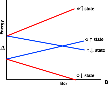
Figure 1: Schematic diagram of the energy levels of a single orbital in a Si QD in a magnetic field.  The quantum numbers are even ($e$), odd ($o$) valley states and up and down spin projections for spin $1/2$ states. A level crossing occurs at the magnetic field $B_{cr}$.

Clearly, Si dots will have a much richer phenomenology. There are multiple field dependencies as seen in Fig. 1, and the additional degeneracy can give rise to several Kondo peaks even in zero field. Furthermore, the Kondo temperature is enhanced when the degeneracy is increased. We build on previous work on the orbital Kondo effect. For example, an enhanced Kondo effect has been observed due to extra orbital degree of freedom in carbon nanotubes (CNTs) Jarillo Choi2005 and in a vertical QD, with magnetic field-induced orbital degeneracy for an odd number of electrons and spin 1/2 Sasaki . More complex peak structure in their differential conductance suggests entangled interplay between spin and orbital degrees of freedom.  We also note that a zero-bias peak has been observed in Si MOSFET structures tsui .

Our goal will be to elucidate the characteristic structures in the conductance, particularly their physical origin, and their temperature and field dependencies. Once this is done, one can hope to use the Kondo effect to understand some of the interesting physics of Si QDs, particularly the dependence of tunneling matrix elements on the valley degree of freedom.

This paper is organized as follows. In Sec.II, we determine whether valley index conservation is to expected; in Sec. III, we introduce our formalism; in Sec. IV, we discuss the effect of valley index non-conservation; in Sec. V, we present our main results; in Sec. VI we summarize the implications for experiments.

II II. Tunneling with valley degeneracy

The basic issue at hand is the conductance of a dot with valley degeneracy, and the influence of the Kondo effect on this process.  The dots we have in mind are separated electrostatically from 2DEG leads on either side.  These 2DEGs have the same degeneracy structure.  Thus before we tackle the issue of the conductance we need the answer to a preliminary question: is the valley index conserved during the tunneling process from leads to dots?  Non-conservation of the valley index will introduce additional terms in the many-body Hamiltonian that describes the dots, and, as we shall see below, it changes the results for the conductance.  In this section, we investigate the question of valley index conservation in a microscopic model of the leads and dots.  We do this in the context of a single-particle problem that should be sufficient to understand the parameters of the many-body Hamiltonian that will be introduced in Sec. III.

If we have a system consisting of leads and a QD in a 2DEG of strained Si, then both the leads and the dot will have even and odd valley states if the interfaces defining the 2DEG are completely smooth.  The valley state degeneracy is split by a small energy. If the valley index is conserved during tunneling, then the even valley state in the lead will only tunnel into the even valley state in the dot. On the other hand, if the valley index is not conserved, then the even valley state in the lead will tunnel into both the even and odd valley states in the dot; similarly for the odd valley state in the lead. We can estimate the strength of the couplings between the various states in the leads and the dot by calculating the hopping matrix elements between them.

Consider a system of a lead and a dot in a SiGe/Si/SiGe quantum well, separated by a barrier of height $V_{b}$. If $V_{b}=\infty$, there will be no tunneling between the lead and the dot and the eigenstates of the whole system can be divided into lead states $|\Psi_{L,(e,o)}^{\infty}\rangle$ and dot states $|\Psi_{D,(e,o)}^{\infty}\rangle$ where $e,~{}o$ are the even and the odd valley states. Call the Hamiltonian for this case $H_{0}$. When $V_{b}$ is lowered to a finite value, there will be some amount of tunneling of the lead wavefunction into the dot. Call the Hamiltonian for this case $H$. This can be thought of as a perturbation problem where the $n^{th}$ perturbed eigenstate $|n\rangle$ is no longer the $n^{th}$ unperturbed eigenstate $|n^{0}\rangle$ but acquires components along the other unperturbed eigenstates $|k^{0}\rangle$. The perturbation Hamiltonian is $H^{\prime}=H-H_{0}.$  $H^{\prime}$ considered as a function of position is not small, but the matrix elements of  $H^{\prime}$ are small. This means that in the $1^{st}$ order perturbation theory we can write the perturbed $n^{th}$ state as

$$|n\rangle=|n^{0}\rangle+\sum_{k\neq n}|k^{0}\rangle\frac{V_{kn}}{E_{n}^{0}-E_{k}^{0}}$$ (1)

where $V_{kn}=\langle k^{0}|H^{\prime}|n^{0}\rangle$ is the hopping or tunneling matrix term.

If we further assume that the tunneling Hamiltonain conserves spin and that only one orbital state need be considered on the QD, we can expand the perturbed even valley lead wavefunction (with tunneling) as

$$|\Psi_{L,e}\rangle=|\Psi_{L,e}^{\infty}\rangle+\frac{V_{e,e}}{|E_{Le}^{0}-E_{De}^{0}|}|\Psi_{D,e}^{\infty}\rangle+\frac{V_{e,o}}{|E_{Le}^{0}-E_{Do}^{0}|}|\Psi_{D,o}^{\infty}\rangle$$ (2)

Usually, in a perturbation problem, the unperturbed wavefunctions and the hopping matrix elements are known and used to find the perturbed wavefunction. However in the present case we use a model to compute the perturbed and unpertubed wavefunctions and use these to determine the unknown hopping matrix elements $V_{e,e}$ $V_{e,o}.$  These will be needed in later sections.

From the above equation,

$$V_{e,e} = (|E_{Le}^{0}-E_{De}^{0}|)\langle\Psi^{\infty}_{De}|\Psi_{Le}\rangle$$ (3)

$$V_{e,o} = (|E_{Le}^{0}-E_{Do}^{0}|)\langle\Psi^{\infty}_{Do}|\Psi_{Le}\rangle$$ (4)

The perturbed and the unperturbed wavefunctions and the corresponding energies are calculated by using an empirical 2D tight binding model with nearest ($v_{z}$) and next nearest neighbor interactions ($u_{z}$) along the $z$ (growth) direction and the nearest neighbor interactions ($v_{x}$) along the $x$ direction (in the plane of the 2DEG). Potential barriers and edges of the quantum well are modeled by adjusting the onsite parameter ($\epsilon$) on the atoms. This is an extension of the 2-band 1D tight binding model outlined by Boykin et al. TBBoykin2004_2 ; TBBoykin2004 , considering only the lowest conduction band of Si. This is a single particle calculation with the magnetic field $B=0$. Note that the parameters from the Boykin et al. model are chosen precisely so as to reproduce the two-valley structure of strained Si.

The single-particle Hamiltonian for the system is

$$H = \sum_{x}~{}[~{}\epsilon|\phi(x,z)\rangle\langle\phi(x,z)|+v_{x}|\phi(x,z)\rangle\langle\phi(x+1,z)|+v_{z}|\phi(x,z)\rangle\langle\phi(x,z+1)|$$ (5)

$$+ u_{z}|\phi(x,z)\rangle\langle\phi(x,z+2)|+v_{x}|\phi(x-1,z)\rangle\langle\phi(x,z)|+v_{z}|\phi(x,z-1)\rangle\langle\phi(x,z)|$$

$$+ u_{z}|\phi(x,z-2)\rangle\langle\phi(x,z)|~{}]$$

The parameters defining the system are as follows: the lead is $80$ atoms long, the barrier between the lead and the dot is $16$ atoms wide along $x$ and $0.3$ eV high, the QD is $38$ atoms ($\approx 10~{}$nm) wide along $x$ and $38$ atoms wide along $z$, the barrier along $z$ defining the quantum well is $20$ atoms wide on each side and its height is $0.3$ eV. The nearest and next nearest neighbor interaction terms along $z$ are $v_{z}=0.68264$ eV, and $u_{z}=0.611705$ eV, and that along $x$ is $v_{x}=-10.91$ eV.  The schematic of the system is shown in Fig. 2

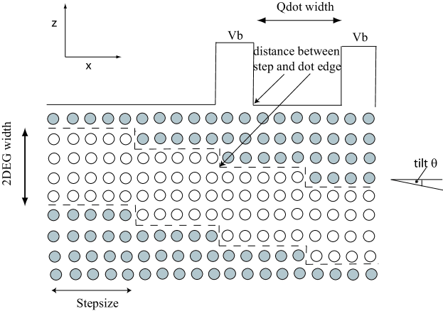
Figure 2: The system of the lead and the dot in a miscut quantum well with the potential profile along the $x$-direction. The open circles represent Si atoms sandwiched between the SiGe atoms in the barrier region represented by the filled circles.

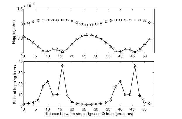
Figure 3: (a)Tunneling matrix elements ($V_{e,e},V_{e,o}$) in units of eV and (b) Ratio of the tunneling matrix elements ($V_{e,o}/V_{e,e}$) as a function of the relative distance between the step edge and the quantum dot edge for constant barrier height and width (for a miscut QW). The solid line with triangular markers indicate the $V_{e,e}$ term and the dashed line with open circles indicate the $V_{e,o}$ term. Here the stepsize is constant at $30$ atoms ($\approx 2^{o}$ tilt)

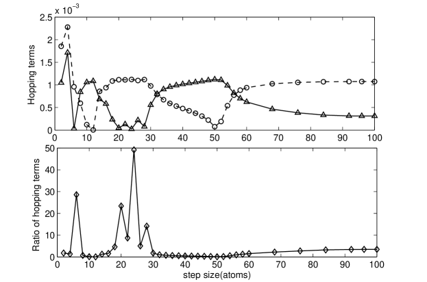
Figure 4: (a)Tunneling matrix elements ($V_{e,e},V_{e,o}$) in units of eV and (b) Ratio of the tunneling matrix elements ($V_{e,o}/V_{e,e}$) as a function of the stepsize for constant barrier height and width (for a miscut QW). The solid line with triangular markers indicate the $V_{e,e}$ term and the dashed line with open circles indicate the $V_{e,o}$ term. Here the step edge coincides with the quantum dot edge.

We consider two kinds of 2DEGs, one with no interface roughness at the interface and the other with a miscut of about $2^{\circ}$. We find that the valley index is conserved in the case of smooth interfaces. We model the miscut interface as a series of regular steps of one atom thickness and width defined by the tilt, $e.g.,$ a $2^{\circ}$ tilt corresponds to a step length of about $30$ Si atoms. In this case, the valley index is no longer conserved. Strengths of the coupling between the $e-e$ and $e-o$ valley states is found to depend strongly on the relative distance between the edge of the closest step and the edge of the quantum dot. In Fig. 3, we plot the hopping matrix elements as a function of this relative distance. The terms show oscillations that have a period equal to the step size in this case.

The coupling strengths are also found to depend on the tilt of the substrate on which the 2DEG is grown. We show in Fig. 4, the hopping matrix elements as a function of the stepsize ($\propto$ 1/ tilt) and find that the hopping terms vary rapidly at small step sizes ($i.e$ large tilts) but slowly at larger stepsizes ($i.e.,$ smaller tilts).

In a quantum well, the phases of the rapid oscillations of the electron wavefunctions (along the z-direction) are locked to the interface and in a well with smooth interfaces, the phase remains the same for a particular valley throughout friesen1 . But in a miscut well, the phases are different for electrons localized at different steps even for the same valley eigenstate. The resultant valley splitting is due to interference of phase contributions from all the steps. Hence the valley splitting can be very different in the lead and the dot. The same argument explains the conservation of the valley index across the barrier in the lead-dot system. In the case of a smooth interface, the $e$ eigenstate in the lead has same phase of the z-oscillations as the $e$ eigenstate in the dot, and is $90^{\circ}$ out of phase with the $o$ eigenstate in the dot. Hence, there is a finite overlap between the $e-e$ wavefunctions, while the $e-o$ overlap cancels out due to interference. This preserves the valley index during the tunneling.

In the case of a miscut well, we can no longer strictly label the eigenstates $e$ or $o$, but let us continue to do so just for convenience. Here, because $e$ in the lead does not really have a single phase along $z$ but is composed of different phases at each step and similarly for $o$ in the dot, there is a fair chance that there will be a non-cancellation of the phases between the $e,~{}o$ wavefunctions depending up the the extent of tunneling. This will give rise to a finite hopping matrix term between all the dot and lead states and the valley index $o,~{}e$ can longer be said to be conserved.

The results show that the conservation or non-conservation of the valley index depends sensitively on fine details of the dot morphology such the proximity of a step edge to the edge of the dot on atomic scales.  It is not likely that good control at this level can be achieved, and thus some sample dependence must be expected.  This means that it will normally be necessary to include hopping terms that do not conserve valley index into the Hamiltonian in order to understand the Kondo effect in realistic Si QDs, where the interfaces are rarely smooth.

III III. Equation-of-Motion Approach in the $U\rightarrow\infty$ limit

Sec. II has given us some insight into the nature of the tunneling between the leads and the dot.  We now introduce a Hamiltonian to describe the full many-body problem, and discuss the computational method we will use to solve it.  This Hamiltonian must include the single-particle energy levels of the leads and the dot, the tunneling matrix elements that connect these levels, and the Coulomb interaction between electrons on the dot.  We shall use the Anderson impurity model:

$$\mathcal{H} = \sum_{ikm\sigma}\varepsilon_{k}c_{ikm\sigma}^{+}c_{ikm\sigma}+\sum_{m\sigma}\varepsilon_{m\sigma}f_{m\sigma}^{+}f_{m\sigma}+\sum_{ikm\sigma}V_{0,ik}(c_{ikm\sigma}^{+}f_{m\sigma}+f_{m\sigma}^{+}c_{ikm\sigma})$$

$$+\sum_{ikm\sigma}V_{X,ik}(c_{ikm\sigma}^{+}f_{\bar{m}\sigma}+f_{\bar{m}\sigma}^{+}c_{ikm\sigma})+\frac{U}{2}\sum_{m^{\prime}\sigma^{\prime}\not=m\sigma}n_{m^{\prime}\sigma^{\prime}}n_{m\sigma}$$

Here $\sigma$ indicate two-fold spin $1/2$ and $m$ two-fold valley indices. $\bar{m}$ means the opposite valley state of $m$. The operator $c_{ikm\sigma}^{+}(c_{ikm\sigma})$ creates (annihilates) an electron with an energy $\varepsilon_{k}$ in the $i$ lead, $i\in L,R$, while the operator $f_{m\sigma}^{+}(f_{m\sigma})$ creates (annihilates) an electron with an energy $\varepsilon_{m\sigma}$ in the QD, connected to the leads by Hamiltonian couplings $V_{0,ik}$ and $V_{X,ik}$ which correspond to an electron tunneling between the same valley states and different valley states, respectively. We assume that the $V_{0(X),ik}$ do not depend on spin index $\sigma$. $U$ is the Coulomb interaction on the dot.  It is assumed to be independent of $m.$  Previous studies on the orbital Kondo effect have mostly assumed conservation of orbital indices orbitkondo .  Recent theoretical work has found that a transition occurs from $SU(4)$ to $SU(2)$ Kondo effect by allowing violation of conservation of orbital index in CNTs Choi2005 ; JSLim2006 or in double QDs Chudnovskiy2005 . For Si QDs, we have shown from the previous section that tunnelings between different valley states have to be taken into account.

Experiments measure the current $I$ as a function of source-drain voltage $V_{sd}.$  The differential conductance $G=d\mathrm{I}/d\mathrm{V}_{sd}$ is given by the generalized Landauer formula Landauer

$$\mathrm{I}=\frac{e}{h}\sum_{m\sigma}\int_{-D}^{D}dw(f_{L}(w)-f_{R}(w))\frac{2\Gamma_{L,m\sigma}(w)\Gamma_{R,m\sigma}(w)}{\Gamma_{L,m\sigma}(w)+\Gamma_{R,m\sigma}(w)}\mathrm{Im}[\mathcal{G}_{m\sigma}(w)]$$

where $D$ is the bandwidth and $\Gamma_{i,m\sigma}(w)=2\pi\sum_{k}(V_{0,ik}^{2}+V_{X,ik}^{2})\delta(w-\varepsilon_{k})$. The $f^{\prime}s$ are Fermi functions calculated with chemical potentials $\mu_{L}$ and $\mu_{R}$ with $\mu_{L}=\mu_{R}+e\mathrm{V}_{sd}.$  In the following argument, we assume a flat unperturbed density of states and $V_{0,ik}=V_{0},~{}V_{X,ik}=V_{X}$. We then define $\Gamma=\Gamma_{L,m\sigma}(w)+\Gamma_{R,m\sigma}(w)=\pi V^{2}/D$ with $V^{2}=V_{0}^{2}+V_{X}^{2}$.   With these approximations we may differentiate this equation and we find $d\mathrm{I}/d\mathrm{V}_{sd}\sim$ $-\mathrm{Im}[\mathcal{G}_{m\sigma}(e\mathrm{V}_{sd})]/\pi=$ density of states(DOS).  Here $\mathcal{G}_{m\sigma}(w)$ is the retarded Green’s function:

$$\mathcal{G}_{m\sigma}(w)=\ll f_{m\sigma},f_{m\sigma}^{+}\gg=-i\int_{0}^{\infty}e^{i\alpha t}<\{f_{m\sigma}(t),f_{m\sigma}^{+}(0)\}>dt.$$ (6)

where $\alpha=w+i\delta$. Here $\{,\}$ and $<,>$ denote the anti-commutator and statistical average of operators, respectively.  Hence our task is to compute $\mathcal{G}_{m\sigma}(w).$  Although the approximation of a flat density of states is not likely to be completely valid, we still expect that sharp structures in $\mathcal{G}_{m\sigma}(w)$ will be reflected in the voltage dependence of $d\mathrm{I}/d\mathrm{V}_{sd}\mathrm{.}$

Several approximate solution methods for this type of Hamiltonian have been used successfully: numerical renormalization group, non-crossing approximation(NCA), scaling theory, and equation-of-motion (EOM) approach. In this paper, we use the EOM approach to investigate the transport through a Si QD at low temperature, in the presence of magnetic field. The EOM approach has several merits. The most important for our purposes is that it can produce the Green’s function at finite temperature, and works both for infinite-$U$ and finite-$U$. We basically follow the spirit of the paper by Czycholl Czycholl which gives a thorough analysis of EOM in the large-$N$ limit($N$ is the number of energy level degeneracy) and provides a suitable approximation for finite-$U$ systems. Though in the present case $N$ is $4$, the Green’s function obtained from EOM should give a reasonable picture in the case of a weak hybridization and relatively large $U$.  The approximation starts from the equations of motion for $\mathcal{G}_{m\sigma}(w)$ in the frequency domain:

$$w\ll A,B\gg=<\{A,B\}>+\ll[A,H],B\gg=<\{A,B\}>+\ll A,[H,B]\gg.$$

This can be obtained by integrating Eq. 6 by parts. The detailed derivation for the Green’s function $\mathcal{G}_{m\sigma}$ is given in the Appendix. We truncate higher-order Green’s functions by using a scheme adopted by Lacroix1981 ; Luo2002 ; Kashcheyevs2006 . The higher-order Green’s functions are of the general forms $\ll f^{+}cc,f^{+}\gg$ and $\ll fc^{+}c,f^{+}\gg$ (we drop indices for the sake of generalization) which we decouple by replacing them with

$$\ll f^{+}cc,f^{+}\gg = <f^{+}c>\ll c,f^{+}\gg$$

$$\ll fc^{+}c,f^{+}\gg = <c^{+}c>\ll f,f^{+}\gg.$$

We combine Eq. A.1, A.2, A.17, and A.18 and take the limit $U\rightarrow\infty$. We obtain coupled Green’s functions expressed by

$$R(z)\mathcal{G}_{m\sigma} = 1-\sum_{l\not=m\sigma}<n_{l}>-\sum_{l\not=m\sigma}\tilde{A}_{l}(z)+P(z)\mathcal{M}_{\bar{m}\sigma}$$

$$\bar{R}(\bar{z})\mathcal{M}_{\bar{m}\sigma} = <f_{m\sigma}^{+}f_{\bar{m}\sigma}>+\widetilde{\bar{F}}_{m\sigma}(w)+\bar{P}(\bar{z})\mathcal{G}_{m\sigma},$$ (7)

where $\mathcal{M}_{\bar{m}\sigma}\equiv\ll f_{\bar{m}\sigma},f_{m\sigma}^{+}\gg$ is the correlation function between different valley states. We denote $z=w-\varepsilon_{m\sigma}+\varepsilon_{l\not=m\sigma}$ and $\bar{z}=w-\varepsilon_{\bar{m}\sigma}+\varepsilon_{p\not=\bar{m}\sigma}$. The propagators $R(z),~{}\bar{R}(\bar{z})$ and $~{}P(z)$, $\bar{P}(\bar{z})$ are defined as follows

$$R(z) = w-\varepsilon_{m\sigma}-\Sigma_{a}(w)(1-\sum_{l\not=m\sigma}\tilde{A}_{l}(z))-\sum_{l\not=m\sigma}\Sigma_{c,l}(z)-\Sigma_{b}(w)\widetilde{F}_{m\sigma}(w)-\sum_{l\not=m\sigma}\widetilde{J}_{l}(z)$$

$$\bar{R}(\bar{z}) = w-\varepsilon_{\bar{m}\sigma}-\Sigma_{a}(w)(1-\sum_{p\not=\bar{m}\sigma}\tilde{A}_{p}(\bar{z}))-\sum_{p\not=\bar{m}\sigma}\Sigma_{c,p}(\bar{z})-\Sigma_{b}(w)\widetilde{\bar{F}}_{m\sigma}(w)-\sum_{p\not=\bar{m}\sigma}\widetilde{J}_{p}(\bar{z})$$

$$P(z) = \Sigma_{b}(w)(1-\sum_{l\not=m\sigma}\tilde{A}_{l}(z))-\Sigma_{d}(w)-\tilde{I}_{m\sigma}(w)+\Sigma_{a}(w)\widetilde{F}_{m\sigma}(w)$$

$$\bar{P}(\bar{z}) = \Sigma_{b}(w)(1-\sum_{p\not=\bar{m}\sigma}\tilde{A}_{p}(\bar{z}))-\Sigma_{d}(w)-\tilde{\bar{I}}_{m\sigma}(w)+\Sigma_{a}(w)\widetilde{\bar{F}}_{m\sigma}(w).$$

Note that $l\not=m\sigma,~{}p\not=\bar{m}\sigma$. The various functions in $R(z),~{}\bar{R}(\bar{z}),~{}P(z)$, and $\bar{P}(\bar{z})$ are defined in Eq. A.19-A.28 in the Appendix. Moreover, they can be self-consistently computed. We proceed to solve for $\mathcal{G}_{m\sigma}$ and $\mathcal{M}_{\bar{m}\sigma}$

$$\mathcal{G}_{m\sigma} = \frac{1-\sum_{l\not=m\sigma}<n_{l}>-\sum_{l\not=m\sigma}\tilde{A}_{l}(z)+(<f_{m\sigma}^{+}f_{\bar{m}\sigma}>+\widetilde{\bar{F}}_{m\sigma}(w))P(z)/\bar{R}(\bar{z})}{R(z)-P(z)\bar{P}(\bar{z})/\bar{R}(\bar{z})}$$ (8)

$$\mathcal{M}_{\bar{m}\sigma} = \frac{<f_{m\sigma}^{+}f_{\bar{m}\sigma}>+\widetilde{\bar{F}}_{m\sigma}(w)+(l-\sum_{l\not=m\sigma}<n_{l}>-\sum_{l\not=m\sigma}\tilde{A}_{l}(z))\bar{P}(\bar{z})/R(z)}{\bar{R}(\bar{z})-\bar{P}(\bar{z})P(z)/R(z)}.$$ (9)

$P(z),~{}\bar{P}(\bar{z})$ express the correlations between $"m\sigma"$ and $"\bar{m}\sigma"$ states. If $V_{X}=0$, then $P(z)=0$, Coupled Eqs. 7 are decoupled and reduced to the Green’s function with conserved valley index. Furthermore, when $V_{X}\not=0$, peak structure will alter since the function $\Sigma_{d}(w)$ in $P(z),~{}\bar{P}(\bar{z})$ has a second-order logarithmic divergence at the Fermi level. Now we have a set of self-consistent equations for $\mathcal{G}_{m\sigma}$ from Eq. 8, since $\tilde{A}_{m\sigma}(z)$, $<n_{m\sigma}>,~{}<f_{m\sigma}^{+}f_{\bar{m}\sigma}>$ and other terms such as $\tilde{I}_{m\sigma}(w),~{}\tilde{F}_{m\sigma}(w),~{}\tilde{J}_{m\sigma}(z)$ are integrals over $\mathcal{G}_{m\sigma}$ and $\mathcal{M}_{\bar{m}\sigma}$ themselves. We solve by taking an initial guess for $\mathcal{G}_{m\sigma}$ and $\mathcal{M}_{\bar{m}\sigma}$ of the forms

$$\mathcal{G}_{m\sigma}^{0}(w) = \frac{1-\sum_{l\not=m\sigma}<n_{l}>}{w-\varepsilon_{m\sigma}+iN\Gamma\pi}.$$

$$\mathcal{M}_{\bar{m}\sigma}^{0}(w) = \frac{<f_{m\sigma}^{+}f_{\bar{m}\sigma}>}{w-\varepsilon_{\bar{m}\sigma}+iN\Gamma\pi}.$$

These have the expected structure of a broad peak of width $N\Gamma$ $(N=4)$ centered around the energy $\varepsilon_{m\sigma}$ for $\mathcal{G}_{m\sigma}$ and $\varepsilon_{\bar{m}\sigma}$ for $\mathcal{M}_{\bar{m}\sigma}$, and the narrow Kondo peak(s) around the Fermi level.   We then iterate to self-consistency, at each stage determining the occupation numbers $<n_{m\sigma}>$ and expectation values $<f_{m\sigma}^{+}f_{\bar{m}\sigma}>$ fromfoot_note1

$$<n_{m\sigma}> = -\frac{1}{\pi}\int dwf_{FD}(w)\mathrm{Im}\mathcal{G}_{m\sigma}.$$

$$<f_{m\sigma}^{+}f_{\bar{m}\sigma}> = -\frac{1}{\pi}\int dwf_{FD}(w)\mathrm{Im}\mathcal{M}_{\bar{m}\sigma}.$$

Here $f_{FD}$ is the Fermi function.

IV IV. Effects of non-conservation of valley index

Consider all four-fold valley and spin levels to be degenerate, meaning no magnetic field and no zero-field valley splitting. We have $R(z)=\bar{R}(\bar{z})$, $P(z)=\bar{P}(\bar{z})$ and $z=\bar{z}=w$. We define the Kondo temperature as the temperature at which the real part of the denominator of the Green’s function vanishes. As discussed by Hewson Hewson , this definition gives the temperature that controls the thermodynamics.  We rewrite Eq. 8 in order to explicitly express two contributions from $\mathcal{G}_{m\sigma}$,

$$\mathcal{G}_{m\sigma} = \frac{1-\sum_{l\not=m\sigma}<n_{l}>-\sum_{l\not=m\sigma}\tilde{A}_{l}(w)+<f_{m\sigma}^{+}f_{\bar{m}\sigma}>+\widetilde{\bar{F}}_{m\sigma}(w)}{2(R(w)-P(w))}$$ (10)

$$+\frac{1-\sum_{l\not=m\sigma}<n_{l}>-\sum_{l\not=m\sigma}\tilde{A}_{l}(w)-(<f_{m\sigma}^{+}f_{\bar{m}\sigma}>+\widetilde{\bar{F}}_{m\sigma}(w))}{2(R(w)+P(w))}.$$

We hence find two Kondo temperatures corresponding to the solutions of

$$\mathrm{Re}R(w)+\mathrm{Re}P(w) = 0,\text{and}$$

$$\mathrm{Re}R(w)-\mathrm{Re}P(w) = 0.$$

To second order in the $V$’s, these equations are

$$w-\varepsilon_{m\sigma}-\sum_{ik}f_{FD}(\varepsilon_{k})\frac{2V_{0}^{2}+2V_{X}^{2}+(V_{0}+V_{X})^{2}}{w-\varepsilon_{k}} = 0~{}\text{and}$$

$$w-\varepsilon_{m\sigma}-\sum_{ik}f_{FD}(\varepsilon_{k})\frac{2V_{0}^{2}+2V_{X}^{2}+(V_{0}-V_{X})^{2}}{w-\varepsilon_{k}} = 0.$$

In general each equation has three solutions, but only one of them lies above the cut $-D<w<0$ on the real axis. To find $T_{K}$, we set $w=k_{B}T_{K}$, $\varepsilon_{F}=0$ and assume $k_{B}T_{K}\ll D$. As the temperature tends to zero, $T_{K}$’s satisfy

$$k_{B}T_{K1} = \varepsilon_{m\sigma}-\frac{\Gamma_{1}}{\pi}\mathrm{ln}\left|\frac{k_{B}T_{K1}}{D}\right|$$

$$k_{B}T_{K2} = \varepsilon_{m\sigma}-\frac{\Gamma_{2}}{\pi}\mathrm{ln}\left|\frac{k_{B}T_{K2}}{D}\right|,$$

where

$$\Gamma_{1} = \frac{\pi}{D}\left[2V_{0}^{2}+2V_{X}^{2}+(V_{0}+V_{X})^{2}\right]$$

$$\Gamma_{2} = \frac{\pi}{D}\left[2V_{0}^{2}+2V_{X}^{2}+(V_{0}-V_{X})^{2}\right].$$

Define $V_{0}=V\cos{\phi},~{}V_{X}=V\sin{\phi},~{}\beta=\sin{2\phi}$, with $0\leq\beta\leq 1$.  $\beta=0$ implies valley index conservation, while $\beta=1$ means that tunnelings between same valley states and different valley states both take place.

We express $\Gamma_{1},~{}\Gamma_{2}$ as

$$\Gamma_{1} = \frac{\pi V^{2}}{D}(3+\beta)=(3+\beta)\Gamma$$

$$\Gamma_{2} = \frac{\pi V^{2}}{D}(3-\beta)=(3-\beta)\Gamma$$

with $\Gamma=\pi V^{2}/D$. Assuming $k_{B}T_{K1},k_{B}T_{K2}\ll\varepsilon_{m\sigma}$, we obtain

$$k_{B}T_{K1} = D\exp{(\pi\varepsilon_{m\sigma}/(3+\beta)\Gamma)}$$ (11)

$$k_{B}T_{K2} = D\exp{(\pi\varepsilon_{m\sigma}/(3-\beta)\Gamma)}$$ (12)

There are two important observations from the above result: first, the Kondo temperature depends exponentially on $\beta$; secondly, there are two Kondo temperatures which split when $\beta>0$. For the case $\beta=0$ (conservation of valley index) we find $T_{K1}=T_{K2}=D\exp{(\pi\varepsilon_{m\sigma}/3\Gamma)}$, as expected from the EOM approach. When $0<\beta<1$, meaning either $V_{0}>V_{X}$ or $V_{0}<V_{X}$, electrons can now tunnel through same valley states or different valley states and the two Kondo temperatures $T_{K1}(\beta)$ and $T_{K2}(\beta)$ split. When $\beta=1$, we have the maximum $T_{K1}(\beta=1)=(DT_{K2}(\beta=1))^{1/2}>T_{K}(\beta=0)>T_{K2}(\beta=1)$.

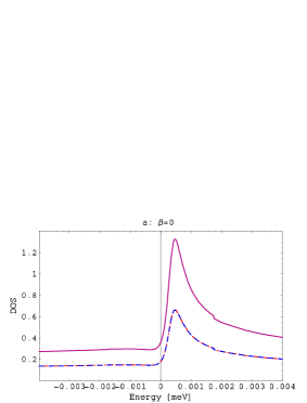
(a)  $\beta=0$

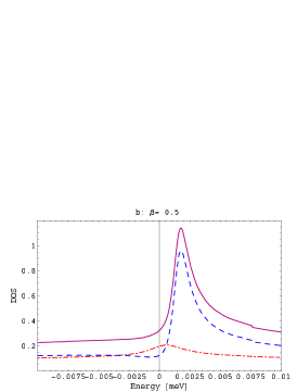
(b)  $\beta=0.5$

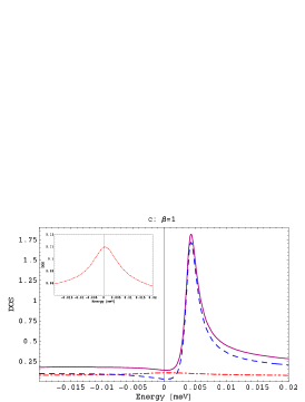
(c)  $\beta=1$

Figure 5: We plot the DOS with various $\beta$ values. Other parameters are $\Delta=0$, $\Gamma=0.2~{}\mathrm{meV}$, $D=10~{}\mathrm{meV}$, and $\varepsilon_{d}=-2~{}\mathrm{meV}$. In each graph, the red dot-dashed curve is plotted from the first term of Eq. 10, corresponding to $T_{K2}$, and the blue dashed curve from the second term, corresponding to $T_{K1}$. The purple solid curve is a combination of the two. (a) $\beta=0$, $T/T_{K1}(\beta=0)=0.6$, and $T_{K1}(\beta=0)=2.83\times 10^{-4}~{}\mathrm{meV}$. The red dot-dashed curve overlaps with the blue dashed curve as $T_{K1}=T_{K2}$ with the peaks located at $T_{K1}(\beta=0)$. (b)[(c)] $\beta=0.5[1]$, $T/T_{K1}(\beta=0.5[1])=0.6$. The blue dashed curve shifts right away from the Fermi level and its peak sits at $T_{K1}(\beta=0.5[1])=1.26\times 10^{-3}[3.88\times 10^{-3}]~{}\mathrm{meV}$, while the red dot-dashed curve shifts left towards the Fermi level with its peak located at $T_{K2}(\beta=0.5[1])=3.49\times 10^{-5}[1.51\times 10^{-6}]~{}\mathrm{meV}$. The inset in (c) shows the peak corresponding to $T_{K2}(\beta=1)$. Note that the blue dashed curve is more pronounced than the red dot-dashed curve because $T_{K1}>T_{K2}$ as $\beta>0$.

This enhancement of the Kondo peak and hence the Kondo temperature is caused by interference between two tunnelings, one with valley index conserved, and the other without.  This is evident from the fact that the $T_{K}$’s depend on the relative sign of $V_{0}$ and $V_{X}.$  Constructive interference increases the Kondo temperature whereas destructive interference decreases it. This $\beta$-dependent Kondo temperature is somewhat different from that in JSLim2006 , where the authors use slave-boson mean field theory. It would be interesting to investigate the difference between these two approaches. It should be mentioned that $T_{K}(\beta=0)$ acquired by the EOM approach underestimates the true Kondo temperature $T_{K}^{\ast}$ which is

$$k_{B}T_{K}^{\ast}=D\exp{(\pi\varepsilon_{m\sigma}/4\Gamma)}$$

This is certainly a deficiency of the EOM approach, and it has been discussed in the literature Lacroix1981 . The underestimation of the Kondo temperature from the EOM approach leads to its failure in determining, for example, the local spin susceptibility in the Kondo regime Kashcheyevs2006 . However, as we see in the following, the disappearance of Kondo peak structure suppressed by the temperature and the magnetic field is only scaled by the Kondo temperature $T_{K1(2)}(\beta)$ and hence the EOM approach faithfully captures the Kondo effect.

V V. Density of States

In Fig. 1 we showed the level structure of a single orbital on the QD.  The four energy states suffer both Zeeman splitting and valley splitting.  We now formally define these energies as $\varepsilon_{m\sigma}=\varepsilon_{d}+(\Delta/2+\mu_{v}B)(\delta_{m,e}-\delta_{m,o})+g\mu_{B}B(\delta_{\sigma,\uparrow}-\delta_{\sigma,\downarrow})$, where $\varepsilon_{d}$ is the bare energy of the dot and $B$ is the applied magnetic field. $\Delta$ is the zero-field valley splitting. Experiments in $2$-DEGs also show that the valley splitting increases linearly with the magnetic field srijit_nature . For a QD the valley splitting slope depends on the size of the dot. A small Si QD can have $\mu_{v}$ relatively comparable to $g\mu_{B}\sim 0.1~{}\mathrm{meV/T}$, with $g=2$.

In the following, we consider four different situations with different values of the three parameters $B,~{}\beta,~{}\Delta$ and in each discuss the peak structure in the DOS in full detail.  We have chosen the parameters $\Gamma=0.2$ meV, $D=10$ meV and $\varepsilon_{d}=-2$ meV.  This leads to rather low Kondo temperatures, but is favorable for illustration purposes.

V.1 A. $B=0$ and $\Delta=0$.

This is the case considered in the previous section.  $\Delta=0$ is probably not achievable in experiments, but this case is still important to understand, since it allows us to isolate the effect of valley index non-conservation. We showed in the previous section that there are two $\beta$-dependent Kondo peaks coming from the two terms of Eq. 10, the first term corresponding to $T_{K2}$, the second term corresponding to $T_{K1}$.   The DOS can be similarly partitioned, and we plot each piece separately together with their sum.  Fig. 5 shows the Kondo peak structure at $\beta=0,~{}0.5,~{}1$. We plot each graph at temperature $T=0.6~{}T_{K1}(\beta)$.  When $\beta=0$ (valley index conserved), $T_{K1}=T_{K2}$, the two Kondo peaks overlap with the peak position at $T_{K1}$, each contributing to half of the total weight. As $\beta$ increases and tunnelings between different valley states become allowed, $T_{K1}(\beta)$ increases with $\beta$, while $T_{K2}(\beta)$ decreases, according to Eq. 11 and 12. Since we set the temperature $T$ slightly smaller than $T_{K1}(\beta)$, but much larger than $T_{K2}(\beta=0.5,1)$, we expect to see one pronounced peak shift left and sit at energy $T_{K1}(\beta)$, and the other much suppressed peak shifts right towards $T_{K2}(\beta)$, as shown in Fig. 5. Therefore, when tunnelings between different valley states are allowed, it will enhance exponentially one Kondo peak with the Kondo temperature $T_{K1}$, and suppress exponentially the other Kondo peak with the Kondo temperature $T_{K2}$.   $T_{K1}$ overshadows $T_{K2}$ except in the neighborhood of $\beta=0.5$, where two peaks are relatively well separated and both sizable.  As stated above, it is probably difficult to achieve $\Delta=0$ experimentally.  However, even if $\Delta$ is small, we expect an enhancement of the upper Kondo temperature, making the features in the DOS associated with this $T_{K}$ easier to observe.  In this sense, Si is more favorable than GaAs for observation of the Kondo effect.

V.2 B. $B=0$, $\beta=0$.

Figure 6:  We plot the DOS with $\beta=0$, $B=0$ and $\Delta=0$(red solid curve), $\Delta=$$6~{}T_{K1}$(blue dot-dashed curve), and $\Delta=$$12~{}T_{K1}$(brown dotted curve) at a temperature $T=0.3~{}T_{K1}$ where $T_{K1}=2.83\times 10^{-4}~{}\mathrm{meV}$. The other parameters are the same as in Fig.  5. Note that at $\Delta=0$, the peak shifts slightly away from the Fermi level and locates itself at $T_{K1}$. As $\Delta$ increases, the peak splits into three peaks at the positions $-\Delta,~{}0,~{}\Delta$. The central peak comes from spin exchange at the same valley state (no energy penalty) and shifts back to the Fermi level, as expected from the conventional spin-$1/2$ Kondo effect. The other two side peaks result from inter-valley processes (energy cost $\Delta$). A schematic on the top left depicts two transitions that contribute to the central peak and left-side peak.

We now consider what happens when there is a finite valley splitting at zero field.  We find that there are three peaks in the DOS (and hence in the nonlinear conductance) instead of the usual two.  There is a central peak at zero energy and side peaks at $\pm\Delta.$  This is shown in Fig. 6.   The schematic diagram on the top left shows the conduction processes corresponding to the central peak and and the left-side peak. As clearly demonstrated in the schematic, there are basically two energetically distinguishable types of transitions, the inter-valley transition and the spin-flip transition at the same valley. Because valley degeneracy is already broken with a splitting $\Delta$, the inter-valley transitions cost an energy penalty $\Delta$, therefore shifting the peaks away from the Fermi level to $\pm\Delta$. They represent the transitions where an electron in the conduction bands enters into one valley state while an electron hops out of the QD from the other valley state (red dotted curve in the schematic). Furthermore, there is no energy cost in the spin-flip transition at the same valley, since spin degeneracy is still preserved, so the corresponding peak locates itself at the Fermi level (blue solid curve in the schematic). This is basically the same scenario as traditional spin-$1/2$ GaAs QDs. Fig. 7 shows that increase of temperature suppresses these three Kondo peaks equally, demonstrating that they are scaled by the same Kondo temperature.

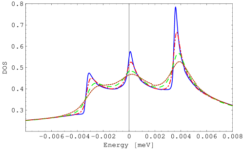
Figure 7: We plot the DOS with $\beta=0,~{}\Delta=12~{}T_{K1}$ at various temperatures: $T/T_{K1}=0.3$ (blue solid curve) , $T/T_{K1}=$$0.6$ (red dot-dashed curve), $T/T_{K1}=$$1.2$ (green dashed curve), and $T/T_{K1}=$ $1.8$ (brown dotted curve). The Kondo temperature $T_{K1}=2.84\times 10^{-4}~{}\mathrm{meV}$. The other parameters are the same as in Fig. 5. Here the three Kondo peaks are equally suppressed by increase of the temperature.

We further calculate the Kondo temperature with $\Delta\not=0$. Since $\beta=0$, we reduce the real part of the denominator of $\mathcal{G}_{m\sigma}$ to

$$w-\varepsilon_{m\sigma}-\sum_{l\not=m\sigma}\Sigma_{c,l}(z)=0$$ (13)

Consider $"m\sigma"="o\uparrow"$ energy state with the energy $\varepsilon_{o,\uparrow}=\varepsilon_{d}-\Delta/2$. As $T\rightarrow 0$, Eq. 13 can be rewritten as

$$w-\varepsilon_{d}+\Delta/2+\Gamma\mathrm{ln}\left|\frac{w}{D}\right|+2\Gamma\mathrm{ln}\left|\frac{w+\Delta}{D}\right|=0$$

Again we set $w=k_{B}T_{K}(\Delta)$. In the region $k_{B}T_{K}(\Delta=0)\ll|\Delta|\ll D$, because $T_{K}(\Delta\not=0)<T_{K}(\Delta=0)$, $k_{B}T_{K}(\Delta\not=0)\ll\Delta$. Therefore, we neglect linear $w$ and the last logarithmic term $2\Gamma\mathrm{ln}\left|\frac{w+\Delta}{D}\right|\sim 2\Gamma\mathrm{ln}\left|\frac{\Delta}{D}\right|$. We obtain

$$k_{B}T_{K}(\Delta) = D\exp((\varepsilon_{d}-\Delta/2)/\Gamma-2\mathrm{ln}\left|\Delta/D\right|)$$ (14)

$$= \frac{(k_{B}T_{K}(\Delta=0))^{3}}{\Delta^{2}}$$

Thus using EOM, we find $T_{K}(\Delta)\sim 1/\Delta^{2}$. Eto in his paper Eto2005 evaluates theoretically the Kondo temperature in the QDs with two orbitals and spin-$1/2$ as a function of $\Delta$, the energy difference between the two orbitals. He considers the case $\beta=0$ so the two Kondo temperatures coincide.  Using ”poor man’s” scaling method, he finds that within the region where $T_{K}(\Delta=0)\ll|\Delta|\ll D$, $T_{K}(\Delta)$ decreases as $\Delta$ increases, according to a power law

$$k_{B}T_{K}(\Delta)=k_{B}T_{K}(\Delta=0)\cdot(k_{B}T_{K}(\Delta=0)/|\Delta|)^{\gamma}$$

where $\gamma=1$. The discrepancy of Eq. 14 from Eto’s power law is again due to the deficiency of EOM approach to find the true Kondo temperature.

Interestingly, as $\Delta$ becomes larger, the side peaks shift further away from the Fermi level and we recover the conventional spin-$1/2$ Kondo effect, with one Kondo peak at the Fermi level. This is in agreement with Eto’s analysis Eto2005 .

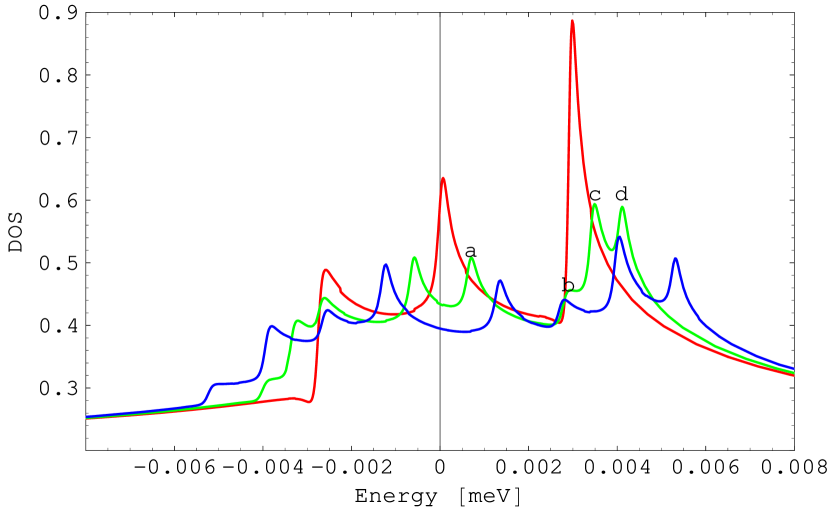
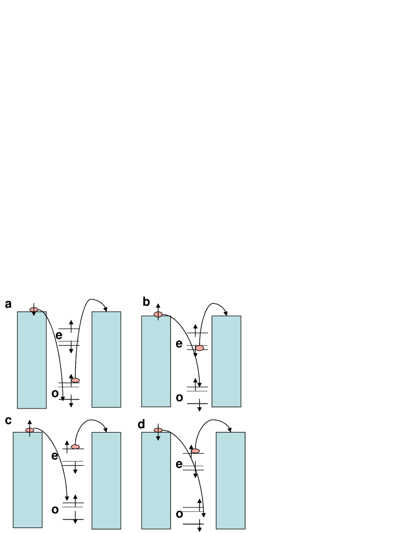
Figure 8: The DOS is plotted at $\beta=0$ with the magnetic field $B=0$ (red curve), $0.00284~{}\mathrm{T}$ (green curve) and $0.00568~{}\mathrm{T}$ (blue curve). The Kondo temperature $T_{K1}=2.84\times 10^{-4}~{}\mathrm{meV}$. We set $T/T_{K1}=0.2$. The other parameters are the same as in Fig. 5. We set $\mu_{v}=0.1~{}\mathrm{meV/T}$, slightly smaller than $g\mu_{B}=0.114~{}\mathrm{meV/T}$. The central peak splits into two peaks because the spin degeneracy is broken, while three energetically distinguishable inter-valley transitions due to the presence of magnetic field split the side peak into three peaks. The transitions that result in peaks $a,~{}b,~{}c,~{}d$(green curve) are shown in the schematic diagrams $a,~{}b,~{}c,~{}d$, respectively. Moreover, each peak evolves with a different slope with respect to the magnetic field due to cancellation or addition of spin and valley slopes. The slopes of peaks $a,~{}b,~{}c,~{}d$ are $0.228,~{}-0.028,~{}0.2,~{}0.428~{}\mathrm{meV/T}$, respectively.

V.3 C. $\beta=0$.

This is now the more general case of finite field and valley splitting, but still assuming that valley index is conserved.  Now the peak structure in the DOS becomes more complicated. As already seen in Fig. 6, at $B=0~{}$and $\Delta\not=0$, there are three peaks at $w=0,~{}\pm\Delta$. By applying a magnetic field, hence breaking spin degeneracy, as shown in Fig. 8, the central peak splits into two peaks with peak positions at $\pm 2g\mu_{B}B$ by Zeeman effect. In Fig. 8, the schematic diagram $a$ demonstrates a spin-flip transition that contributes to the peak at position $2g\mu_{B}B$. The side peak above the Fermi level splits into three peaks with peak positions at $\Delta+2(\mu_{v}-g\mu_{B})B,~{}\Delta+2\mu_{v}B,~{}\Delta+2(\mu_{v}+g\mu_{B})B$ which correspond to inter-valley transitions in the schematic diagrams $b,~{}c,~{}d$, respectively, whereas the side peak below the Fermi level also splits into three peaks with peak positions at $-\Delta-2(\mu_{v}+g\mu_{B})B,~{}-\Delta-2\mu_{v}B,~{}-\Delta-2(\mu_{v}-g\mu_{B})B$ by the same token. It is easy to see that twice the Zeeman energy $2g\mu_{B}B$ corresponds to the energy cost for spin-flip transitions, while valley splitting energy $\Delta+2\mu_{v}B$ corresponds to that for inter-valley transitions. The positions of these eight Kondo peaks have different dependencies on the magnetic field, with their slopes being expressed as various linear combinations of $\Delta,~{}\mu_{v}$, and $~{}g\mu_{B}$. It is worth noting that equally weighted peaks at positions $\pm\Delta\pm 2(\mu_{v}+g\mu_{B})B,~{}\pm\Delta\pm 2(\mu_{v}-g\mu_{B})B$ are twice as small as the other peaks because only half the number of conduction processes contribute to the peaks.

Figure 9: The Kondo peaks are shown with $B=0~{}T$ (red curve) and $B=0.0388~{}T$ (blue curve) when the valley index is not conserved. We consider $\beta=1$, $\Delta=8~{}T_{K1}~{}\mathrm{meV}$ and the Kondo temperature $T_{K1}=3.88\times 10^{-3}~{}\mathrm{meV}$. We set $T/T_{K1}=0.2$. The other parameters are the same as in Fig. 5. Note that there remains a peak at the Fermi level even when the magnetic field is not zero, in contrast to the peak structure when valley index is conserved (cf. Fig. 8). This peak comes from a transition where a conduction electron from an even valley state hops onto the dot at the odd valley state while the electron at the odd valley state hops out of the dot to a lead at an odd valley state, as shown in the top right schematic. This kind of transition costs no energy penalty.

V.4 D. $\beta=1$.

This is the case where tunneling between same valley states and different valley states are equally strong.  When the magnetic field is zero, there are three peaks near the Fermi level which we have explained in subsection B. However, as can be seen in Fig. 9, the central peak is more pronounced than the other two side peaks. This is due to extra contribution from tunnelings between different valley states. The effect of non-conservation of valley index can be seen more clearly when we apply a magnetic field. When $B\not=0$ and assuming the zero-field valley splitting $\Delta\not=0$, we saw eight peaks since spin and valley states are no longer degenerate. Surprisingly, as shown in Fig. 9, when the valley index is no longer conserved, we not only see the previous eight peaks as in Fig. 8 when the valley index is conserved, but also see an extra peak at the Fermi level that is independent of the magnetic field, meaning it can only be suppressed by increasing the temperature. This peak comes from a logarithmic divergence in the function $\Sigma_{d}(w)$ (cf. Eq. A.22) and is thus more pronounced as $\beta$ becomes larger. It also indicates that through cross-valley couplings $V_{X}$, $"m\sigma"$ and $"\bar{m}\sigma"$ form a bound state through exchanging electrons with the leads. The schematic in Fig. 9 demonstrates that this kind of transition through cross-valley couplings can occur without any energy cost. Consequently its peak sits at the Fermi level and has no dependence on the magnetic field.  This is in some sense the most characteristic signature that could be sought of the valley Kondo effect, since it results from a bound state of different valley states rather than different spin states.

VI VI. Conclusions and implications for experiments

Silicon quantum dots show a much richer phenomenology than GaAs dots due to the additional valley degree of freedom.  The initially fourfold degenerate level is split at zero applied magnetic field by interface effects and there is additional splitting at finite fields.  We have computed the density of states on the dot in the large-$U$ limit using an equation of motion method that has been shown to give reasonable results in related problems.  This function should closely mimic the non-linear conductance through the dot as a function of voltage.

The nonlinear conductance near zero bias of a Si QD with a single electron is sharply different from that of a GaAs QD in the Kondo regime:

1. At $B=0$ we expect three peaks near zero bias at $e\mathrm{V}=0,\pm\Delta,$ where $\Delta$ is the valley splitting.  The central peak is the spin Kondo peak while the other peaks correspond to inter-valley conduction processes.

2. For $B>0,$ the side peaks further split into three peaks, the two split-off peaks corresponding to spin-flip processes and the middle corresponding to spin conserving processes.

3. For $B>0,$ the central peak splits into two peaks if the valley index is conserved and three if it is not conserved, the latter corresponding to a valley-Kondo ground state.

4. The temperature dependence can be complex, since there are two Kondo temperatures in the problem.

5. The conservation or non-conservation of valley index depends quite sensitively on the precise details of the junctions and is therefore likely to be sample-dependent and difficult to control.

We hope that some or all of these phenomena will be observed in future experiments.

VII Acknowledgements

We gratefully acknowledge conversations with M. Friesen.  This work was supported by NSA and ARDA under ARO contract number W911NF-04-1-0389 and by the National Science Foundation through the ITR (DMR-0325634) and EMT (CCF-0523675) programs.

APPENDIX: EOM FOR INFINITE $U$

The basic equations of motion for the Green’s functions are

$$(w-\varepsilon_{m\sigma})\ll f_{m\sigma},f_{m\sigma}^{+}\gg = 1+\sum_{ik}V_{0,ik}\ll c_{ikm\sigma},f_{m\sigma}^{+}\gg+\sum_{ik}V_{X,ik}\ll c_{ik\bar{m}\sigma},f_{m\sigma}^{+}\gg$$

$$+U\sum_{l\not=m\sigma}\ll f_{l}^{+}f_{l}f_{m\sigma},f_{m\sigma}^{+}\gg.$$

$$(w-\varepsilon_{k})\ll c_{ikm\sigma},f_{m\sigma}^{+}\gg = V_{0,ik}\ll f_{m\sigma},f_{m\sigma}^{+}\gg+V_{X,ik}\ll f_{\bar{m}\sigma},f_{m\sigma}^{+}\gg.$$

$$(w-\varepsilon_{\bar{m}\sigma})\ll f_{\bar{m}\sigma},f_{m\sigma}^{+}\gg = \sum_{ik}V_{0,ik}\ll c_{ik\bar{m}\sigma},f_{m\sigma}^{+}\gg+\sum_{ik}V_{X,ik}\ll c_{ikm\sigma},f_{m\sigma}^{+}\gg$$

$$+U\sum_{p\not=\bar{m}\sigma}\ll f_{p}^{+}f_{p}f_{\bar{m}\sigma},f_{m\sigma}^{+}\gg.$$

$$(w-\varepsilon_{k})\ll c_{ik\bar{m}\sigma},f_{m\sigma}^{+}\gg = V_{0,ik}\ll f_{\bar{m}\sigma},f_{m\sigma}^{+}\gg+V_{X,ik}\ll f_{m\sigma},f_{m\sigma}^{+}\gg.$$

Note that $l,p$ are shorthand for valley plus spin indices, unlike $m$ that means only the valley index. Furthermore if $l=m\sigma$, $\bar{l}=\bar{m}\sigma$. The bar means exchanging only the valley index. From now on we simplify the calculation by changing $V_{0(X),ik}\rightarrow V_{0(X)}$. From the above four coupled equations of motion we can obtain

$$(w-\varepsilon_{m\sigma}-\sum_{ik}\frac{V_{0}^{2}+V_{X}^{2}}{w-\varepsilon_{k}})\ll f_{m\sigma},f_{m\sigma}^{+}\gg = 1+\sum_{ik}\frac{2V_{0}V_{X}}{w-\varepsilon_{k}}\ll f_{\bar{m}\sigma},f_{m\sigma}^{+}\gg$$ (A.1)

$$+U\sum_{l\not=m\sigma}\ll f_{l}^{+}f_{l}f_{m\sigma},f_{m\sigma}^{+}\gg$$

$$(w-\varepsilon_{\bar{m}\sigma}-\sum_{ik}\frac{V_{0}^{2}+V_{X}^{2}}{w-\varepsilon_{k}})\ll f_{\bar{m}\sigma},f_{m\sigma}^{+}\gg = \sum_{ik}\frac{2V_{0}V_{X}}{w-\varepsilon_{k}}\ll f_{m\sigma},f_{m\sigma}^{+}\gg$$ (A.2)

$$+U\sum_{p\not=\bar{m}\sigma}\ll f_{p}^{+}f_{p}f_{\bar{m}\sigma},f_{m\sigma}^{+}\gg$$

The higher-order terms give rise to

$$(w-\varepsilon_{m\sigma}-U)\ll n_{l}f_{m\sigma},f_{m\sigma}^{+}\gg = <n_{l}>+\sum_{ik}V_{0}\{\ll n_{l}c_{ikm\sigma},f_{m\sigma}^{+}\gg+\ll f_{l}^{+}c_{ikl}f_{m\sigma},f_{m\sigma}^{+}\gg$$ (A.3)

$$-\ll c_{ikl}^{+}f_{l}f_{m\sigma},f_{m\sigma}^{+}\gg\}+\sum_{ik}V_{X}\{\ll n_{l}c_{ik\bar{m}\sigma},f_{m\sigma}^{+}\gg$$

$$+\ll f_{l}^{+}c_{ik\bar{l}}f_{m\sigma},f_{m\sigma}^{+}\gg-\ll c_{ik\bar{l}}^{+}f_{l}f_{m\sigma},f_{m\sigma}^{+}\gg\}$$

$$+U\sum_{j\not=l\not=m\sigma}\ll n_{l}n_{j}f_{m\sigma},f_{m\sigma}^{+}\gg$$

$$(w-\varepsilon_{\bar{m}\sigma}-U)\ll n_{p}f_{\bar{m}\sigma},f_{m\sigma}^{+}\gg = -\delta_{p,m\sigma}<f_{m\sigma}^{+}f_{\bar{m}\sigma}>+\sum_{ik}V_{0}\{\ll n_{p}c_{ik\bar{m}\sigma},f_{m\sigma}^{+}\gg$$ (A.4)

$$+\ll f_{p}^{+}c_{ikp}f_{\bar{m}\sigma},f_{m\sigma}^{+}\gg-\ll c_{ikp}^{+}f_{p}f_{\bar{m}\sigma},f_{m\sigma}^{+}\gg\}$$

$$+\sum_{ik}V_{X}\{\ll n_{p}c_{ikm\sigma},f_{m\sigma}^{+}\gg+\ll f_{p}^{+}c_{ik\bar{p}}f_{\bar{m}\sigma},f_{m\sigma}^{+}\gg$$

$$-\ll c_{ik\bar{p}}^{+}f_{p}f_{\bar{m}\sigma},f_{m\sigma}^{+}\gg\}+U\sum_{j\not=p\not=\bar{m}\sigma}\ll n_{j}n_{p}f_{\bar{m}\sigma},f_{m\sigma}^{+}\gg$$

Next, we proceed to obtain equations of motion for the higher-order functions appearing on the right-hand side of Eq. A.3 and Eq. A.4

$$(w-\varepsilon_{k})\ll n_{l}c_{ikm\sigma},f_{m\sigma}^{+}\gg = -\delta_{l,m\sigma}<f_{m\sigma}^{+}c_{ikm\sigma}>+V_{0}\{\ll n_{l}f_{m\sigma},f_{m\sigma}^{+}\gg$$ (A.5)

$$-\sum_{i^{\prime}k^{\prime}}\ll c_{i^{\prime}k^{\prime}l}^{+}f_{l}c_{ikm\sigma},f_{m\sigma}^{+}\gg+\sum_{i^{\prime}k^{\prime}}\ll f_{l}^{+}c_{i^{\prime}k^{\prime}l}c_{ikm\sigma},f_{m\sigma}^{+}\gg\}$$

$$+V_{X}\{\ll n_{l}f_{\bar{m}\sigma},f_{m\sigma}^{+}\gg-\sum_{i^{\prime}k^{\prime}}\ll c_{i^{\prime}k^{\prime}\bar{l}}^{+}f_{l}c_{ikm\sigma},f_{m\sigma}^{+}\gg$$

$$+\sum_{i^{\prime}k^{\prime}}\ll f_{l}^{+}c_{i^{\prime}k^{\prime}\bar{l}}c_{ikm\sigma},f_{m\sigma}^{+}\gg\}$$

$$(w-\varepsilon_{k})\ll n_{l}c_{ik\bar{m}\sigma},f_{m\sigma}^{+}\gg = -\delta_{l,m\sigma}<f_{m\sigma}^{+}c_{ik\bar{m}\sigma}>+V_{0}\{\ll n_{l}f_{\bar{m}\sigma},f_{m\sigma}^{+}\gg$$ (A.6)

$$-\sum_{i^{\prime}k^{\prime}}\ll c_{i^{\prime}k^{\prime}l}^{+}f_{l}c_{ik\bar{m}\sigma},f_{m\sigma}^{+}\gg+\sum_{i^{\prime}k^{\prime}}\ll f_{l}^{+}c_{i^{\prime}k^{\prime}l}c_{ik\bar{m}\sigma},f_{m\sigma}^{+}\gg\}$$

$$+V_{X}\{\ll n_{l}f_{m\sigma},f_{m\sigma}^{+}\gg-\sum_{i^{\prime}k^{\prime}}\ll c_{i^{\prime}k^{\prime}\bar{l}}^{+}f_{l}c_{ik\bar{m}\sigma},f_{m\sigma}^{+}\gg$$

$$+\sum_{i^{\prime}k^{\prime}}\ll f_{l}^{+}c_{i^{\prime}k^{\prime}\bar{l}}c_{ik\bar{m}\sigma},f_{m\sigma}^{+}\gg\}$$

$$(z-\varepsilon_{k})\ll f_{l}^{+}c_{ikl}f_{m\sigma},f_{m\sigma}^{+}\gg = <f_{l}^{+}c_{ikl}>+V_{0}\{\ll f_{l}^{+}f_{l}f_{m\sigma},f_{m\sigma}^{+}\gg-\sum_{i^{\prime}k^{\prime}}\ll c_{i^{\prime}k^{\prime}l}^{+}c_{ikl}f_{m\sigma},f_{m\sigma}^{+}\gg$$ (A.7)

$$-\sum_{i^{\prime}k^{\prime}}\ll c_{ikl}f_{l}^{+}c_{i^{\prime}k^{\prime}m\sigma},f_{m\sigma}^{+}\gg\}+V_{X}\{\ll f_{l}^{+}f_{\bar{l}}f_{m\sigma},f_{m\sigma}^{+}\gg$$

$$-\sum_{i^{\prime}k^{\prime}}\ll c_{i^{\prime}k^{\prime}\bar{l}}^{+}c_{ikl}f_{m\sigma},f_{m\sigma}^{+}\gg-\sum_{i^{\prime}k^{\prime}}\ll c_{ikl}f_{l}^{+}c_{i^{\prime}k^{\prime}\bar{m}\sigma},f_{m\sigma}^{+}\gg\}$$

$$(z-\varepsilon_{k})\ll f_{l}^{+}c_{ik\bar{l}}f_{m\sigma},f_{m\sigma}^{+}\gg = <f_{l}^{+}c_{ik\bar{l}}>+V_{0}\{\ll f_{l}^{+}f_{\bar{l}}f_{m\sigma},f_{m\sigma}^{+}\gg-\sum_{i^{\prime}k^{\prime}}\ll c_{i^{\prime}k^{\prime}l}^{+}c_{ik\bar{l}}f_{m\sigma},f_{m\sigma}^{+}\gg$$ (A.8)

$$-\sum_{i^{\prime}k^{\prime}}\ll c_{ik\bar{l}}f_{l}^{+}c_{i^{\prime}k^{\prime}m\sigma},f_{m\sigma}^{+}\gg\}+V_{X}\{\ll f_{l}^{+}f_{l}f_{m\sigma},f_{m\sigma}^{+}\gg$$

$$-\sum_{i^{\prime}k^{\prime}}\ll c_{i^{\prime}k^{\prime}\bar{l}}^{+}c_{ik\bar{l}}f_{m\sigma},f_{m\sigma}^{+}\gg-\sum_{i^{\prime}k^{\prime}}\ll c_{ik\bar{l}}f_{l}^{+}c_{i^{\prime}k^{\prime}\bar{m}\sigma},f_{m\sigma}^{+}\gg\}$$

$$\ll c_{ikl}^{+}f_{l}f_{m\sigma},f_{m\sigma}^{+}\gg \sim 1/(w+\varepsilon_{k}-\varepsilon_{l}-\varepsilon_{m\sigma}-U)$$ (A.9)

$$\ll c_{ik\bar{l}}^{+}f_{l}f_{m\sigma},f_{m\sigma}^{+}\gg \sim 1/(w+\varepsilon_{k}-\varepsilon_{l}-\varepsilon_{m\sigma}-U)$$ (A.10)

$$U\ll n_{l}n_{j}f_{m\sigma},f_{m\sigma}^{+}\gg = U(<n_{l}n_{j}>+\cdots)/(w-\varepsilon_{m\sigma}-2U)$$ (A.11)

$$(\bar{z}-\varepsilon_{k})\ll f_{l}^{+}c_{ikl}f_{\bar{m}\sigma},f_{m\sigma}^{+}\gg = V_{0}\{\ll f_{l}^{+}f_{l}f_{\bar{m}\sigma},f_{m\sigma}^{+}\gg-\sum_{i^{\prime}k^{\prime}}\ll c_{i^{\prime}k^{\prime}l}^{+}c_{ikl}f_{\bar{m}\sigma},f_{m\sigma}^{+}\gg$$ (A.12)

$$-\sum_{i^{\prime}k^{\prime}}\ll c_{ikl}f_{l}^{+}c_{i^{\prime}k^{\prime}\bar{m}\sigma},f_{m\sigma}^{+}\gg\}+V_{X}\{\ll f_{l}^{+}f_{\bar{l}}f_{\bar{m}\sigma},f_{m\sigma}^{+}\gg$$

$$-\sum_{i^{\prime}k^{\prime}}\ll c_{i^{\prime}k^{\prime}\bar{l}}^{+}c_{ikl}f_{\bar{m}\sigma},f_{m\sigma}^{+}\gg-\sum_{i^{\prime}k^{\prime}}\ll c_{ikl}f_{l}^{+}c_{i^{\prime}k^{\prime}m\sigma},f_{m\sigma}^{+}\gg\}$$

$$(\bar{z}-\varepsilon_{k})\ll f_{l}^{+}c_{ik\bar{l}}f_{\bar{m}\sigma},f_{m\sigma}^{+}\gg = V_{0}\{\ll f_{l}^{+}f_{\bar{l}}f_{\bar{m}\sigma},f_{m\sigma}^{+}\gg-\sum_{i^{\prime}k^{\prime}}\ll c_{i^{\prime}k^{\prime}l}^{+}c_{ik\bar{l}}f_{\bar{m}\sigma},f_{m\sigma}^{+}\gg$$ (A.13)

$$-\sum_{i^{\prime}k^{\prime}}\ll c_{ik\bar{l}}f_{l}^{+}c_{i^{\prime}k^{\prime}\bar{m}\sigma},f_{m\sigma}^{+}\gg\}+V_{X}\{\ll f_{l}^{+}f_{l}f_{\bar{m}\sigma},f_{m\sigma}^{+}\gg$$

$$-\sum_{i^{\prime}k^{\prime}}\ll c_{i^{\prime}k^{\prime}\bar{l}}^{+}c_{ik\bar{l}}f_{\bar{m}\sigma},f_{m\sigma}^{+}\gg-\sum_{i^{\prime}k^{\prime}}\ll c_{ik\bar{l}}f_{l}^{+}c_{i^{\prime}k^{\prime}m\sigma},f_{m\sigma}^{+}\gg\}$$

$$\ll c_{ikl}^{+}f_{l}f_{\bar{m}\sigma},f_{m\sigma}^{+}\gg \sim 1/(w+\varepsilon_{k}-\varepsilon_{l}-\varepsilon_{\bar{m}\sigma}-U)$$ (A.14)

$$\ll c_{ik\bar{l}}^{+}f_{l}f_{\bar{m}\sigma},f_{m\sigma}^{+}\gg \sim 1/(w+\varepsilon_{k}-\varepsilon_{l}-\varepsilon_{\bar{m}\sigma}-U)$$ (A.15)

$$U\ll n_{l}n_{j}f_{\bar{m}\sigma},f_{m\sigma}^{+}\gg = U(\delta_{l,m\sigma}<n_{j}f_{m\sigma}^{+}f_{\bar{m}\sigma}>+\cdots)/(w-\varepsilon_{\bar{m}\sigma}-2U).$$ (A.16)

Note $z=w-\varepsilon_{m\sigma}+\varepsilon_{l\not=m\sigma}$ and $\bar{z}=w-\varepsilon_{\bar{m}\sigma}+\varepsilon_{l\not=\bar{m}\sigma}$.  If we take $U\rightarrow\infty$, Eq. A.9-A.11 and Eq. A.14-A.16 vanish, as do correlators And the rest involving two annihilation operators on the dot like $\ll f_{l}^{+}f_{\bar{l}}f_{m\sigma},f_{m\sigma}^{+}\gg$ also vanish as $U\rightarrow\infty$. After we truncate the higher-order Green’s functions, we will encounter related integrals that by simple manipulation we transform into integrals over Green’s functions $\ll f_{m\sigma},f_{m\sigma}^{+}\gg(\mathcal{G}_{m\sigma})$ and $\ll f_{\bar{m}\sigma},f_{m\sigma}^{+}\gg(\mathcal{M}_{\bar{m}\sigma})$. Thus the set of EOM terminates after truncation and the Green’s function $\mathcal{G}_{m\sigma}$ can be solved for. The equations are

$$\sum_{ik,i^{\prime}k^{\prime}}\frac{<c_{i^{\prime}k^{\prime}\bar{m}\sigma}^{+}c_{ikm\sigma}>}{z-\varepsilon_{k}} = -\frac{4}{4\pi D^{2}}\int_{-D}^{D}d\varepsilon\int_{-D}^{D}d\varepsilon^{\prime}\int dw^{\prime}f_{FD}(w^{\prime})\frac{\mathrm{Im}\ll c_{ikm\sigma},c_{i^{\prime}k^{\prime}\bar{m}\sigma}^{+}\gg_{w^{\prime}+i\delta}}{z-\varepsilon}$$

$$= \frac{-i\pi}{D^{2}}(V_{0}^{2}\tilde{B}_{m\sigma,\bar{m}\sigma}(z)+V_{X}^{2}\tilde{B}_{\bar{m}\sigma,m\sigma}(z)+V_{0}V_{X}(\tilde{B}_{m\sigma,m\sigma}(z)+\tilde{B}_{\bar{m}\sigma,\bar{m}\sigma}(z))).$$

$$\sum_{ik,i^{\prime}k^{\prime}}\frac{<c_{i^{\prime}k^{\prime}m\sigma}^{+}c_{ikm\sigma}>}{z-\varepsilon_{k}} = -\frac{2}{2D}\int_{-D}^{D}dw^{\prime}\frac{f_{FD}(w^{\prime})}{w^{\prime}-z-i\delta}+\frac{-i\pi}{D^{2}}(V_{0}^{2}\tilde{B}_{m\sigma,m\sigma}(z)+V_{X}^{2}\tilde{B}_{\bar{m}\sigma,\bar{m}\sigma}(z)$$

$$+V_{0}V_{X}(\tilde{B}_{m\sigma,\bar{m}\sigma}(z)+\tilde{B}_{\bar{m}\sigma,m\sigma}(z))).$$

$$\sum_{ik}\frac{<f_{m\sigma}^{+}c_{ikm\sigma}>}{z-\varepsilon_{k}} = \frac{-2}{2D}(V_{0}\tilde{B}_{m\sigma,m\sigma}(z))+V_{X}\tilde{B}_{\bar{m}\sigma,m\sigma}(z)).$$

$$\sum_{ik}\frac{<f_{m\sigma}^{+}c_{ik\bar{m}\sigma}>}{z-\varepsilon_{k}} = \frac{-2}{2D}(V_{0}\tilde{B}_{\bar{m}\sigma,m\sigma}(z))+V_{X}\tilde{B}_{m\sigma,m\sigma}(z)).$$

$$\sum_{ik}\frac{<c_{ikm\sigma}^{+}f_{m\sigma}>}{z-\varepsilon_{k}} = \frac{-2}{2D}(V_{0}\tilde{B}_{m\sigma,m\sigma}(z))+V_{X}\tilde{B}_{m\sigma,\bar{m}\sigma}(z)).$$

$$\sum_{ik}\frac{<c_{ik\bar{m}\sigma}^{+}f_{m\sigma}>}{z-\varepsilon_{k}} = \frac{-2}{2D}(V_{0}\tilde{B}_{m\sigma,\bar{m}\sigma}(z))+V_{X}\tilde{B}_{m\sigma,m\sigma}(z)).$$

with

$$\tilde{B}_{\alpha,\beta}(w)=\int_{-D}^{D}dw^{\prime}f_{FD}(w^{\prime})\frac{\ll f_{\alpha},f_{\beta}^{+}\gg^{\ast}}{w^{\prime}-w-i\delta}$$

Note that we have considered both the correlations in the conduction bands, and on the dot. However, conduction electrons do not mix different valley states except through cross-valley couplings ($V_{X}$) with the dot. Thus terms like $\sum_{i^{\prime}k^{\prime},ik}\frac{<c_{i^{\prime}k^{\prime}\bar{l}}^{+}c_{ikl}>}{w-\varepsilon_{k}}$ are of order $V_{0(X)}^{2}$, while terms such as $\sum_{ik}\frac{<f_{l}^{+}c_{ik\bar{l}}>}{w-\varepsilon_{k}}$ are of order $V_{0(X)}$. Eq. A.3 and A.4 can be thus expressed as

$$(w-\varepsilon_{m\sigma}-U-\Sigma_{a}(w)-\Sigma_{a}(z))\ll n_{l}f_{m\sigma},f_{m\sigma}^{+}\gg=\Sigma_{b}(w)\ll n_{l}f_{\bar{m}\sigma},f_{m\sigma}^{+}\gg_{l\not=\bar{m}\sigma}$$

$$+\{\delta_{l,\bar{m}\sigma}(\widetilde{I}_{m\sigma}(w)-\Sigma_{a}(w)\widetilde{F}_{m\sigma}(w)+\Sigma_{d}(w))+\Sigma_{b}(w)\tilde{A}_{l}(z)\}\mathcal{M}_{\bar{m}\sigma}$$

$$+\{-\delta_{l,\bar{m}\sigma}\Sigma_{b}(w)\widetilde{F}_{m\sigma}(w)+\Sigma_{a}(w)\tilde{A}_{l}(z)-\Sigma_{c,l}(z)-\widetilde{J}_{l}(z)\}\mathcal{G}_{m\sigma}+<n_{l}>+\tilde{A}_{l}(z)$$ (A.17)

$$(w-\varepsilon_{\bar{m}\sigma}-U-\Sigma_{a}(w)-\Sigma_{a}(\bar{z}))\ll n_{p}f_{\bar{m}\sigma},f_{m\sigma}^{+}\gg=\Sigma_{b}(w)\ll n_{p}f_{m\sigma},f_{m\sigma}^{+}\gg_{p\not=m\sigma}$$

$$-\delta_{p,m\sigma}<f_{m\sigma}^{+}f_{\bar{m}\sigma}>-\delta_{p,m\sigma}\widetilde{\bar{F}}_{m\sigma}(w)+\{\delta_{p,m\sigma}(\widetilde{\bar{I}}_{m\sigma}(w)-\Sigma_{a}(w)\widetilde{\bar{F}}_{m\sigma}(w)+\Sigma_{d}(w))$$

$$+\Sigma_{b}(w)\tilde{A}_{p}(\bar{z})\}\mathcal{G}_{m\sigma}+\{-\delta_{p,m\sigma}\Sigma_{b}(w)\widetilde{\bar{F}}_{m\sigma}(w)+\Sigma_{a}(w)\tilde{A}_{p}(\bar{z})-\Sigma_{c,p}(\bar{z})-\widetilde{J}_{p}(\bar{z})\}\mathcal{M}_{\bar{m}\sigma}$$ (A.18)

where the various functions are defined by

$$\Sigma_{a}(w) = \sum_{ik}\frac{V_{0}^{2}+V_{X}^{2}}{w-\varepsilon_{k}}$$ (A.19)

$$\Sigma_{b}(w) = \sum_{ik}\frac{2V_{0}V_{X}}{w-\varepsilon_{k}}$$ (A.20)

$$\Sigma_{c,l}(z) = \sum_{i^{\prime}k^{\prime}ik}\frac{(V_{0}^{2}+V_{X}^{2})<c_{i^{\prime}k^{\prime}l}^{+}c_{ikl}>}{z-\varepsilon_{k}}$$ (A.21)

$$= -\frac{2}{2D}\int_{-D}^{D}dw^{\prime}f_{FD}(w^{\prime})\frac{V_{0}^{2}+V_{X}^{2}}{w^{\prime}-z-i\delta}+\frac{-\pi(V_{0}^{2}+V_{X}^{2})i}{D^{2}}(V_{0}^{2}\tilde{B}_{l,l}(z)+V_{X}^{2}\tilde{B}_{\bar{l},\bar{l}}(z)$$

$$+V_{0}V_{X}(\tilde{B}_{l,\bar{l}}(z)+\tilde{B}_{\bar{l},l}(z))).$$

$$\Sigma_{d}(w) = \sum_{ik,i^{\prime}k^{\prime}}\frac{2V_{0}V_{X}<c_{i^{\prime}k^{\prime}m\sigma}^{+}c_{ikm\sigma}>}{w-\varepsilon_{k}}$$ (A.22)

$$= -\frac{2}{2D}\int_{-D}^{D}dw^{\prime}f_{FD}(w^{\prime})\frac{2V_{0}V_{X}}{w^{\prime}-w-i\delta}+\frac{-2\pi V_{0}V_{X}i}{D^{2}}(V_{0}^{2}\tilde{B}_{m\sigma,m\sigma}(w)+V_{X}^{2}\tilde{B}_{\bar{m}\sigma,\bar{m}\sigma}(w)$$

$$+V_{0}V_{X}(\tilde{B}_{m\sigma,\bar{m}\sigma}(w)+\tilde{B}_{\bar{m}\sigma,m\sigma}(w))).$$

$$\widetilde{I}_{m\sigma}(w) = \sum_{i^{\prime}k^{\prime}ik}\frac{V_{0}^{2}<c_{i^{\prime}k^{\prime}\bar{m}\sigma}^{+}c_{ikm\sigma}>+V_{X}^{2}<c_{i^{\prime}k^{\prime}m\sigma}^{+}c_{ik\bar{m}\sigma}>}{w-\varepsilon_{k}}$$ (A.23)

$$= \frac{-i\pi}{D^{2}}((V_{0}^{4}+V_{X}^{4})\tilde{B}_{m\sigma,\bar{m}\sigma}(w)+2V_{0}^{2}V_{X}^{2}\tilde{B}_{\bar{m}\sigma,m\sigma}(w)$$

$$+(V_{0}^{2}+V_{X}^{2})V_{0}V_{X}(\tilde{B}_{m\sigma,m\sigma}(w)+\tilde{B}_{\bar{m}\sigma,\bar{m}\sigma}(w))).$$

$$\widetilde{F}_{m\sigma}(w) = \sum_{ik}\frac{V_{0}<f_{\bar{m}\sigma}^{+}c_{ikm\sigma}>+V_{X}<f_{\bar{m}\sigma}^{+}c_{ik\bar{m}\sigma}>}{w-\varepsilon_{k}}$$ (A.24)

$$= \frac{-2}{2D}((V_{0}^{2}+V_{X}^{2})\tilde{B}_{m\sigma,\bar{m}\sigma}(w)+2V_{0}V_{X}\tilde{B}_{\bar{m}\sigma,\bar{m}\sigma}(w)).$$

$$\widetilde{J}_{l}(z) = \sum_{i^{\prime}k^{\prime}ik}\frac{V_{0}V_{X}(<c_{i^{\prime}k^{\prime}\bar{l}}^{+}c_{ikl}>+<c_{i^{\prime}k^{\prime}l}^{+}c_{ik\bar{l}}>)}{z-\varepsilon_{k}}$$ (A.25)

$$= \frac{-i\pi}{D^{2}}V_{0}V_{X}((V_{0}^{2}+V_{X}^{2})(\tilde{B}_{\bar{l},l}(z)+\tilde{B}_{l,\bar{l}}(z))+2V_{0}V_{X}(\tilde{B}_{l,l}(z)+\tilde{B}_{\bar{l},\bar{l}}(z))).$$

$$\tilde{A}_{l}(z) = \sum_{ik}\frac{V_{X}<f_{l}^{+}c_{ik\bar{l}}>+V_{0}<f_{l}^{+}c_{ikl}>}{z-\varepsilon_{k}}$$ (A.26)

$$= \frac{-2}{2D}((V_{0}^{2}+V_{X}^{2})\tilde{B}_{l,l}(z)+2V_{0}V_{X}\tilde{B}_{\bar{l},l}(z)).$$

$$\widetilde{\bar{I}}_{m\sigma}(w) = \sum_{i^{\prime}k^{\prime}ik}\frac{V_{0}^{2}<c_{i^{\prime}k^{\prime}m\sigma}^{+}c_{ik\bar{m}\sigma}>+V_{X}^{2}<c_{i^{\prime}k^{\prime}\bar{m}\sigma}^{+}c_{ikm\sigma}>}{w-\varepsilon_{k}}$$ (A.27)

$$= \frac{-i\pi}{D^{2}}((V_{0}^{4}+V_{X}^{4})\tilde{B}_{\bar{m}\sigma,m\sigma}(w)+2V_{0}^{2}V_{X}^{2}\tilde{B}_{m\sigma,\bar{m}\sigma}(w)$$

$$+(V_{0}^{2}+V_{X}^{2})V_{0}V_{X}(\tilde{B}_{m\sigma,m\sigma}(w)+\tilde{B}_{\bar{m}\sigma,\bar{m}\sigma}(w))).$$

$$\widetilde{\bar{F}}_{m\sigma}(w) = \sum_{ik}\frac{V_{0}<f_{m\sigma}^{+}c_{ik\bar{m}\sigma}>+V_{X}<f_{m\sigma}^{+}c_{ikm\sigma}>}{w-\varepsilon_{k}}$$ (A.28)

$$= \frac{-2}{2D}((V_{0}^{2}+V_{X}^{2})\tilde{B}_{\bar{m}\sigma,m\sigma}(w)+2V_{0}V_{X}\tilde{B}_{m\sigma,m\sigma}(w)).$$

Combining Eq. A.1, A.2, A.17, A.18, and taking the limit $U\rightarrow\infty$, we obtain Eq. 7 in the main text.

References

- (1) W. Jantsch et al, Physica E 13, 504 (2002); Z. Wilamowski et al Physica E 16, 111 (2003).
- (2) A. M. Tyryshkin, S. A. Lyon, W. Jantsch, F. Schaeffler, Phys. Rev. Lett. 94, 126802 (2005).
- (3) A. M. Tyryshkin, S. A. Lyon, W. Jantsch, F. Schaeffler, Phys. Rev. B 68, 193207 (2003).
- (4) R. de Sousa and S. Das Sarma, Phys. Rev. B 68, 115322 (2003)
- (5) M. A. Eriksson et al. Quantum Information Processing 3, 133 (2004).
- (6) G. M. Jones et al. Appl. Phys. Lett. 89, 073106 (2006).
- (7) L. J. Klein et al. Appl. Phys. Lett. 84, 4047 (2004).
- (8) S. Goswami et al., cond-mat/0611221. To appear in Nature Physics.
- (9) T. B. Boykin et al. Phys. Rev. B 70, 165325 (2004).
- (10) T. B. Boykin et al. Appl. Phys. Lett. 84, 115 (2004).
- (11) F. J. Ohkawa and Y. Uemura, Journ. Phys. Soc. Japan, 43, 925 (1977).
- (12) M. Friesen, S. Chutia, C. Tahan, and S.N. Coppersmith, cond-mat/0608229.
- (13) Mark Friesen, M. A. Eriksson, and S. N. Coppersmith, cond-mat/0602194.
- (14) D. Goldhaber-Gordon et al. Nature 391, 156 (1998).
- (15) P. Jarillo-Herrero et al. Nature(London) 434, 484 (2005).
- (16) M.-S. Choi et al. Phys. Rev. Lett. 95, 067204 (2005).
- (17) S. Sasaki et al. Phys. Rev. Lett. 93, 017205 (2004).
- (18) L. P. Rokhinson, L. J. Guo, S. Y. Chou, and D. C. Tsui, Phys. Rev B 60, R16319 (1999)
- (19) J. S. Lim et al. cond-mat/0608110.
- (20) T. Inoshita et al., Phys. Rev. B 48, 14725 (1993); T. Pohjola et al., Europhys. Lett. 40, 189 (1997); A. Levy Yeyati et al., Phys. Rev. Lett. 83, 600 (1999); R. Sakano and N. Kawakami, Phys. Rev. B 73, 155332 (2006).
- (21) A. L. Chudnovskiy, Europhys. Lett. 71, 672 (2005).
- (22) R. Landauer, Philos. Mag. 21, 863 (1970).
- (23) G. Czycholl, Phys. Rev. B 31, 2867 (1985).
- (24) C. Lacroix, J. Phys. F. 11, 2389 (1981).
- (25) H.-G. Luo, S.-J. Wang, and C.-L. Jia, Phys. Rev. B 66, 235311 (2002).
- (26) V. Kashcheyevs, A. Aharony, and O. Entin-Wohlman, Phys. Rev. B 73, 125338 (2006).
- (27) In the case where , mathematically there is no constraint to the magnitude of and when iterating the computation to determine their values. However, note that the value should be approximately of order . Since the stability doesn’t reach at , we first stablize by setting in a sense that we treat perturbatively. Afterwards we iterate to determine and stop when it reaches a value and take both values to plot the DOS.
- (28) A.P. Hewson, The Kondo Problem to Heavy Fermions, (Cambridge Univ. Press, Cambridge, 1993), Sec. 7.2.
- (29) M. Eto, J. Phys. Soc. Jpn. 74, 95 (2005).