A thermodynamical fiber bundle model for the fracture of disordered materials

Abstract

We investigate a disordered version of a thermodynamic fiber bundle model proposed by Selinger, Wang, Gelbart, and Ben-Shaul a few years ago. For simple forms of disorder, the model is analytically tractable and displays some new features. At either constant stress or constant strain, there is a non monotonic increase of the fraction of broken fibers as a function of temperature. Moreover, the same values of some macroscopic quantities as stress and strain may correspond to different microscopic configurations, which can be essential for determining the thermal activation time of the fracture. We argue that different microscopic states may be characterized by an experimentally accessible analog of the Edwards-Anderson parameter. At zero temperature, we recover the behavior of the irreversible fiber bundle model.

I Introduction

It is known that some features of the phenomena of fracture can still be captured by simple and schematic models Hermann and Roux (1990); Chakrabarti and Benguigui (1997); Alava et al. (2006). The simple Fiber Bundle (FB) model, introduced by Peirce Peirce (1926) and Daniels Daniels (1945) to account for the breakdown load in textiles, is a simple model that has provided a useful general scheme for describing the fracture of disordered systems in the quasi-static regime. It indicates the critical onset Hansen and Hemmer (1994) of the fracturing process Petri et al. (1994); Caldarelli et al. (1996), and shares a number of features with other models, including a correspondence with results from a mean-field approach Zapperi et al. (1999) that is very effective to deal with elasticity Chakrabarti and Benguigui (1997); Alava et al. (2006).

Macroscopic fracture is a global irreversible process. At the microscopic level, however, microcracks can heal under suitable conditions, which gives room to the consideration of reversible or at least partially reversible models. In delayed (activated) fractures, the failure load may decrease as we increase the temperature or the time of loading Shahidzadeh-Bonn et al. (2005). Delayed fracture phenomena have been investigated by using both fully and partially reversible models Golubović and Feng (1991); Pauchard and Meunier (1993); Kitamura et al. (1997); Maksimov et al. (2001); Bonn et al. (1998); Politi et al. (2002); Santucci et al. (2003, 2004); Sornette and Ouillon (2005). In this article, we study the behavior of an extension of a reversible thermodynamical model that has been proposed a few years ago by Selinger, Wang, Gelbart, and Ben-Shaul Selinger et al. (1991). The model consists of a bundle of independent and identical fibers (elastically harmonic strings, with the addition of a failure energy level), which are loaded in parallel, and whose states, broken or intact, are allowed to fluctuate according to (reversible) Boltzmann weights. Despite its enormous simplicity, this model still captures some relevant and essential features of homogeneous nucleation of fractures in defect-free crystals, with relevant predictions for systems as iron whiskers Brenner (1962), which remain intact, in a metastable state, until eventually undergoing a fracture.

It has been recently pointed out that delayed fracture can also occur in non homogeneous materials Hermann and Roux (1990); Santucci et al. (2004); Shahidzadeh-Bonn et al. (2005). We then decided to investigate the Thermodynamic Fiber Bundle (TFB) model of Selinger and coworkers in the presence of disorder. Although we recognize that the full description of failure requires the introduction of some degree of irreversibility, even at finite temperatures, we believe that the present investigation is a first step towards an understanding of the underlying processes of thermally activated fractures. In several simple cases, the general thermodynamic properties of this Disordered Thermodynamic Fiber Bundle (DTFB) model are analytically accessible, and may differ from the corresponding results for the FB and the homogeneous TFB models. In particular, depending on the type of disorder, the fraction of intact fibers can display a non-monotonic behavior with temperature and constant applied strain (or stress). The same macroscopic load (strain, stress) thus corresponds to different microscopic configurations, and this may have an important influence on the activation time of the fracture. We conjecture that these configurations may be distinguished by an analog of the Edwards-Anderson parameter, and that the value of this parameter can be measured from macroscopic quantities.

In Sec. II we introduce the TFB model, and recover the original results of Selinger and coworkers. In Sect. III, we define the disordered DTFB model, and analyze some realizations of disorder at fixed strain. The experimentally more relevant case of fixed stress is discussed in Sect. IV. Section V is devoted to the discussion of the Edwards-Anderson parameter, whereas some final comments and a summary of the results are given in Section VI.

II The TFB model

The homogeneous Thermodynamic Fiber Bundle (TFB) model consists of $N$ fibers (harmonic springs) subjected to the same load. Let the set of variables $\left\{t_{i};i=1,...N\right\}$ describe a configuration with broken ($t_{i}=0$) and intact ($t_{i}=1$) fibers. The energy (Hamiltonian) of a configuration of this system is given by

$$H=\frac{1}{2}k\varepsilon^{2}\sum_{i=1}^{N}t_{i}-D\sum_{i=1}^{N}t_{i},$$ (1)

where $k>0$ is an elastic modulus, $\varepsilon$ is the common strain, and $D>0$ is the (uniform) dissociation energy. We assume that the breaking process is reversible, with probabilities related to the Boltzmann factors, and write a canonical partition function in the “strain” ensemble,

$$Z=\sum_{\left\{t_{i}\right\}}\exp\left[-\frac{1}{2}\beta k\varepsilon^{2}\sum_{i=1}^{N}t_{i}+\beta D\sum_{i=1}^{N}t_{i}\right]=$$

$$=\left[1+\exp\left(-\frac{1}{2}\beta k\varepsilon^{2}+\beta D\right)\right]^{N},$$ (2)

where $\beta=1/T$ is the inverse of the temperature. From this partition function, we have the Helmholtz free energy per fiber,

$$f\left(T,\varepsilon\right)=-\frac{1}{\beta}\ln\left[1+\exp\left(-\frac{1}{2}\beta k\varepsilon^{2}+\beta D\right)\right].$$ (3)

Given a configuration $\left\{t_{i}\right\}$, the fraction of intact fibers is written as

$$\phi=\frac{1}{N}\sum_{i=1}^{N}t_{i},$$ (4)

which leads to the canonical average

$$\left\langle\phi\right\rangle_{T}=\frac{1}{1+\exp\left(\beta k\varepsilon^{2}/2-\beta D\right)},$$ (5)

as in the original work of Selinger et al.

In order to make contact with the calculations of Selinger and coworkers, we can rewrite the canonical partition function as an integral over the fraction of intact fibers $\phi$,

$$Z=\sum_{\left\{t_{i}\right\}}\int d\phi\delta\left(\phi-\frac{1}{N}\sum_{i=1}^{N}t_{i}\right)\exp\left\{\beta N\left[-\frac{1}{2}k\varepsilon^{2}\phi+D\phi\right]\right\}.$$ (6)

Using an integral representation for the Dirac $\delta$-function, and discarding irrelevant terms in the thermodynamic limit (large $N$), it is easy to see that

$$Z=\int d\phi\exp\left[-\beta N\mathcal{F}\right],$$ (7)

where

$$\mathcal{F}=(\frac{1}{2}k\varepsilon^{2}-D)\phi+\frac{1}{\beta}\left[\left(1-\phi\right)\ln\left(1-\phi\right)+\phi\ln\phi\right].$$ (8)

The minimization of $\mathcal{F}$ with respect to $\phi$ leads to the Helmholtz free energy of Eq. (3).

We now consider the more realistic situation of fixed stress $\sigma$. In the stress ensemble, we write the partition function

$$Y=\int d\varepsilon\exp\left(-\beta\sigma\varepsilon N\right)Z=\sum_{\left\{t_{i}\right\}}\exp\left[\beta D\sum_{i=1}^{N}t_{i}+\frac{\beta N\sigma^{2}}{2k\sum_{i=1}^{N}t_{i}}\right]=$$

$$=\sum_{\left\{t_{i}\right\}}\int d\phi\delta\left(\phi-\frac{1}{N}\sum_{i=1}^{N}t_{i}\right)\exp\left\{\beta N\left[D\phi+\frac{\sigma^{2}}{2k\phi}\right]\right\}.$$ (9)

Again, if we use an integral representation of the $\delta$-function, and discard irrelevant terms, it is easy to write

$$Y=\int d\phi\exp\left[-\beta N\mathcal{G}\right],$$

with

$$\mathcal{G}=-\frac{\sigma^{2}}{2k\phi}-D\phi+\frac{1}{\beta}\left[\left(1-\phi\right)\ln\left(1-\phi\right)+\phi\ln\phi\right],$$ (10)

whose minimum with respect to $\phi$ leads to the expression of the Gibbs free energy per fiber bond. Selinger and coworkers point out that the function $\mathcal{G}$ in terms of $\phi$, for sufficiently small values of the stress $\sigma$, displays a local relative minimum at $\phi^{\ast}$, with $0<\phi^{\ast}\leq 1$, which corresponds to a metastable state with a fraction $\phi^{\ast}$ of intact fibers. Also, it is shown that increasing the stress $\sigma$, there is a decrease of both the values of $\phi^{\ast}$ and of the height of the barrier separating the local minimum from the global minimum of the free energy at $\phi=0$, with a fracture threshold at the spinodal $\sigma_{c}=\sigma_{c}\left(T,D,k\right)$.

III The disordered DTFB model

We now assume that each fiber bond is characterized by a different dissociation energy $D_{i}$, for $i=1,...N$. The disorder is fixed, quenched, so that $\left\{D_{i}\right\}$ is a given set of independent and identically distributed, random variables, with a probability distribution $p\left(D_{i}\right)$. The energy of a configuration of this system is given by

$$H=\frac{1}{2}k\varepsilon^{2}\sum_{i=1}^{N}t_{i}-\sum_{i=1}^{N}D_{i}t_{i}.$$ (11)

Again, we assume a thermodynamic process, at temperature $T$, with Boltzmann weights. In the canonical strain ensemble, given the configuration $\left\{D_{i}\right\}$, we write the partition function

$$Z\left\{D_{i}\right\}=\prod_{i=1}^{N}\left[1+\exp\left(-\frac{1}{2}\beta k\varepsilon^{2}+\beta D_{i}\right)\right].$$ (12)

In the thermodynamic limit, we can use the law of large numbers in order to write the (self-averaging) Helmholtz free energy

$$f\left(T,\varepsilon\right)=-\frac{1}{\beta}\left\langle\ln\left[1+\exp\left(-\frac{1}{2}\beta k\varepsilon^{2}+\beta D\right)\right]\right\rangle,$$ (13)

where

$$\left\langle\cdot\cdot\cdot\right\rangle=\int dDp\left(D\right)\cdot\cdot\cdot.$$ (14)

The average fraction of integer fibers is given by

$$\phi(\epsilon,T)=\left\langle\frac{1}{1+\exp\left(\frac{1}{2}\beta k\varepsilon^{2}-\beta D\right)}\right\rangle,$$ (15)

which resembles the form of the density of states of free fermions. In the zero temperature limit, this fraction becomes a step function, so that

$$\lim_{T\rightarrow 0}\phi(\epsilon,T)=1-P(\frac{1}{2}k\epsilon^{2}),$$ (16)

where $P(D)$ is the cumulative probability distribution,

$$P(D)\equiv\int_{0}^{D}dD^{\prime}p(D^{\prime}),$$ (17)

in agreement with the predictions for the irreversible FB model at constant strain.

In the following subsections, we consider a situation of fixed strain, with uniform and bimodal distributions of the dissociation parameter $D$.

III.1 Uniform disorder

In the usual version of the FB model Chakrabarti and Benguigui (1997), one assumes a uniform distribution of dissociation energies and identical harmonic elastic terms. We then compare the main features of the disordered DTFB model with the corresponding results for the uniform TFB and the FB models. In the strain ensemble, it is straightforward to calculate the averages given by Eqs. (13) to (17). In particular, we look at the average fraction of intact fibers, and the stress-strain ($\sigma$ versus $\varepsilon$) characteristic curve. If the dissociation energies are uniformly distributed over the interval $[a,b]$, with $0<a<b$, we have

$$\phi=\frac{T}{b-a}\ln\left[\frac{1+e^{-(\frac{1}{2}k\epsilon^{2}-b)/T}}{1+e^{-(\frac{1}{2}k\epsilon^{2}-a)/T}}\right].$$ (18)

In Figs. 1a) and 1b), we plot $\phi$ as a function of temperature for different values of the strain. The corresponding behavior of the uniform TFB model is shown in Figs. 1c) and 1d). In Fig. (2), we plot $\phi$ as a function of strain, $\varepsilon$, for different values of temperature $T$. The main differences are at low temperatures. In this regime, the presence of disorder smooths the transition from $\phi=1$, at low strain, to $\phi=0$, at large strain. At $T=0$ the transition is abrupt in the absence of disorder, but it becomes continuous in the disordered DTFB model. In this case the curve is directly related to the probability distribution for the dissociation energies, Eq. (16), and reproduces the behavior of the usual FB model, with a discontinuity in the derivative. At low but non vanishing temperatures, there are no singularities in both models, but in the TFB model $\phi$ drops more quickly with increasing strain. This is reflected in the stress-strain characteristic curve $\sigma=k\phi\epsilon$ shown in Fig. 3a).

III.2 Bimodal distribution of disorder

Although the case of uniform disorder does not differ too much from the case with no disorder, there are strong differences with other forms of the distribution of disorder. For example, we may consider a bimodal distribution,

$$p(D)=(1-c)\delta(D-D_{1})+c\delta(D-D_{2}).$$ (19)

where $c$, $D_{1}$, and $D_{2}>D_{1}$ are non negative parameters. In the strain ensemble, the Helmholtz free energy is thus given by

$$f=-\frac{1}{\beta}\left(1-c\right)\ln\left[1+\exp\left(-\frac{1}{2}\beta k\varepsilon^{2}+\beta D_{1}\right)\right]-$$

$$-\frac{1}{\beta}c\ln\left[1+\exp\left(-\frac{1}{2}\beta k\varepsilon^{2}+\beta D_{2}\right)\right],$$ (20)

with the average fraction of intact fibers

$$\phi=\frac{1-c}{1+\exp\left(\frac{1}{2}\beta k\varepsilon^{2}-\beta D_{1}\right)}+\frac{c}{1+\exp\left(\frac{1}{2}\beta k\varepsilon^{2}-\beta D_{2}\right)}.$$ (21)

In Figs. 4a) and 4b), we draw graphs of $\phi$ versus temperature $T$ for different values of the strain, with $c=0.7$, $D_{1}=0$ and $D_{2}=1$. In contrast to the case of uniform disorder, the graph of the average fraction $\phi$ displays pronounced extremal points, which give rise to a counter-intuitive behavior. At small values of the strain, the average fraction of integer fibers first increases with temperature, and then drops slowly. At large values of the strain, Fig. 4b), it first decreases and then increases monotonically at higher temperatures. This behavior can be understood if we consider that in this case $\phi$ behaves as a linear combination of two TFBs with no disorder and different dissociation energies. In each TFB $\phi$ is increasing for the strain $\varepsilon$ less than a certain threshold $\varepsilon_{0}$, and decreasing for $\varepsilon>\varepsilon_{0}$, with $\varepsilon_{0}=\left(2D/k\right)^{1/2}$, Eq. (5). With bimodal distribution, we anticipate that $\phi$ should display a more or less pronounced extremum for $\varepsilon_{1}<\varepsilon<\varepsilon_{2}$ (with $\varepsilon_{i}=\left(2D_{i}/k\right)^{1/2})$, since in this region there is a superposition of monotone increasing and decreasing curves. In fact, the form of the disorder distribution is crucial for determining the mechanical properties of the system. In particular, characteristic load curves may differ widely, depending on whether the disorder distribution has a finite support, short tails, long tails, and other geometric features. A study of this dependence will be the subject of a forthcoming paper Virgilii et al. .

IV The DTFB model in the stress ensemble

In most of the real experimental situations, the external stress $\sigma$ is given, instead of the internal strain $\varepsilon$. As in Section III, given a disorder configuration $\left\{D_{i}\right\}$, we write the partition function in the stress ensemble,

$$Y\left\{D_{i}\right\}=\int d\varepsilon\exp\left(-\beta\sigma\varepsilon N\right)Z\left\{D_{i}\right\}=$$

$$=\sum_{\left\{t_{i}\right\}}\exp\left[\beta\sum_{i=1}^{N}D_{i}t_{i}+\frac{\beta N\sigma^{2}}{2k\sum_{i=1}^{N}t_{i}}\right].$$ (22)

In order to carry out the calculations it is useful to introduce a new variable

$$Q=\frac{1}{N}\sum_{i=1}^{N}D_{i}t_{i},$$ (23)

which is a typical variable for disordered systems, representing a sort of disorder-averaged magnetization, the projection of the system configuration ${t_{i}}$ upon the disorder. Using $Q$ and the definition of $\phi$, given by equation (4), we write

$$Y\left\{D_{i}\right\}=\sum_{\left\{t_{i}\right\}}\int d\phi\delta\left(\phi-\frac{1}{N}\sum_{i=1}^{N}t_{i}\right)\int dQ\delta\left(Q-\frac{1}{N}\sum_{i=1}^{N}D_{i}t_{i}\right)\times$$

$$\exp\left\{\beta N\left[Q+\frac{\sigma^{2}}{2k\phi}\right]\right\}.$$ (24)

We now introduce integral representations of the $\delta$-functions. In the thermodynamic limit, we invoke the law of large numbers in order to see that the final expression for the free energy is self-averaging with respect to disorder. Thus, we have

$$Y\left\{D_{i}\right\}=Y=\int d\phi\int dQ\exp\left[-\beta N\mathcal{G}\right],$$ (25)

with

$$\mathcal{G}=-Q-\frac{\sigma^{2}}{2k\phi}-\frac{1}{\beta N}\ln\Omega,$$ (26)

where

$$\Omega=\int\int dxdy\exp\left[N\mathcal{F}\left(x,y\right)\right],$$ (27)

$$\mathcal{F}\left(x,y\right)=\phi x+Qy+\left\langle\ln\left[1+\exp\left(-x-yD\right)\right]\right\rangle,$$ (28)

and $\left\langle...\right\rangle$ indicates an average with respect to the probability distribution $p\left(D\right)$. A saddle-point calculation leads to an asymptotic expression of $\Omega$, which in turn leads to the final (Gibbs) free energy of this system. For simple forms of the probability distribution we can even write some analytic expressions.

IV.1 Bimodal distribution of disorder

For a bimodal distribution, given by Eq. (19), we can write analytical expressions. In particular, with $D_{1}=0$ and $D_{2}=D>0$, and defining

$$\chi=\frac{Q}{D},$$ (29)

we have

$$\mathcal{G}=\mathcal{G}\left(T,\sigma;\phi,\chi\right)=-D\chi-\frac{\sigma^{2}}{2k\phi}-\frac{1}{\beta}s\left(\phi,\chi\right),$$ (30)

where

$$s\left(\phi,\chi\right)=-\left[(1-c)+\chi-\phi\right]\ln\left[(1-c)+\chi-\phi\right]+(\chi-\phi)\ln(\chi-\phi)+$$

$$+\chi\ln\chi-(c-\chi)\ln(c-\chi)+c\ln c+(1-c)\ln(1-c).$$ (31)

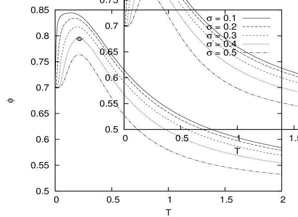
Figure 6: Plot of $\phi$ for a bimodal disorder at constant stress, Eq. (19), with $D_{1}=0$, $D_{2}=1$, $c=0.7$, and a Young modulus $k=1$.

In Fig. 5, we draw equilibrium values of $\chi$ and $\phi$ for $c=0.7$ and applied stress $\sigma=0.3$. It is interesting to see that there are two distinct values of $\chi$ for each value of $\phi$, corresponding to different temperatures. This implies that there are two different microscopic states at each point of the load curve $(\sigma,\epsilon)$. The turning point around $T=0.1$ corresponds to the extremum of $\phi$ in Fig. 6. Figure 7 reports the dependence of $\phi$ on $\sigma$ for different temperatures. In the next Section we make some additional comments on these results.

IV.2 Uniform disorder

Let us look at the case of a uniform distribution of dissociation energies in the interval $[a,b]$. Since we can no longer express the free energy in terms of elementary functions, we are forced to resort to some numerical calculations. In Fig. 8, we compare the phase diagrams of the disordered DTFB and the uniform TFB models. The solid line represents the spinodal for the Helmholtz free energy. In the DTFB model, the averages are taken with respect to two different uniform distributions. It is seen that the main effect of disorder is the weakening of the system at low temperature. In the case of wider distributions of disorder, the spinodal displays a plateau as $T\rightarrow 0$, implying a constant failure stress in that region. For temperature larger than $1$, the TFB and the DTFB models display identical behavior, and the disorder does not affect the system.

V The Edwards-Anderson parameter

In the absence of disorder we may take $\phi$ as the only order parameter of the system. We may replace the ensemble average of a quantity $\langle A\rangle$ by a time average $\lim_{T\rightarrow\infty}1/T\,\int A(t)dt$, and thus interpret the average fraction of intact fibers as the average fraction of time during which a fiber remains intact, corresponding to the thermal average $\langle t_{i}\rangle_{T}$. This is the same for all the fibers since all of them are identical. If disorder is introduced, and the dissociation energy of each fiber becomes different, this no longer holds. The thermal average may be different for each fiber, depending on the value of $D$. Thus, the same macroscopic state, $\phi$, may correspond to different microscopic states, and it might be interesting to distinguish among them, even for practical purposes. A quantity which can operate this distinction is an analog of the Edwards-Anderson parameter Edwards and Anderson (1975),

$$q=\langle\langle t_{i}\rangle_{T}^{2}\rangle.$$

At constant strain, we can write

$$q(\varepsilon,T)=\int dDp(D)\frac{1}{\left[1+\exp\left(\frac{1}{2}\beta k\varepsilon^{2}-\beta D\right)\right]^{2}},$$ (32)

from which it follows that

$$\lim_{T\rightarrow\infty}q=\lim_{T\rightarrow\infty}\phi^{2}=\frac{1}{4},$$

as it could have been anticipated. Then, it seems useful to introduce the quantity $r=q-\phi^{2}$ as a measure of the degree of “freezing” of the system.

Figure 9 shows a detail of the strain stress curve of Fig. 3 for the bimodal distribution at different temperatures. This plot shows that the curves for $T=0.1$ and $T=0.3$ cross at a point in the $(\varepsilon,\sigma)$ plane. This same macroscopic state corresponds to different underlying microscopic states characterized by different values of the elastic modulus $c$. These values can be related to the microscopic state by the analog of the Edwards-Anderson parameter. In fact we have:

$$c=\frac{\partial\sigma}{\partial\epsilon}=k\phi-k\frac{\epsilon^{2}}{T}(\phi-q).$$ (33)

From this expression, together with $\sigma=k\phi\epsilon$, we obtain the values of $\phi$ and $q$. In particular, at the failure, $c=0$, we have

$$q=\frac{\sigma}{k\varepsilon}\left[1-\frac{T}{k\varepsilon^{2}}\right].$$ (34)

Another instance of this lack of uniqueness is given in Figs. 10 a) and b), which have been generated by simulated annealing. The graphs in these figures show the dependence of the “degree of freezing” $r=q-\phi^{2}$ on the applied stress at some low temperature values. The corresponding curves for $\phi$ are given in Figs. 7 a) and b). In analogy with the stress vs strain diagram, the curves for different temperatures cross at some points, where however $r$ assumes distinct values.

VI Conclusions

We have shown that the introduction of disorder in the Thermodynamical Fiber Bundle model Selinger et al. (1991) affects its behavior in many respects. Besides the onset of some expected features, as a decrease in the failure stress at low temperatures, there appear some new features associated with the distribution of disorder. For a bimodal disorder distribution, which leads to an analytically tractable problem, the fraction of integer fibers is non-monotonic in terms of temperature, with an extremum at low temperatures. As a consequence, at either constant stress or constant strain, the system may display the same values of the fraction of integer fibers at different temperatures. However, the corresponding microscopic states are different, which is relevant for understanding delayed fractures, and can be characterized by different values of an analog of the Edwards Anderson parameter.

A.V. is grateful to Fergal Dalton for many useful discussions and suggestions. A.P. S.R.S acknowledge financial support from CNPq and CNR.

Figure 1: Fraction of integer fibers $\phi$ as a function of temperature for different values of the applied strain $\varepsilon$: a), b) in the DTFB model with a uniform distribution of disorder in $[0,2]$; c), d) in the homogeneous TFB model (with no disorder) with $D=1$. For $0.9\approx\varepsilon\approx\sqrt{2}$ these curves differ very little from each other. We always take $k=1$.

Figure 2: Fraction of integer fibers $\phi$ as a function of strain at different temperatures: a) in the DTFB model with a homogeneous distribution of disorder with limits $0$ and $2$; b) in the homogeneous TFB model (no disorder) with $D=1$. We always take $k=1$.

Figure 3: Stress-strain characteristic curves at different temperatures: a) disordered DTFB model with a homogeneous distribution of disorder in $[0,2]$; b) homogeneous TFB model (no disorder) with $D=1$; the case $T=0$ corresponds to the ordinary FB model; c) DTFB model for bimodal disorder, Eq. (19), with parameters $c=0.7$, $D_{1}=0$ and $D_{2}=1$. We always take $k=1$.

Figure 4: Fraction of integer fibers $\phi$ versus temperature $T$ for a bimodal distribution, Eq. (19), with $D_{1}=0$, $D_{2}=1$, $c=0.7$ at constant strain with $k=1$.

Figure 5: Parameters $\chi$ vs $\phi$, after minimization of Eq. (30) and from numerical simulations, in the case of bimodal disorder, Eq. (19), with $c=0.7$ and stress $\sigma=0.3$, from Eq.(30), and $k=1$. It is seen that $\chi$ assumes two different values for the same value of $\phi$.

Figure 7: Stress dependence of $\phi$ at various temperatures for the bimodal distribution of disorder with $D_{1}=0$, $D_{2}=1$, $c=0.7$, and a Young modulus $k=1$.

Figure 8: Comparison between the phase diagram of a case without disorder (TFB with D=1) and the phase diagrams for two homogeneously disordered cases: $D_{i}\in[0.5;1.5]$ and $D_{i}\in[0;2]$. The Young modulus is $k=1$.

Figure 9: A bimodal distribution of disorder with $D_{1}=0$, $D_{2}=1$, $c=0.7$ (we always take $k=1$). It is seen that for two different temperatures, $T=0.1$ and $T=0.3$, stress and strain assume the same values (around $\epsilon=0.35$ and $\sigma=0.28$). The different microscopic configurations can be distinguished by different values of the Edwards-Anderson parameter $q$.

Figure 10: Stress dependence of $r$ at various temperatures for the bimodal distribution of disorder with $D_{1}=0$, $D_{2}=1$, $c=0.7$, and a Young modulus $k=1$. The inset in a) shows that curves for distinct temperatures have distinct values and do not intersect.

References

- Hermann and Roux (1990) H. Hermann and S. Roux, Models for the fracture of disordered media (North Holland, 1990).
- Chakrabarti and Benguigui (1997) B. Chakrabarti and L. G. Benguigui, Statistical physics of fracture and breakdown in disordered systems (Oxford Science Publications, 1997).
- Alava et al. (2006) M. J. Alava, P. K. V. V. Nukala, and S. Zapperi, Advances in Physics 55, 349 (2006).
- Peirce (1926) F. T. Peirce, J. Textile Industry 17, 355 (1926).
- Daniels (1945) H. E. Daniels, Proc. R. Soc. A 183, 405 (1945).
- Hansen and Hemmer (1994) A. Hansen and P. C. Hemmer, Phys. Lett. A 184, 394 (1994).
- Petri et al. (1994) A. Petri, G. Paparo, A. Vespignani, A. Alippi, and M. Costantini, Phys. Rev. Lett. 73, 3423 (1994).
- Caldarelli et al. (1996) G. Caldarelli, F. DiTolla, and A. Petri, Phys. Rev. Lett. 77, 2503 (1996).
- Zapperi et al. (1999) S. Zapperi, P. Ray, H. E. Stanley, and A. Vespignani, Physical Review E 59, 5049 (1999).
- Shahidzadeh-Bonn et al. (2005) N. Shahidzadeh-Bonn, P. Vie , X. Chateau, J.-N. Roux, and D. Bonn, Phys. Rev. Lett. 95, 175501 (2005).
- Golubović and Feng (1991) L. Golubović and S. Feng, Physical Review A 43, 5223 (1991).
- Pauchard and Meunier (1993) L. Pauchard and J. Meunier, Phys. Rev. Lett. 70, 3565 (1993).
- Kitamura et al. (1997) K. Kitamura, I. Maksimov, and K. Nishioka, Philosophical Magazine Letters 75, 343 (1997).
- Maksimov et al. (2001) I. Maksimov, K. Kitamura, and K. Nishioka, Philosophical Magazine Letters 81, 547 (2001).
- Bonn et al. (1998) D. Bonn, H. Kellay, M. Prochnow, K. Ben-Djemiaa, and J. Meunier, Science 280, 265 (1998).
- Politi et al. (2002) A. Politi, S. Ciliberto, and R. Scorretti, Physical Review E 66, 026107 (2002).
- Santucci et al. (2003) S. Santucci, L. Vanel, A. Guarino, R. Scorretti, and S. Ciliberto, Europhys. Lett. 62, 320 (2003).
- Santucci et al. (2004) S. Santucci, L. Vanel, and S. Ciliberto, Physical Review Letters 93, 95505 (2004).
- Sornette and Ouillon (2005) D. Sornette and G. Ouillon, Physical Review Letters 94, 038501 (2005).
- Selinger et al. (1991) R. L. B. Selinger, Z.-G. Wang, W. M. Gelbart, and A. Ben-Shaul, Phys. Rev. A. 43, 4396 (1991).
- Brenner (1962) S. S. Brenner, Journal of Applied Physics 33, 33 (1962).
- (22) A. Virgilii, A. Petri, and S. R. Salinas, in preparation.
- Edwards and Anderson (1975) S. Edwards and P. Anderson, J. Phys. F: Metal Phys. p. 965 (1975).