Boundary multifractality in critical 1D systems with long-range hopping

Abstract

Boundary multifractality of electronic wave functions is studied analytically and numerically for the power-law random banded matrix (PRBM) model, describing a critical one-dimensional system with long-range hopping. The peculiarity of the Anderson localization transition in this model is the existence of a line of fixed points describing the critical system in the bulk. We demonstrate that the boundary critical theory of the PRBM model is not uniquely determined by the bulk properties. Instead, the boundary criticality is controlled by an additional parameter characterizing the hopping amplitudes of particles reflected by the boundary.

I Introduction

Although almost half a century has passed after Anderson’s seminal paper anderson58 , the properties of disordered systems at Anderson localization transitions remain a subject of active current research. This interest is additionally motivated by the understanding that, besides the “conventional” Anderson transition in $d>2$ dimensions, disordered fermions in two dimensions (2D) possess a rich variety of critical points governing quantum phase transitions in these systems.

One of the striking peculiarities of the Anderson transitions is the multifractality of the electronic wave functions Wegner80 ; Castellani-Peliti-86 , see Refs. janssen, ; review, for recent reviews. Specifically, the scaling of moments of the wave functions with the system size $L$ is characterized by a continuum of independent critical exponents $\tau_{q}$,

$$L^{d}\langle|\psi({\bf r})|^{2q}\rangle \sim L^{-\tau_{q}}, \tau_{q} \equiv d(q-1)+\Delta_{q},$$ (1)

where $\langle\ldots\rangle$ denotes the disorder average. In the field-theoretical ($\sigma$-model) language,Wegner80 $\tau_{q}$ are scaling dimensions of higher-order operators describing the moments of the local density of states. Note that one often introduces fractal dimensions $D_{q}$ via $\tau_{q}=D_{q}(q-1)$. In a metal $D_{q}=d$, while at a critical point $D_{q}$ is a nontrivial function of $q$, implying the multifractality of wave functions. Nonvanishing anomalous dimensions $\Delta_{q}\equiv(q-1)(D_{q}-d)$ distinguish a critical point from a metallic phase and determine the scaling of wave function correlations. Among them, $\Delta_{2}<0$ plays the most prominent role, governing the spatial correlations of the intensity $|\psi|^{2}$,

$$L^{2d}\langle|\psi^{2}({\bf r})\psi^{2}({\bf r}^{\prime})|\rangle\sim(|{\bf r}-{\bf r}^{\prime}|/L)^{\Delta_{2}}.$$ (2)

This equation, which in technical terms results from an operator product expansion of the field theory duplantier91 , can be obtained from (1) by using the fact that the wave function amplitudes become essentially uncorrelated at $|{\bf r}-{\bf r}^{\prime}|\sim L$. Scaling behavior of higher order spatial correlations, $\langle|\psi^{2q_{1}}({\bf r}_{1})\psi^{2q_{2}}({\bf r}_{2})\ldots\psi^{2q_{n}}({\bf r}_{n})|\rangle$, can be found in a similar way. Above, the points ${\bf r}_{i}$ were assumed to lie in the bulk of a critical system. In this case we denote the multifractal exponents by $\tau_{q}^{\rm b}$, $\Delta_{q}^{\rm b}$, etc. The multifractality of wave functions has been studied analytically and numerically for a variety of systems: Anderson transition in $d=2+\epsilon$, 3, and 4 dimensions Wegner80 ; akl ; MF-Anderson-numerics , as well as weak multifractality MF-weak , Dirac fermions in random gauge fields MF-Dirac , symplectic-class Anderson transition MF-symplectic , integer quantum Hall MF-IQH and spin quantum Hall Mirlin03 transitions in two dimensions, and power-law random banded matrices MF-RBM .

Recently, the concept of the wave function multifractality was extended subramaniam06 to the surface of a system at the critical point of an Anderson transition. It was shown that the fluctuations of critical wave functions at the surface are characterized by a new set of exponent $\tau_{q}^{\rm s}$ (or, equivalently, anomalous exponents $\Delta_{q}^{\rm s})$, which are in general independent from their bulk counterparts. This boundary critical behavior was explicitly studied, analytically as well as numerically, for the 2D spin quantum Hall transition subramaniam06 ; sqhe-unpub and a 2D weakly localized metal subramaniam06 and, most recently, for the Anderson transition in a 2D system with spin-orbit coupling obuse06 .

In the present paper, we analyze the boundary criticality in the framework of the power-law random banded matrix (PRBM) model prbm ; review ; MF-RBM . The model is defined prbm as the ensemble of random Hermitian matrices $\hat{H}$ (real for $\beta=1$ or complex for $\beta=2$). The matrix elements $H_{ij}$ are independently distributed Gaussian variables with zero mean $\langle H_{ij}\rangle=0$ and the variance

$$\langle|H_{ij}|^{2}\rangle=a^{2}(|i-j|)\ ,$$ (3)

where $a(r)$ is given by

$$a^{2}(r)={1\over 1+(r/b)^{2\alpha}}\ .$$ (4)

At $\alpha=1$ the model undergoes an Anderson transition from the localized ($\alpha>1$) to the delocalized ($\alpha<1$) phase. We concentrate below on the critical value $\alpha=1$, when $a(r)$ falls down as $a(r)\propto 1/r$ at $r\gg b$.

In a straightforward interpretation, the PRBM model describes a 1D sample with random long-range hopping, the hopping amplitude decaying as $1/r^{\alpha}$ with the distance. Also, such an ensemble arises as an effective description in a number of physical contexts (see Ref. MF-RBM, for relevant references). At $\alpha=1$ the PRBM model is critical for arbitrary values of $b$ and shows all the key features of an Anderson critical point, including multifractality of eigenfunctions and nontrivial spectral compressibility prbm ; review . The existence of the parameter $b$ which labels critical points is a distinct feature of the PRBM model: Eq. (3) defines a whole family of critical theories parametrized by $b$. The limit $b\gg 1$ represents a regime of weak multifractality, analogous to the conventional Anderson transition in $d=2+\epsilon$ with $\epsilon\ll 1$. This limit allows for a systematic analytical treatment via the mapping onto a supermatrix $\sigma$-model and the weak-coupling expansion prbm ; review ; MF-RBM . The opposite limit $b\ll 1$ is characterized by very strongly fluctuating eigenfunctions, similarly to the Anderson transition in $d\gg 1$, where the transition takes place in the strong disorder (strong coupling in the field-theoretical language) regime. It is also accessible to an analytical treatment using a real-space renormalization-group (RG) method MF-RBM introduced earlier for related models in Ref. levitov90, .

In addition to the feasibility of the systematic analytical treatment of both the weak-coupling and strong-coupling regimes, the PRBM model is very well suited for direct numerical simulations in a broad range of couplings. For these reasons, it has attracted a considerable interest in the last few years as a model for the investigation of various properties of the Anderson critical point MF-RBM ; prbm-papers . We thus employ the PRBM model for the analysis of the boundary multifractality in this work. The existence of a line of fixed points describing the critical system in the bulk makes this problem particularly interesting. We will demonstrate that the boundary critical theory of the PRBM model is not uniquely determined by the bulk properties. Instead, the boundary criticality is controlled by an additional parameter characterizing the hopping amplitudes of particles reflected by the boundary.

The structure of the paper is as follows. In Sec. II we formulate the model. Section III is devoted to the analytical study of the boundary multifractal spectrum, with the two limits $b\gg 1$ and $b\ll 1$ considered in Secs. III.1 and III.2, respectively. The results of numerical simulations are presented in Sec. IV. Section V summarizes our findings.

II Model

We consider now the critical PRBM model with a boundary at $i=0$, which means that the matrix element $H_{ij}$ is zero whenever one of the indices is negative. The important point is that, for a given value of the bulk parameter $b$, the implementation of the boundary is not unique, and that this degree of freedom will affect the boundary criticality. Specifically, we should specify what happens with a particle which “attempts to hop” from a site $i\geq 0$ to a site $j<0$, which is not allowed due to the boundary. One possibility is that such hops are simply discarded, so that the matrix element variance is simply given by $\langle|H_{ij}|^{2}\rangle=[1+(i-j)^{2}/b^{2}]^{-1}$ for $i,j\geq 0$. More generally, the particle may be reflected by the boundary with certain probability $p$ and “land” on the site $-j>0$. This leads us to the following formulation of the model:

$$\langle|H_{ij}|^{2}\rangle=J_{ij}\ ,$$ (6)

$$J_{ij}=\dfrac{1}{1+\left|i-j\right|^{2}/b^{2}}+\dfrac{p}{1+\left|i+j\right|^{2}/b^{2}}.$$

While the above probability interpretation restricts $p$ to the interval $[0,1]$, the model is defined for all $p$ in the range $-1<p<\infty$. The newly introduced parameter $p$ is immaterial in the bulk, where $i,j\gg|i-j|$ and the second term in Eq. (6) can be neglected. Therefore, the bulk exponents $\tau_{q}^{\rm b}$ depend on $b$ only (and not on $p$), and their analysis performed in Ref. MF-RBM, remains applicable without changes. On the other hand, as we show below by both analytical and numerical means, the surface exponents $\tau_{q}^{\rm s}$ are a function of two parameters, $b$ and $p$.

Equation (6) describes a semi-infinite system with one boundary at $i=0$. For a finite system of a length $L$ (implying that the relevant coordinates are restricted to $0\leq i,j\leq L$) another boundary term, $p^{\prime}/[1+(i+j-2L)^{2}/b^{2}]$, is to be included on the right-hand side of Eq. (6). In general, the parameter $p^{\prime}$ of this term may be different from $p$. This term, however, will not affect the boundary criticality at the $i=0$ boundary, so we discard it below.

III Boundary mutlifractality: Analytical methods

III.1 $b\gg 1$

The regime of weak criticality, $b\gg 1$, can be studied via a mapping onto the supermatrix $\sigma$-model prbm ; review ; MF-RBM , in analogy with the conventional random banded matrix model fyodorov94 . The $\sigma$-model action has the form

$$S[Q]={\beta\over 4}\text{Str}\left[(\pi\nu)^{2}\sum_{i,j=0}^{\infty}J_{ij}Q_{i}Q_{j}-i\pi\nu\omega\sum_{i=0}^{\infty}Q_{i}\Lambda\right],$$ (7)

where $Q_{r}$ is a $4\times 4$ ($\beta=2$) or $8\times 8$ ($\beta=1$) supermatrix field constrained by $Q^{2}_{r}=1$, $\Lambda={\rm diag}({\bf 1},-{\bf 1})$, and Str denotes the supertrace.efetov-book Furthermore, $J_{ij}$ are given by Eq. (6), $\omega$ is the frequency, and $\nu$ is the density of states given by the Wigner semicircle law

$$\nu(E)={1\over 2\pi^{2}b}(4\pi b-E^{2})^{1/2}\ ,\qquad|E|<2\sqrt{\pi b}.$$ (8)

For definiteness, we will restrict ourselves to the band center, $E=0$, below.

To calculate the multifractal spectrum to the leading order in $1/b\ll 1$, we will need the quadratic form of the action (7) expressed in terms of independent coordinates. Parametrizing the field $Q$ (constrained to $Q^{2}=1$) in the usual way,

$$Q_{i}=\Lambda\left(1+W_{i}+\frac{W_{i}^{2}}{2}+\ldots\right),$$ (9)

we obtain the action to the second order in the $W$ fields,

$$S[W]={\pi\nu\beta\over 4}\text{Str}\sum_{i,j=0}^{\infty}W_{i}\left[2\pi\nu(J_{0}^{(i)}\delta_{ij}-J_{ij})-i\omega\delta_{ij}\right]W_{j},$$ (10)

where

$$J_{0}^{(i)}=\sum_{k=0}^{\infty}J_{ik}.$$ (11)

The equation of motion for this action reads (after the Fourier transformation from the frequency into the time domain)

$$\frac{\partial W_{i}(t)}{\partial t}+\pi\nu\sum_{j=0}^{\infty}\left[\delta_{ij}J_{0}^{(i)}-J_{ij}\right]W_{j}(t)=0.$$ (12)

This equation is the analog of the diffusion equation for a metallic system.

The $\sigma$-model action allows us to calculate the moments $\langle|\psi^{2}_{r}|^{q}\rangle$ at a given point $r$. On the perturbative level, the result reads fyodorov94 ; prbm ; review ; MF-RBM

$$\langle|\psi^{2}_{r}|^{q}\rangle={\langle|\psi^{2}_{r}|^{q}\rangle}_{\rm RMT}\left[1+{1\over\beta}q(q-1)\Pi_{rr}\right].$$ (13)

Here the factor ${\langle|\psi^{2}_{r}|^{q}\rangle}_{\rm RMT}$ is the random-matrix-theory result equal to $(2q-1)!!L^{-q}$ for $\beta=1$ and $q!L^{-q}$ for $\beta=2$. The second term in the square brackets in Eq. (13), which constitutes the leading perturbative correction, is governed by the return probability $\Pi_{rr}$ to the point $r$, i.e., the diagonal matrix element of the generalized diffusion propagator $\Pi_{rr^{\prime}}$. The latter is obtained by the inversion of the kinetic operator of Eqs. (10), (12),

$$\pi\nu\sum_{j=0}^{\infty}\left[\delta_{ij}J_{0}^{(i)}-J_{ij}\right]\Pi_{jm}=\delta_{im}-L^{-1}.$$ (14)

(The “diffusion” operator has a zero mode related to the particle conservation. The term $L^{-1}$ on the right-hand side of Eq. (14) ensures that the inversion is taken on the subspace of nonzero modes.) In the bulk case, the inversion is easily performed via the Fourier transform,

$$\Pi_{rr^{\prime}}\longrightarrow\tilde{\Pi}(k)={t\over 8|k|},\qquad|k|\ll b^{-1},$$ (15)

with $t^{-1}={\pi\over 4}(\pi\nu)^{2}b^{2}$, i.e. $t=4/b$ at the band center. The $1/|k|$ behavior of the propagator should be contrasted to its $1/k^{2}$ scaling for a conventional metallic (diffusive) system. This implies that the kinetics governed by Eq. (12) is superdiffusive, also known as Lévy flights levy-flights . Substitution of (15) in Eq. (13) yields a logarithmic correction to the moments of the wave function amplitude,

$$\langle|\psi^{2}_{r}|^{q}\rangle={\langle|\psi^{2}_{r}|^{q}\rangle}_{\rm RMT}\left[1+{q(q-1)\over 2\pi\beta b}\ln{L\over b}\right].$$ (16)

Equation (16) is valid as long as the relative correction is small. The logarithmic divergence of the return probability in the limit $L\to\infty$, which is a signature of criticality, makes the perturbative calculation insufficient for large enough $L$. The problem can be solved then by using the renormalization group (RG), prbm ; review ; MF-RBM which leads to the exponentiation of the perturbative correction in Eq. (16). This results in Eq. (1) with the bulk multifractal exponents

$$\tau_{q}^{\rm b}=(q-1)\left(1-{q\over 2\pi\beta b}\right).$$ (17)

The first term (unity) in the second factor in Eq. (17) corresponds to the normal (metallic) scaling, the second one determines the anomalous exponents

$$\Delta_{q}^{\rm b}={q(1-q)\over 2\pi\beta b}.$$ (18)

At the boundary, the behavior is qualitatively the same: the return probability $\Pi_{rr}$ increases logarithmically with the system size $L$, in view of criticality. However, as we show below, the corresponding prefactor [and thus the prefactor in front of the second term in square brackets in Eq. (16)] is different. After the application of the RG this prefactor emerges in the anomalous exponent,

$$\Delta_{q}^{\rm s}={q(1-q)\over 2\pi\beta b}R_{p}\equiv\Delta_{q}^{\rm b}R_{p}.$$ (19)

In the presence of a boundary the system is not translationally invariant anymore, which poses an obstacle for an analytical calculation of the return probability $\Pi_{rr}$. While for Lévy-flight models with absorbing boundary (that is obtained from our equation (12) with $p=0$ by a replacement of $J_{0}^{(i)}$ with its bulk value $J_{0}$) an analytical progress can be achieved via the Wiener-Hopf method zumofen95 , it is not applicable in the present case, since the kernel of Eq. (12) is not a function of $i-j$ only. We thus proceeded by solving the classical evolution equation (12) numerically with the initial condition $W_{i}(0)=\delta_{ir}$. The value $W_{r}(t)$ of the solution at the point $r$ (i.e. the probability to find the particle at the initial point) decays with the time as $1/t$, so that the integral $\int dtW_{r}(t)$ yields the logarithmically divergent return probability discussed above. Extracting the corresponding prefactor, we find the anomalous exponent,

$${\Delta_{q}\over q(1-q)}={1\over\beta}tW_{r}(t)|_{t\to\infty}.$$ (20)

Note that the limit of the large system size $L\to\infty$ should be taken in Eq. (20) before $t\to\infty$, so that the particle does not reach the boundary for $r$ in the bulk (or, for $r$ at the boundary, does not reach the opposite boundary).

We have checked that the numerical implementation of Eqs. (20), (12) reproduces the analytical result (18) in the bulk. We then proceeded with numerical evaluation of the surface multifractal exponents $\Delta_{q}^{\rm s}$. For this purpose, we have discretized the time variable in Eq. (12) with a step $\Delta t=1/2$. With the parameters $\pi\nu=1/\pi$, $b=10$, $L=10000$, and $t=500$, the product $tW_{r}(t)$ yields its required asymptotic value with the accuracy of the order of $2\%$. The results for the corresponding prefactor $R_{p}$, as defined in Eq. (19), are shown in Fig. 1 for several values of $p$ between 0 and 3. It is seen that the boundary exponents not only differ from their bulk counterparts but also depend on $p$.

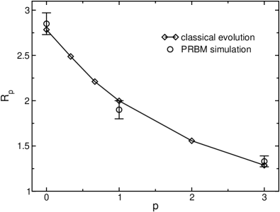
Figure 1: The ratio $R_{p}=\Delta_{q}^{\rm s}(b,p)/\Delta_{q}^{\rm b}(b)$ of the surface and bulk anomalous exponents for large $b$, as a function of the reflection parameter $p$. Diamonds represent the results of the $\sigma$-model analysis with a numerical solution of the corresponding classical evolution equation, as described in Sec. III.1. Circles represent a direct computer simulation of the PRBM model, Eqs. (6), (6), see Sec. IV, with $b=8$. The ratio $R_{p}$ has been evaluated for the range $0<q<1$, where the numerical accuracy of the anomalous exponents is the best. Within this interval we find that $R_{p}$ is $q$-independent (within numerical errors) in agreement with Eq. (19).

For the particular case of the reflection probability $p=1$ we can solve the evolution equation (12) and find $\Delta_{q}^{\rm s}$ analytically. Indeed, the corresponding equation can be obtained from its bulk counterpart (defined on the whole axis, $-\infty<i<\infty$) by “folding the system” on the semiaxis $i>0$ according to $W_{i}(t)+W_{-i}(t)\longrightarrow W_{i}(t)$, cf. Ref. levy-p1, . This clearly leads to a doubling of the return probability, so that

$$R_{1}=2,$$ (21)

in full agreement with the numerical solution of the evolution equation.

III.2 $b\ll 1$

In the regime of small $b$ the eigenstates are very sparse. In this situation, the problem can be studied by a real-space RG method that was developed in Ref. levitov90, for related models and in Ref. MF-RBM, for the PRBM model. Within this approach, one starts from the diagonal part of the Hamiltonian and then consecutively includes into consideration nondiagonal matrix elements $H_{ij}$ with increasing distance $\rho=|i-j|$. The central idea is that only rare events of resonances between pairs of remote states are important, and that there is an exponential hierarchy of scales at which any given state finds a resonance partner: $\ln\rho_{1}\sim b^{-1}$,   $\ln\rho_{2}\sim b^{-2}$, …. This allows one to formulate RG equations for evolution of quantities of interest with the “RG time” $t=\ln\rho$. We refer the reader for technical details of the derivation to Ref. MF-RBM, where the evolution equation of the distribution $f(P_{q})$ of the inverse participation ratios, $P_{q}=\sum_{r}|\psi_{r}^{2}|^{q}$, as well as of the energy level correlation function, was derived. In the present case, we are interested in the statistics of the local quantity, the wave function intensity $|\psi_{r}^{2}|$ at a certain point $r$. Assuming first that $r$ is in the bulk and generalizing the derivation of Ref. MF-RBM, , we get the evolution equation for the corresponding distribution function $f(y\equiv|\psi_{r}^{2}|)$,

$${\partial f(y,\rho)\over\partial\ln\rho} = {2b\over\pi}\int_{0}^{\pi/2}{d\theta\over\sin^{2}\theta\cos^{2}\theta}\int_{-\infty}^{\infty}dy^{\prime}f(y^{\prime},\rho)$$ (22)

$$\times [\delta(y-y^{\prime}\cos^{2}\theta)+\delta(y-y^{\prime}\sin^{2}\theta)$$

$$-\delta(y-y^{\prime})-\delta(y)].$$

Equation (22) is written for $\beta=1$; in the case of $\beta=2$ one should make a replacement $b\longrightarrow(\pi/2\sqrt{2})b$. The physical meaning of Eq. (22) is rather transparent: its right-hand side is a “collision integral” describing a resonant mixture of two states with the intensities $y^{\prime}$ and $0$ at the point $r$, leading to formation of superposition states with the intensities $y^{\prime}\cos^{2}\theta$ and $y^{\prime}\sin^{2}\theta$. Multiplying Eq. (22) by $y^{q}$ and integrating over $y$, we get the evolution equation for the moments $\langle y^{q}\rangle$,

$${\partial\langle y^{q}\rangle\over\partial\ln\rho}=-2bT(q)\langle y^{q}\rangle\ ,$$ (23)

where

$$T(q) = {1\over\pi}\int_{0}^{\pi/2}{d\theta\over\sin^{2}\theta\cos^{2}\theta}(1-\cos^{2q}\theta-\sin^{2q}\theta)$$ (24)

$$= {1\over 2^{2q-3}}{\Gamma(2q-1)\over\Gamma(q)\Gamma(q-1)}.$$

The RG should be run until $\rho$ reaches the system size $L$. Thus, the bulk multifractal exponents are equal to

$$\tau_{q}^{b}=2bT(q),$$ (25)

in agreement with Ref. MF-RBM, .

How will the evolution equation (22) be modified if the point $r$ is located at the boundary? First, the factor 2 on the right-hand side of (22) will be absent. Indeed, this factor originated from the probability to encounter a resonance. In the bulk, the resonance partner can be found either to the left or to the right, thus the factor of two. For a state at the boundary only one of these possibilities remains, so this factor is absent. Second, one should now take into account also the second term in the variance $J_{ij}$ of the matrix element $H_{ij}$, Eq. (6). In view of the hierarchy of resonances described above, the relevant matrix elements will always connect two points, one of which is much closer to the boundary than the other (say, $i\ll j$). In this situation, the two terms in (6) become equivalent (up to the prefactor $p$ in the second term) and can be combined,

$$J_{ij}\simeq{(1+p)b^{2}\over j^{2}}\ ,\qquad i\ll j.$$ (26)

Therefore, the effect of the second term amounts to the rescaling $b\longrightarrow(1+p)^{1/2}b$. Combining both the effects, we get the boundary multifractal exponents,

$$\tau_{q}^{\rm s}=(1+p)^{1/2}bT(q)={(1+p)^{1/2}\over 2}\tau_{q}^{\rm b}.$$ (27)

The above real-space RG method works for $q>1/2$, where the multifractal exponent $\tau_{q}$ is small note1 . The results can, however be extended to the range of $q<1/2$ by using the recently found symmetry relation between the multifractal exponents mirlin06 ,

$$\Delta_{q}=\Delta_{1-q}.$$ (28)

Independently of whether $q$ is larger or smaller than 1/2, the obtained relation between the surface and the bulk multifractal spectra can be formulated in the following way:

$$\tau_{q}^{\rm s}(b,p)=\tau_{q}^{\rm b}(b\longrightarrow b(1+p)^{1/2}/2).$$ (29)

IV Boundary multifractality: Numerical simulations

In this section we present the results for the multifractality spectra obtained by direct numerical simulations of the PRBM model, Eqs. (6), (6), with $\beta=1$. The model has been implemented with two boundaries, each one having the same boundary parameter $p$. Using standard diagonalization routines, systems with sizes $L=128,\,256,\,512,\,1024,\,2048$ and $4096$ sites have been studied with ensembles comprising of $10^{7}$ ($L=128$, $3\cdot 10^{8}$ wave functions) to $5000$ ($L=4096$, $5\cdot 10^{6}$ wave functions) disorder configurations. The multifractal analysis has been performed with intensities $|\psi_{r}^{2}|$ averaged (coarse grained) over blocks of four neighboring sites in order to access negative $q$ values, $q\gtrsim-2$. For the analysis of the surface multifractal exponents, only the four sites closest to boundaries have been taken into account.

Figure 2 illustrates nicely our main findings. We show there the dependence of the anomalous dimension $\Delta_{2}\equiv D_{2}-1$ on $b$ in the bulk and at the boundary, for three different values of the reflection parameter $p$. It is seen, first of all, that the bulk exponent $\Delta_{2}^{b}$ does not depend on $p$, in agreement with the theory. Second, the boundary exponent $\Delta_{2}^{s}$ is different from the bulk one. Third, the boundary exponent is not determined by $b$ only, but rather depends on the boundary parameter $p$ as well. The lower panel of Fig. 2 demonstrates the agreement between the numerical results and the analytical asymptotics of small and large $b$.

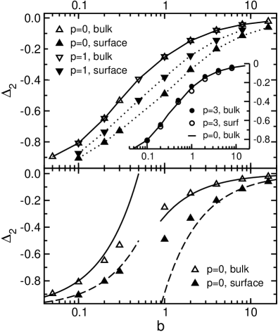
Figure 2: Upper panel: Anomalous exponent $\Delta_{2}\equiv D_{2}-1$ as a function of $b$ from numerical simulations in the bulk and at the boundary for the reflection parameter $p=0$ and $1$. The inset shows data for $p=3$ compared to the $p=0$ bulk values. Lower panel: Surface and bulk data for $p=0$ compared with analytical results for small and large $b$ (using $R_{0}=2.78$), Eqs. (18), (19), (25), (27).

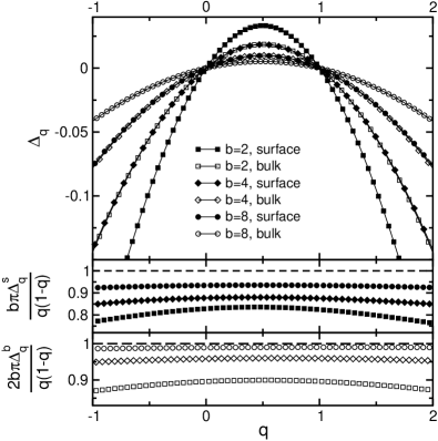
Figure 3: Upper panel: Boundary and bulk multifractal spectra, $\Delta_{q}^{\rm s}$ and $\Delta_{q}^{\rm b}$, at $b=2$, $4$, and $8$ for the reflection parameter $p=1$. In accordance with Eq. (21), the surface multifractality spectrum is enhanced by a factor close to two compared to the bulk.
Middle panel: Surface spectrum divided by the analytical large-$b$ result, Eq. (19). The dashed line represents the analytical result for $b\gg 1$. With increasing $b$, the numerical data nicely converges towards the analytical result.
Lower panel: Analogous plot for the bulk spectrum, Eq. (18). The error estimate from the finite size extrapolation is $3\%$.

Having discussed the $b$-dependence of the fractal exponent with fixed $q$ (equal to 2) shown in Fig. 2, we turn to Fig. 3, where the whole multifractal spectra $\Delta_{q}$ are shown for fixed large values of $b$. Specifically, the anomalous dimensions $\Delta_{q}^{\rm s}$ and $\Delta_{q}^{\rm b}$ are presented for $b=2,\,4$, and 8, with the reflection parameter chosen to be $p=1$. For all curves the $q$ dependence is approximately parabolic, as predicted by the large-$b$ theory, Eqs. (18) and (19), with the prefactor inversely proportional to $b$. To clearly demonstrate this, we plot in the lower two panels the exponents $\Delta_{q}$ divided by the corresponding analytical results of the large-$b$ limit. While for moderately large $b$ the ratio shows some curvature, the latter disappears with increasing $b$ and the ratio approaches unity, thus demonstrating the full agreement between the numerical simulations and the analytical predictions. It is also seen in Fig. 3 that the bulk multifractality spectrum for $b=4$ and the surface spectrum for $b=8$ are almost identical, in agreement with Eq. (21). The same is true for the relation between the bulk spectrum for $b=2$ and the surface spectrum for $b=4$.

We have further calculated the ratio of the large-$b$ surface and bulk anomalous dimensions, $R_{p}=\Delta_{q}^{\rm s}/\Delta_{q}^{\rm b}$, for several values of the reflection parameter, $p=0$, 1, and 3. As shown in Fig. 1, the results are in good agreement with the $\sigma$-model predictions for $R_{p}$ obtained in Sec. III.1.

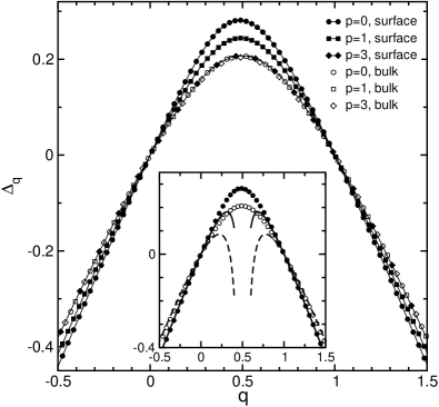
Figure 4: Main panel: Numerically determined boundary and bulk anomalous dimensions $\Delta_{q}$ at $b=0.1$ for $p=0$, $1$, and $3$. As expected, the bulk anomalous dimension is independent of the value of $p$. In accordance with Eq. (29), for $p=3$ surface and bulk dimensions have the same values.
Inset: The $p=0$ data compared to the analytical results, surface [solid line, Eq. (27)] and bulk [dashed line, Eq. (25)]. Analytical data have been calculated for $q\geq 0.6$ and mirrored for $q\leq 0.4$ by using the symmetry relation $\Delta_{q}=\Delta_{1-q}$. Note that the analytical result (25) breaks down in the vicinity of $q=1/2$, at $|q-1/2|\lesssim 1/\ln b^{-1}$, see Ref. note1, . At the boundary, one should replace $b\to b(1+p)^{1/2}/2$ in this condition. We see, indeed, that for $b=0.1$, $p=0$ the analytical formula works up to $|q-1/2|\simeq 0.4$ in the bulk and $|q-1/2|\simeq 0.3$ at the boundary.

In Fig. 4 the surface and bulk multifractal spectra are shown for the case of small $b$. While the spectra are strongly nonparabolic in this limit, they clearly exhibit the symmetry $q\to 1-q$, Eq. (28). The data are in good agreement with the RG results of Sec. III.2. In particular, the surface spectrum for $p=3$ is essentially identical to the bulk spectrum, as predicted by Eq. (29). In the inset, the surface and bulk multifractality spectra for $p=0$ are compared with the analytical asymptotics, Eqs. (25), (27), supplemented by the symmetry relation (28). Again, a very good agreement is seen, except for a vicinity of $q=1/2$, where Eqs. (25), (27) break down.note1

V Conclusions

In summary, we have studied the boundary multifractality of wave functions in the PRBM model describing a critical 1D system with long-range hopping. Our findings strongly corroborate the ubiquity of the notion of boundary mutlifractality (recently introduced in Ref. subramaniam06, ) in the context of disordered electronic systems at criticality. We have demonstrated, both analytically and numerically, that the surface multifractal exponents $\tau_{q}^{\rm s}(b,p)$ are not only different from their bulk counterparts, $\tau_{q}^{\rm b}(b)$, but also depend on an additional parameter $p$ characterizing the reflection of the particle at the boundary. This peculiarity of the PRBM model is intimately related to the existence of the line of fixed points (labelled by $b$) in the bulk model. Indeed, the freedom in the choice of the amplitude of the boundary “hopping with reflection” term is of the same origin as the freedom in the amplitude of the power-law hopping in the bulk.

We close on a somewhat speculative note. The existence of a truly marginal coupling (implying a line of fixed points) is not unique for the PRBM model. In particular, the 2D Dirac fermions in a random vector potential MF-Dirac share this feature. Furthermore, it was conjectured recently CFT-IQH-Zirnbauer ; CFT-IQH-Tsvelik that the quantum Hall transition might be described by a particular point on a line of fixed points in a related model. Based on our results, it is natural to ask whether the emergence of an additional parameter $p$ governing the boundary criticality is a general property of critical theories with a truly marginal coupling. The work in this direction is currently underway unpub .

VI Acknowledgments

The work of AM, RN, FE, and ADM was supported by the Center for Functional Nanostructures and the Schwerpunktprogramm “Quanten-Hall-Systeme” of the Deutsche Forschungsgemeinschaft. The work of IAG and ARS was supported by the NSF MRSEC Program under DMR-0213745, the NSF Career Award DMR-0448820, the Sloan Research Fellowship from Alfred P Sloan Foundation and the Research Innovation Award from Research Corporation. ARS, IAG, and ADM acknowledge hospitality of the Kavli Institute for Theoretical Physics at Santa Barbara and support by the National Science Foundation under Grant No. PHY99-07949.

References

- (1) Also at Petersburg Nuclear Physics Institute, 188300 St. Petersburg, Russia.
- (2) P. W. Anderson, Phys. Rev. 109, 1492 (1958).
- (3) F. Wegner, Z. Phys. B 36, 209 (1980).
- (4) C. Castellani and L. Peliti, J. Phys. A 19, L429 (1986).
- (5) M. Janssen, Phys. Rep. 295, 1 (1998).
- (6) A. D. Mirlin, Phys. Rep. 326, 259 (2000).
- (7) B. Duplantier and A. W. W. Ludwig, Phys. Rev. Lett. 66, 247 (1991).
- (8) B. L. Altshuler, V. E. Kravtsov, and I. V. Lerner, Sov. Phys. JETP 64, 1352 (1986).
- (9) M. Schreiber and H. Grussbach, Phys. Rev. Lett. 67, 607 (1991); A. Mildenberger, F. Evers, and A. D. Mirlin, Phys. Rev. B 66, 033109 (2002).
- (10) V. I. Fal’ko and K. B. Efetov, Europhys. Lett. 32, 627 (1995); Phys. Rev. B 52, 17 413 (1995).
- (11) A. W. W. Ludwig, M. P. A. Fisher, R. Shankar, and G. Grinstein, Phys. Rev. B 50, 7526 (1994); C. Mudry, C. Chamon, and X.-G.Wen, Nucl. Phys. B 466, 383 (1996); H. E. Castillo, C. Chamon, E. Fradkin, P. M. Goldbart, and C. Mudry, Phys. Rev. B 56, 10 668 (1997); J.-S. Caux, N. Taniguchi, and A. M. Tsvelik, Nucl. Phys. B 525, 671 (1998); Phys. Rev. Lett. 80, 1276 (1998); J.-S. Caux, Phys. Rev. Lett. 81, 4196 (1998).
- (12) S. N. Evangelou, Physica A 167, 199 (1990); J. T. Chalker, G. J. Daniell, S. N. Evangelou, and I. H. Nahm, J. Phys.: Cond. Matter 5, 485 (1993); L. Schweitzer, J. Phys. C 7, L281 (1995); T. Kawarabayashi and T. Ohtsuki, Phys. Rev. B 53, 6975, (1996); K. Yakubo and M. Ono, Phys. Rev. B 58, 9767 (1998); A. Mildenberger and F. Evers, Phys. Rev. B 75, 041303(R) (2007).
- (13) W. Pook and M. Janssen, Z. Phys. B 82, 295 (1991); B. Huckestein, B. Kramer, and L. Schweitzer, Surf. Sci. 263, 125 (1992); B. Huckestein, Rev. Mod. Phys. 67, 357 (1995); R. Klesse and M. Metzler, Europhys. Lett, 32, 229 (1995); Int. J. Mod. Phys. C 10, 577 (1999); M. Janssen, M. Metzler, and M. R. Zirnbauer, Phys. Rev. B 59, 15 836 (1999); F. Evers, A. Mildenberger, and A. D. Mirlin, Phys. Rev. B 64, 241303(R) (2001).
- (14) A. D. Mirlin, F. Evers, and A. Mildenberger, J. Phys. A 36, 3255 (2003).
- (15) A. D. Mirlin and F. Evers, Phys. Rev. B 62, 7920 (2000).
- (16) A. R. Subramaniam, I. A. Gruzberg, A. W. W. Ludwig, F. Evers, A. Mildenberger, and A. D. Mirlin, Phys. Rev. Lett. 96, 126802 (2006).
- (17) A. R. Subramaniam, I. A. Gruzberg, and A. W. W. Ludwig, to be published.
- (18) H. Obuse, A. R. Subramaniam, A. Furusaki, I. A. Gruzberg, and A. W. W. Ludwig, cond-mat/0609161, accepted in Phys. Rev. Lett.
- (19) A. D. Mirlin, Y. V. Fyodorov, F.-M. Dittes, J. Quezada, and T. H. Seligman, Phys. Rev. E 54, 3221 (1996).
- (20) L. S. Levitov, Phys. Rev. Lett. 64, 547 (1990); B. L. Altshuler and L. S. Levitov, Phys. Rep. 288, 487 (1997).
- (21) V. E. Kravtsov and K. A. Muttalib, Phys. Rev. Lett. 79, 1913 (1997); V. E. Kravtsov and A. M. Tsvelik, Phys. Rev. B 62, 9888 (2000); E. Cuevas, M. Ortuno, V. Gasparian, and A. Perez-Garrido, Phys. Rev. Lett. 88, 016401 (2001); I. Varga, Phys. Rev. B 66, 094201 (2002); E. Cuevas, Phys. Rev. B 68, 024206 (2003); ibid. 68, 184206 (2003); ibid. 71, 024205 (2005); O. Yevtushenko and V. E. Kravtsov, J. Phys. A: Math. Phys. 36, 8265 (2003); Phys. Rev. E 69, 026104 (2004); A. M. Garcia-Garcia and K. Takahashi, Nucl.Phys. B 700, 361 (2004); J. A. Mendez-Bermudez and T. Kottos, Phys. Rev. B 72, 064108 (2005); A. M. Garcia-Garcia, Phys.Rev. E 73 026213 (2006); V. E. Kravtsov, O. Yevtushenko, and E. Cuevas, J. Phys. A: Math. Gen. 39, 2021 (2006). J. A. Mendez-Bermudez and I. Varga, Phys. Rev. B 74, 125114 (2006).
- (22) Y. V. Fyodorov and A. D. Mirlin, Int. J. Mod. Phys. B 8, 3795 (1994).
- (23) For a detailed exposition of the supersymmetry method the reader is referred to the book, K. B. Efetov, Supersymetry in disorder and chaos (Cambridge University Press, 1997).
- (24) M. F. Schlesinger, G. M. Zaslavsky, and J. Klafter, Nature 363, 31 (1993); R. Metzler and J. Klafter, Phys. Rep. 339, 1 (2000).
- (25) G. Zumofen and J. Klafter, Phys. Rev. E 51, 2805 (1995).
- (26) R. Metzler and J. Klafter, Physica A 278, 107 (2000); N. Krepysheva, L. Di Pietro, and M.-C. Néel, Phys. Rev. E 73, 021104 (2006).
- (27) Strictly speaking, Eqs. (25), (24) are valid for all in the limit . For a finite (but small) , Eq. (25) breaks down in a narrow interval of above , namely for . Indeed, the evolution equation (22) assumes that resonances are rare, i.e., that the angle describing the resonant mixture is large compared to its typical, nonresonant, value . On the other hand, when approaches 1/2, the integral in Eq. (24) converges at . Comparing this with , we get the above restriction on the validity of Eq. (25).
- (28) A. D. Mirlin, Y. V. Fyodorov, A. Mildenberger, and F. Evers, Phys. Rev. Lett. 97, 046803 (2006).
- (29) M. R. Zirnbauer, hep-th/9905054.
- (30) M. J. Bhaseen, I. I. Kogan, O. A. Soloviev, N. Taniguchi, and A. M. Tsvelik, Nucl. Phys. B 580, 688 (2000).
- (31) A. R. Subramaniam et al., unpublished.