Perturbation expansion for the diluted two-dimensional $XY$ model

Abstract

We study the quasi-long-range ordered phase of a 2D XY model with quenched site-dilution using the spin-wave approximation and expansion in the parameter which characterizes the deviation from completely homogeneous dilution. The results, obtained by keeping the terms up to the third order in the expansion, show good accordance with Monte Carlo data in a wide range of dilution concentrations far enough from the percolation threshold. We discuss different types of expansion.

The XY model in two dimensions is the simplest example of a system exhibiting “quasi-long-range order” (QLRO), which appears at low temperatures in a number of physical models of great importance, e.g. magnetic films with planar anisotropy, but also thin-film superfluids or superconductors, two-dimensional solids, 2d-classical Coulomb gas or fluctuating surfaces and the roughness transition [2, 3]. Although no exact solution exists for this model, most of its properties are known from different approaches.

Destruction of long range ordering is due to the presence of stable topological defects (vortices) [4, 5, 6], a situation which strongly contrasts with usual ordering in systems undergoing a ferromagnetic phase transition. First, the magnetization of the XY model on an infinite 2D lattice remains zero at any non-zero temperature [7], thus it is impossible to describe in the thermodynamic limit the quasi-long-range ordered phase by this usual order parameter, however the spin-spin pair correlation function gives a distinct indication of QLRO. Its asymptotic behaviour changes from exponential at high temperatures to power low decay at low temperatures. This transition is referred to as the Berezinskii-Kosterlitz-Thouless (BKT) transition and the point where this change of behaviour occurs is the BKT temperature.

A quantity of interest which characterizes the QLRO phase, is then the temperature dependent exponent of the correlation function:

$$\eta(T)=-\lim_{|{\bf R}|\to\infty}\frac{\ln\left<{\bf S_{\bf r}\cdot S_{r+R}}\right>}{\ln|{\bf R}|}.$$ (1)

The spin-wave analysis of the model gives a reliable value of $\eta$ for small enough temperatures [9]. The reliability of the harmonic approximation for this model is grounded by the RG analysis [6].

The case of the (classical) XY model on a regular lattice (without defects)

$$H=-\frac{1}{2}\sum_{\bf r}\sum_{\bf r^{\prime}}J({\bf r-r^{\prime}})\left(S^{x}_{\bf r}S^{x}_{\bf r^{\prime}}+S^{y}_{\bf r}S^{y}_{\bf r^{\prime}}\right),$$ (2)

has been studied intensively (when $J({\bf r-r^{\prime}})$ is limited to nearest neighbours) and its properties are well known (see e.g. Ref. [3]). The addition of defects (site-dilution, bond-dilution) has been considered as a trivial modification, since the Harris criterion [10] states in this case that the universality class of the diluted model remains the same as that of the pure one. It means that the critical exponents of both pure and disordered models are unchanged, when evaluated at their corresponding BKT points, e.g. $\eta^{{\rm dil}}(T^{{\rm dil}}_{BKT})=\eta^{{\rm pure}}(T^{{\rm pure}}_{BKT})$, but the functions $\eta^{{\rm pure}}(T)$ and $\eta^{{\rm dil}}(T)$ characterizing the low temperature phase of pure and disordered systems are different and the exact behaviour of $\eta^{{\rm dil}}(T)$ is a question which deserves attention. For example, it is not obvious how the impurities can interact with the vortices and influence the QLRO. This question is addressed e.g. in Refs. [11, 12].

In a previous paper [13] the influence of uncorrelated (normally distributed) site-dilution was considered and a perturbation expansion for the case of weak dilution was proposed. The two-spin coupling term $J({\bf r-r^{\prime}})$ in Eq. (2) was replaced by $J({\bf r-r^{\prime}})c_{\bf r}c_{\bf r^{\prime}}$ with

$$c_{\bf r}=\left\{\begin{array}[]{ll}1,&\textrm{if the site ${\bf r}$ has a spin;}\\ 0,&\textrm{if the site ${\bf r}$ is empty.}\end{array}\right.$$ (3)

The physical quantities which characterize the system with quenched disorder after the thermodynamical averaging must be averaged over all possible configurations of dilution. This configurational averaging is denoted as $\overline{(...)}$:

$$\overline{(...)}=\prod_{\bf r}\sum_{c_{\bf r}=0,1}[c\delta_{1-c_{\bf r},0}+(1-c)\delta_{c_{\bf r},0}](...),$$ (4)

where $c$ is the concentration of occupied sites.

Starting with the Hamiltonian in the harmonic approximation,

$$H=\frac{1}{4}\sum_{\bf r}\sum_{\bf r^{\prime}}J({\bf r-r^{\prime}})\left(\theta_{\bf r}-\theta_{\bf r^{\prime}}\right)^{2}c_{\bf r}c_{\bf r^{\prime}}\ ,$$ (5)

and realizing the Fourier transformation of the variables:

$$\theta_{\bf r} = \frac{1}{\sqrt{N}}\sum_{\bf k}e^{i{\bf kr}}\theta_{\bf k},\qquad\theta_{\bf k}=\frac{1}{\sqrt{N}}\sum_{\bf r}e^{-i{\bf kr}}\theta_{\bf r},$$ (6)

$$J({\bf r}) = \frac{1}{N}\sum_{\bf q}e^{i{\bf qr}}\nu({\bf q}),\qquad\nu({\bf q})=\sum_{\bf r}e^{-i{\bf qr}}J({\bf r}),$$ (7)

($N$ is the number of sites in the lattice, and ${\bf k}$ runs over the 1st Brillouin zone), one has

$$H = J\sum_{\bf k}\gamma_{\bf k}\theta_{\bf k}\theta_{\bf-k}+J\sum_{\bf k}\sum_{\bf k^{\prime}}(\gamma_{\bf k+k^{\prime}}-\gamma_{\bf k}-\gamma_{\bf k^{\prime}})\rho({\bf k+k^{\prime}})\theta_{\bf k}\theta_{\bf k^{\prime}}$$

$$+ J\sum_{\bf k}\sum_{\bf k^{\prime}}\sum_{\bf q}(2-\gamma_{\bf q})\left[\rho({\bf-k-k^{\prime}-q})\rho({\bf q})-\rho({\bf-k-q})\rho({\bf-k^{\prime}+q})\right]\theta_{\bf k}\theta_{\bf k^{\prime}}$$

where $\rho({\bf q})=\frac{1}{N}\sum_{\bf r}e^{-i{\bf qr}}(1-c_{\bf r})$, and $\gamma_{\bf k}\ \equiv\ \frac{1}{2J}\left[\nu(0)-\nu({\bf k})\right]=2-\cos k_{x}a-\cos k_{y}a$ on the square lattice. The first term is the Hamiltonian of the pure system, so one can consider $\rho$ as a parameter of perturbation of this Hamiltonian. Note, that power of $\rho$ corresponds to the number of sums over ${\bf k}$. A classification of the perturbation theory series with respect to number of sums over ${\bf k}$ corresponds to the expansion in the ratio of the volume of effective interaction to the elementary cell volume [14]. Taking this ratio to be small means that it is valid for the short-range interacting systems, which holds for our problem.

The linear approximation in $\rho$-expansion presented in Ref. [13] gives the result for the exponent of the pair correlation function:

$$\eta^{{\rm dil}}\ =\ \left(1+2(1-c)\right)\eta^{{\rm pure}}+O(\rho^{2}).$$ (9)

Here we can report the result for this expansion up to the second order in $\rho$:

$$\eta^{{\rm dil}}\ =\ \left(1+2.73(1-c)+1.27(1-c)^{2}\right)\eta^{{\rm pure}}+O(\rho^{3}),$$ (10)

The figures follow from numerical estimate of sums. The 1st and 2nd order perturbation expressions fit the Monte Carlo results only for very small concentrations of dilution (see Fig. 1). Unfortunately the calculation of the third order seems to be too tedious and perhaps does not deserve so much effort, therefore it is desirable to investigate another road.

In the present paper we propose to introduce the parameter of expansion in a different manner in order to extend the region of reliability of the expansion to stronger dilutions (but of course still far enough from the percolation threshold where the whole approach fails) and to improve convergence. We will keep the notation $\rho$, but from now on one should understand it as the deviation from homogeneously diluted system:

$$\rho({\bf q})=\frac{1}{N}\sum_{\bf r}e^{-i{\bf qr}}(c_{\bf r}-c).$$ (11)

We did not make any assumption about weakness of disorder, we may thus expect that the results of this expansion will be less sensitive to the value of dilution $c$. Rewriting the Hamiltonian with this new parameter one gets

$$H = c^{2}J\sum_{\bf k}\gamma_{\bf k}\theta_{\bf k}\theta_{\bf-k}-cJ\sum_{\bf k}\sum_{\bf k^{\prime}}(\gamma_{\bf k+k^{\prime}}-\gamma_{\bf k}-\gamma_{\bf k^{\prime}})\rho({\bf k+k^{\prime}})\theta_{\bf k}\theta_{\bf k^{\prime}}$$ (12)

$$+ J\sum_{\bf k}\sum_{\bf k^{\prime}}\sum_{\bf q}(2-\gamma_{\bf q})\left[\rho({\bf-k-k^{\prime}-q})\rho({\bf q})-\rho({\bf-k-q})\rho({\bf-k^{\prime}+q})\right]\theta_{\bf k}\theta_{\bf k^{\prime}}$$

$$\equiv c^{2}H_{{\rm pure}}+H_{\rho}+H_{\rho^{2}}\ ,$$

where the first term is the Hamiltonian of the pure system now with a renormalized coupling.

The spin-spin pair correlation function,

$$G_{2}(R)=\overline{c_{\bf r}c_{\bf r+R}\left<\cos(\theta_{\bf r+R}-\theta_{\bf r})\right>}=\overline{c_{\bf r}c_{\bf r+R}\frac{\left<\cos(\theta_{\bf r+R}-\theta_{\bf r})e^{-\beta(H_{\rho}+H_{\rho^{2}})}\right>_{*}}{\left<e^{-\beta(H_{\rho}+H_{\rho^{2}})}\right>_{*}}}$$ (13)

can be expanded in $\rho$ and then configurationally averaged. In (13), $\left<...\right>_{*}$ stands for the averaging with the pure system Hamiltonian with renormalized coupling $c^{2}J$. Using (4) one has the equalities: $\overline{\rho({\bf q})}\ =\ 0$, $\overline{\rho({\bf q})\rho({\bf q^{\prime}})}\ =\ c(1-c)\frac{1}{N}\delta_{{\bf q+q^{\prime}},0}$ and $\overline{\rho({\bf q})\rho({\bf q^{\prime}})\rho({\bf q^{\prime\prime}})}\ =\ c(1-3c+2c^{2})\frac{1}{N^{2}}\delta_{{\bf q+q^{\prime}+q^{\prime\prime}},0}$, which, inserted into the expansion lead after tedious calculations to the third order expression

$$\overline{c_{\bf r}c_{\bf r+R}\left<\cos(\theta_{\bf r+R}-\theta_{\bf r})\right>}=c^{2}\left<\cos(\theta_{\bf r+R}-\theta_{\bf r})\right>_{*}$$

$$\times\ \Bigg{[}\ \ 1-\frac{1-c}{c^{3}}\frac{1}{\beta JN^{2}}\sum_{{\bf k},{\bf k^{\prime}}}\frac{(\gamma_{{\bf k}+{\bf k^{\prime}}}-\gamma_{{\bf k}}-\gamma_{{\bf k^{\prime}}})^{2}}{\gamma^{2}_{\bf k}\gamma_{\bf k^{\prime}}}\sin^{2}\frac{\bf kR}{2}$$

$$+\frac{1-3c+2c^{2}}{c^{4}}\frac{1}{\beta J}{\textstyle\Bigg{(}\frac{2}{N}\sum_{{\bf k}}\frac{\sin^{2}\frac{\bf kR}{2}}{\gamma_{\bf k}}}$$

$$\textstyle-\frac{1}{N^{3}}\sum_{{\bf k},{\bf k^{\prime}},{\bf k^{\prime\prime}}}\frac{(\gamma_{{\bf k}+{\bf k^{\prime}}}-\gamma_{{\bf k}}-\gamma_{{\bf k^{\prime}}})(\gamma_{{\bf k^{\prime}}-{\bf k^{\prime\prime}}}-\gamma_{{\bf k^{\prime}}}-\gamma_{{\bf k^{\prime\prime}}})(\gamma_{{\bf k}+{\bf k^{\prime\prime}}}-\gamma_{{\bf k}}-\gamma_{{\bf k^{\prime\prime}}})}{\gamma^{2}_{\bf k}\gamma_{\bf k^{\prime}}\gamma_{\bf k^{\prime\prime}}}\sin^{2}\frac{\bf kR}{2}\Bigg{)}\Bigg{]}.$$ (14)

In the limit $N\rightarrow\infty$, $R\rightarrow\infty$ we have found for the sums in (14):

$$\frac{1}{N}\sum_{\bf k}\textstyle\frac{\sin^{2}\frac{\bf kR}{2}}{\gamma_{\bf k}}\ \approx\ {\rm const}\ +\ \frac{1}{2\pi}\ln\frac{R}{a},$$

$$\frac{1}{N^{2}}\sum_{\bf k}\sum_{\bf k^{\prime}}\textstyle{\frac{(\gamma_{\bf k+k^{\prime}}-\gamma_{\bf k}-\gamma_{\bf k^{\prime}})^{2}}{\gamma^{2}_{\bf k}\gamma_{\bf k^{\prime}}}\sin^{2}\frac{\bf kR}{2}}\ \approx\ {\rm const}^{\prime}\ +\ \frac{0.73}{2\pi}\ln\frac{R}{a},$$ (15)

$$\frac{1}{N^{3}}\sum_{{\bf k},{\bf k^{\prime}},{\bf k^{\prime\prime}}}\textstyle{\frac{(\gamma_{{\bf k}+{\bf k^{\prime}}}-\gamma_{{\bf k}}-\gamma_{{\bf k^{\prime}}})(\gamma_{{\bf k^{\prime}}-{\bf k^{\prime\prime}}}-\gamma_{{\bf k^{\prime}}}-\gamma_{{\bf k^{\prime\prime}}})(\gamma_{{\bf k}+{\bf k^{\prime\prime}}}-\gamma_{{\bf k}}-\gamma_{{\bf k^{\prime\prime}}})}{\gamma^{2}_{\bf k}\gamma_{\bf k^{\prime}}\gamma_{\bf k^{\prime\prime}}}}\sin^{2}\frac{\bf kR}{2}$$

$$\hskip 256.0748pt\textstyle\approx\ {\rm const}^{\prime\prime}\ +\ \frac{0.27}{2\pi}\ln\frac{R}{a}.$$

The figures $0.73$ and $0.27$ come from numerical summation. It appears that to zeroth-order, the change of exponent comes from a renormalization of the coupling strength, the first-order term is identically vanishing. For small enough temperatures it is now possible to write the pair correlation function in the power law form:

$$G_{2}(R)\approx c^{2}(R/a)^{-\eta^{{\rm dil}}}\ .$$ (16)

Reminding the correlation function exponent of the pure system in the SW approximation, $\eta^{\rm pure}=(2\pi\beta J)^{-1}$, we can write

$$\eta^{{\rm dil}}=\eta^{{\rm pure}}\left(\frac{1}{c^{2}}+0.73\frac{1-c}{c^{3}}-0.27\frac{1-3c+2c^{2}}{c^{4}}\right)+O(\rho^{4}).$$ (17)

The first term in the brackets, $1/c^{2}$, corresponds to the zeroth order in the expansion, the first-order term is identically vanishing as was already noted before, the second and third terms in the brackets correspond to the second- and third-order terms in the $\rho$-expansion respectively.

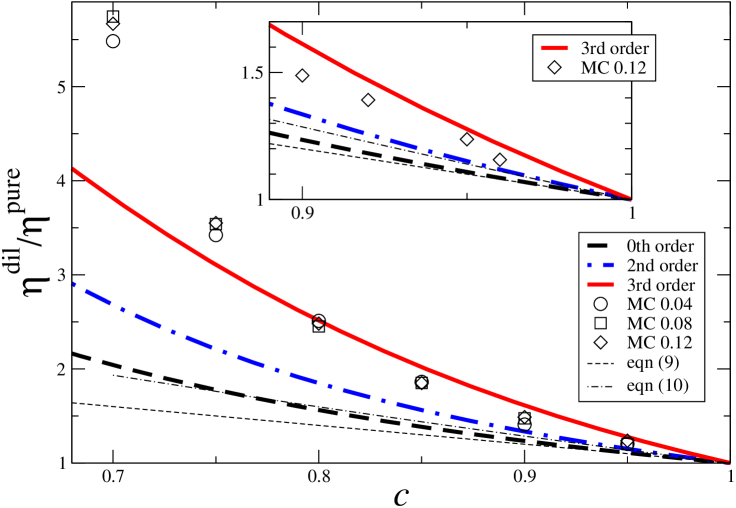
Figure 1: Comparison between the 1st (which in fact coincides with the 0th), 2nd and 3rd-order expansions and MC simulations at very low temperatures (the values of $(\beta J)^{-1}$ are indicated in the legend). Expressions (9) and (10) of the previous expansion are shown (thin lines) for comparison. Insert shows the vicinity of the pure system.

In order to check these expressions, simulations of 2D XY-spins are performed using Wolff’s cluster Monte Carlo algorithm [16]. The low-temperature phase being critical, local updates of single spins would suffer from the critical slowing down. Implemented in the case of the XY model, the Wolff algorithm first introduces bonds through the Ising variables defined by the sign of the projection of the spin variables along some random direction. Then clusters of sites are built by a bond percolation process (here the random graph model of the Fortuin-Kasteleyn representation). The percolation threshold for these bonds coincides with the Kosterlitz-Thouless point [17], which guarantees the efficiency of the Wolff cluster updating scheme [16] at $T_{\rm KT}$. In the low-temperature phase we are interested in, this algorithm could be less efficient, but nevertheless preferable to a local updating, since the correlation length is diverging. Using this procedure, we discard typically $10^{5}$ sweeps for thermalization, and the measurements are performed on typically $10^{5}$ production sweeps. Averages over disorder are performed using typically $10^{3}$ samples. There is no need of a better statistics. The boundary conditions are chosen periodic and the critical exponent $\eta(T)$ of the correlation function is measured indirectly through the finite-size scaling behaviour of the magnetization

$$M_{T}(L)\sim L^{-x_{\sigma}(T)},\quad x_{\sigma}(T)=\frac{1}{2}\eta(T),$$ (18)

where the last scaling relations holds in two dimensions.

In Figure 1, we compare the 0th to 3rd order expansions (remember that the 1rd order term vanishes) with the MC data. The agreement is quite good using the expansion parameter (11) which provides a clear improvement of the previous expansion given by expressions (9) and (10). Of course the question of the next order is not settled, but now we are on the way to counting higher orders or even summing the whole series. Another direction of future work would be to implement the same type of perturbation expansion within the Villain model [18] and to explore the deconfining transition of the diluted model.

References

• [1]
• [2] P.M. Chaikin, T.C. Lubensky, Principles of condensed matter physics, Cambridge University Press, Cambridge, 1995
• [3] D.R. Nelson, Defects and geometry in condensed matter physics, Cambridge University Press, Cambridge, 2002
• [4] V.L. Berezinskii, Sov. Phys. JETP 32 (1971) 493
• [5] J. M. Kosterlitz and D. J. Thouless, J. Phys. C: Solid State Phys. 6 (1973) 1181
• [6] J.M. Kosterlitz J. Phys. C: Solid State Phys. 7 (1974) 1046
• [7] N.D. Mermin and H. Wagner Phys. Rev. Lett. 22 (1966) 1133
• [8] P.C. Hohenberg, Phys. Rev. 158 (1967) 383
• [9] F. Wegner, Z. Phys. 206 (1967) 465
• [10] A.B. Harris, J. Phys. C 7 (1974) 1671
• [11] F. M. Paula, A. R. Pereira, and G. M. Wysin, Phys. Rev. B 72 (2005) 094425
• [12] G. M. Wysin, A. R. Pereira, I. A. Marques, S. A. Leonel, and P. Z. Coura, Phys. Rev. B 72 (2005) 094418
• [13] B. Berche, A. I. FariΓ±as-SΓ‘nchez, Yu.Β Holovatch, R.Β ParedesΒ V. Eur. Phys. J. B 36 (2003) 91
• [14] V.G. Vaks, A.I. Larkin, S.A. Pikin, Sov. Phys. ZhEPF 53 (1967) 281
• [15] G.A. Baker, Jr., P. Graves-Morris, PadΓ© Approximants, Addison-Wesley Publishing Co., Reading, Massachusetts, 1987
• [16] U. Wolff, Nucl. Phys. B 322 (1989) 759
• [17] I.Β Dukovski, J.Β Machta and L.V.Β Chayes, Phys. Rev. E 65 (2002) 026702
• [18] J. Villain, J. Physique 36 (1975) 581