Non-adiabatic Kohn-anomaly in a doped graphene monolayer

Abstract

We compute, from first-principles, the frequency of the E_2g, ${\bm{\Gamma}}$ phonon (Raman $G$ band) of graphene, as a function of the charge doping. Calculations are done using i) the adiabatic Born-Oppenheimer approximation and ii) time-dependent perturbation theory to explore dynamic effects beyond this approximation. The two approaches provide very different results. While, the adiabatic phonon frequency weakly depends on the doping, the dynamic one rapidly varies because of a Kohn anomaly. The adiabatic approximation is considered valid in most materials. Here, we show that doped graphene is a spectacular example where this approximation miserably fails.

Graphene is a 2-dimensional plane of carbon atoms arranged in a honeycomb lattice. The recent demonstration of a field-effect transistor (FET) based on a few-layers graphene sheet has boosted the interest in this system geim ; kim05 ; ferrari06 . In particular, by tuning the FET gate-voltage $V_{g}$ it is possible to dope graphene by adding an excess surface electron charge. The actual possibility of building a FET with just one graphene monolayer maximizes the excess charge corresponding to a single atom in the sheet. In a FET-based experiment, graphene can be doped up to $3~{}10^{13}$  cm^-2 electron concentration geim ; kim05 , corresponding, in a monolayer, to a 0.2% valence charge variation. The resulting chemical-bond modification could induce a variation of bond-lengths and phonon-frequencies of the same order, which would be measurable. This would realize the dream of tuning the chemistry, within an electronic device, by varying $V_{g}$.

The presence of Kohn anomalies (KAs) kohn59 ; piscanec04 in graphene could act as a magnifying glass, leading to a variation of the optical phonon-frequencies much larger than the 0.2% expected in conventional systems. On the other hand, the phonon-frequency change induced by FET-doping could provide a much more precise determination of the KA, with respect to other experimental settings. KAs manifest as a sudden change in the phonon dispersion for a wavevector ${\bf q}\sim 2{\bf k}_{F}$, where ${\bf k}_{F}$ is a Fermi-surface wavevector kohn59 . The KA can be determined by studying the phonon frequency as a function of ${\bf q}$ by, e.g., inelastic x-ray, or neutron scattering. These techniques have a finite resolution, in ${\bf q}$ and energy, which limits the precision on the measured KA dispersion. In graphene, $2{\bf k}_{F}$ is proportional to $V_{g}$. This suggests an alternative way to study the KA, that is to measure the phonon frequency at a fixed ${\bf q}$ and to vary $2{\bf k}_{F}$ by changing $V_{g}$. Within this approach, one could use Raman scattering, which has a much better energy and momentum resolution than x-ray and neutron scattering. This approach is feasible for graphene, which has a KA for the Raman-active E_2g ${\bm{\Gamma}}$-phonon piscanec04 (Raman $G$-band).

In this paper, we compute the variation of phonon frequency of the Raman $G$-band (E_2g mode at ${\bm{\Gamma}}$) in a graphene monolayer, as a function of the Fermi level. First, the calculations are done using a fully ab-initio approach within the customary adiabatic Born-Oppenheimer approximation. Then, time-dependent perturbation theory (TDPT) is used to go beyond.

Ab-initio calculations are done within density functional theory (DFT), using the functional of Ref. pbe , plane waves (30 Ry cutoff) and pseudopotentials vanderbilt . The Brillouin zone (BZ) integration is done on a uniform $64\times 64\times 1$ grid. An electronic smearing of 0.01 Ry with the Fermi-Dirac distribution is used methfessel . The two-dimensional graphene crystal is simulated using a super-cell geometry with an interlayer spacing of 7.5 Å  (if not otherwise stated). Phonon frequencies are calculated within the approach of Ref. dfpt , using the PWSCF code pwscf . The Fermi-energy shift is simulated by considering an excess electronic charge which is compensated by a uniformly charged back-ground.

The dependence of the Fermi energy $\epsilon_{F}$ on the surface electron- concentration $\sigma$ is determined by DFT (Fig 1). In graphene, the gap is zero only for the two equivalent K and K’ BZ-points and the electron energy $\epsilon$ can be approximated as $\epsilon_{\pi^{*}/\pi}({\rm\bf K}+{\bf k})=\pm\beta k$ for the $\pi^{*}$ and $\pi$ bands, where ${\bf k}$ is a small vector. Within this approximation, at $T$ = 0 K temperature

$$\sigma={\rm sign}(\epsilon_{F})\frac{\epsilon_{F}^{2}}{\pi\beta^{2}}={\rm sign}(\epsilon_{F})\frac{\epsilon_{F}^{2}}{{\rm eV}^{2}}~{}10.36~{}10^{13}{\rm cm}^{-2}$$ (1)

where $\beta=5.52$ eV$\cdot$Å from DFT, ${\rm sign}(x)$ is the sign of $x$ and $\epsilon_{F}=0$ at the $\pi$ bands crossing. We remark that, from Fig 1, the typical electron-concentration obtained in experiments geim ; kim05 corresponds to an important Fermi-level shift ($\sim$0.5 eV). For such shift, the linearized bands are still a good approximation (Fig. 1).

Figure 1: Graphene monolayer. Upper panel: $\epsilon_{F}$ as a function of the surface electron-concentration $\sigma$ from DFT calculations and from linearized bands (at $T=300$ K). Lower panel: in-plane lattice spacing $a$ as a function of $\sigma$. The fitting function is Eq. 2 and the dashed line is from Ref. pietronero81 .

The dependence of the graphene lattice-spacing $a$ on $\sigma$, $a(\sigma)$, is obtained by minimizing $F(\sigma,A)=[E(\sigma,A)-E(0,A_{0})]/A$ with respect to $A$, where $E(\sigma,A)$ is the energy of the graphene unit-cell, $A$ is unit-cell area and $A_{0}=5.29$ Å² is the equilibrium $A$ nota1 at zero $\sigma$. $E(\sigma,A)$ is computed by DFT letting the inter-layer spacing, $L$, tend to infinity in order to eliminate the spurious interaction between the background and the charged sheet nota2 . $\Delta a(\sigma)=[a(\sigma)-a(0)]/a(0)$ was determined in Ref. pietronero81 for intecalated graphite on the basis of a semi empirical model. Using the same functional dependence as in Ref. pietronero81 , our DFT calculations are fitted by

$$\Delta a(\sigma)=6.748\cdot 10^{-6}|\sigma|^{3/2}+1.64\cdot 10^{-4}\sigma,$$ (2)

where $\sigma$ is in units of 10¹³ cm^-2. With $\sigma=3~{}10^{13}$ cm^-2, the lattice spacing variation is $\sim 0.05\%$, which is, as expected, of the same order of the valence-charge variation.

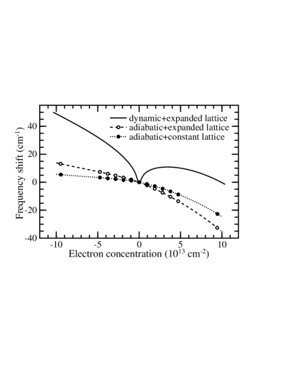
Figure 2: Frequency of the E_2g ${\bm{\Gamma}}$ phonon (Raman $G$ band) as a function of $\sigma$: shift with respect to the zero-doping frequency. Calculations are done using standard DFT (adiabatic) or TDPT (dynamic), keeping the lattice-spacing constant (constant lattice) or varying it according to Eq. 2 (expanded lattice). Points are DFT calculations. Dashed line is from Eq. 3. Experiments should be compared with the continuous line.

The frequency of the E_2g ${\bm{\Gamma}}$ phonon is computed by static perturbation theory of the DFT energy dfpt , i.e. from the linearized forces acting on the atoms due to the static displacement of the other atoms from their equilibrium positions. This approach is based on the adiabatic Born-Oppenheimer approximation, which is the standard textbook approach for phonon calculations and is always used, to our knowledge, in the ab-initio frequency calculations. The computed zero-doping phonon frequency is $\omega_{a}^{0}/(2\pi c)=1554$ cm^-1, where $c$ is the speed of light. The frequency variation $\Delta\omega$ with $\sigma$ is reported in Fig. 2. Calculations are done keeping the lattice-spacing constant at $a(0)$, or varying it according to Eq. 2. In this latter case, $\Delta\omega$ is fitted by

$$\frac{\Delta\omega}{2\pi c}=-2.13\sigma-0.0360\sigma^{2}-0.00329\sigma^{3}-0.226|\sigma|^{3/2},$$ (3)

where $\sigma$ is in 10¹³ cm^-2 and $\Delta\omega/(2\pi c)$ is in cm^-1 units. The lattice-parameter variation is important, since it nearly doubles the frequency shift. However, Fig. 2 does not show the sudden increase of the phonon frequency with $|\sigma|$, expected from the displacement of the KA wavevector with the doping. In particular, for $\sigma=$ 3 10¹³ cm^-2, the frequency variation is $\sim-0.5\%$, which excludes a magnification effect related to the KA.

It is important to understand whether the absence of the KA is an artifact of the adiabatic approximation, used so far. Thus, we consider that a phonon is not a static perturbation but a dynamic one, oscillating at the frequency $\omega$, which can be treated within time-dependent perturbation theory. Using such dynamic approach in the context of DFT allen , the dynamical matrix of a phonon with momentum ${\bf q}$, projected on the phonon normal-coordinate is

$${\cal D}^{\epsilon_{F}}_{\bf q}(\omega) = F^{\epsilon_{F}}_{\bf q}(\omega)+\int n({\bf r})\Delta^{2}V^{b}({\bf r})d^{3}r$$ (4)

$$-\int\Delta n^{*}_{\bf q}({\bf r})K({\bf r},{\bf r^{\prime}})\Delta n_{\bf q}({\bf r^{\prime}})d^{3}rd^{3}r^{\prime},$$

where $n({\bf r})$ is the charge density, $\Delta^{2}V^{b}$ is the second derivative of the bare (purely-ionic) potential with respect to the phonon displacement, $\Delta n$ is the derivative of $n$, $K({\bf r},{\bf r^{\prime}})=\delta^{2}E_{Hxc}[n]/(\delta n({\bf r})\delta n({\bf r^{\prime}}))$, $E_{Hxc}[n]$ is the Hartree and exchange-correlation functional, and

$$F^{\epsilon_{F}}_{{\bf q}}(\omega)=\frac{2}{N_{\bf k}}\sum_{{\bf k}nm}\frac{|D_{({\bf k+q})m,{\bf k}n}|^{2}[\tilde{f}_{({\bf k+q})m}-\tilde{f}_{{\bf k}n}]}{\epsilon_{({\bf k+q})m}-\epsilon_{{\bf k}n}+\hbar\omega+i\delta}.$$ (5)

Here a factor 2 accounts for spin degeneracy, the sum is performed on $N_{\bf k}$ wavevectors, $D_{({\bf k+q})m,{\bf k}n}=\langle({\bf k+q})m|\Delta V|{\bf k}n\rangle$ is the electron-phonon coupling (EPC), $\Delta V$ is the derivative of the Kohn-Sham potential, $|{\bf k}n\rangle$ is a Bloch eigenstate with wavevector ${\bf k}$, band index $n$ and energy $\epsilon_{{\bf k}n}$, $\tilde{f}_{{\bf k}n}=f_{T}(\epsilon_{{\bf k}n}-\epsilon_{F})$, where $f_{T}$ is the Fermi-Dirac distribution and $\delta$ is a small real number.

Imposing $\omega=0$ and $\delta=0$ in Eq. 4, one obtains the standard adiabatic approximation dfpt and the phonon frequency is $\omega^{\epsilon_{F}}_{a}=\sqrt{{\cal D}^{\epsilon_{F}}_{\bf q}(0)/M}$, where $M$ is the atomic mass. In the dynamic case, $\omega$ has to be determined self-consistently from $\omega=\sqrt{{\cal D}^{\epsilon_{F}}_{\bf q}(\omega)/M}$. However, considering dynamic and doping effects as perturbations, at the lowest order one can insert the adiabatic zero-doping phonon frequency $\omega_{a}^{0}$ in Eq 4 and obtain the real part of the dynamic frequency from $\omega^{\epsilon_{F}}_{d}=\Re\mathrm{e}\sqrt{{\cal D}^{\epsilon_{F}}_{\bf q}(\omega_{a}^{0})/M}$.

Let us consider the ${\bf q}\rightarrow{\bf 0}$ limit in Eq. 5. In the adiabatic case

$$F^{\epsilon_{F}}_{\bf 0}(0) = \frac{2}{N_{\bf k}}\sum_{{\bf k},n\neq m}\frac{|D_{{\bf k}m,{\bf k}n}|^{2}[\tilde{f}_{{\bf k}m}-\tilde{f}_{{\bf k}n}]}{\epsilon_{{\bf k}m}-\epsilon_{{\bf k}n}}$$ (6)

$$-\frac{2}{N_{\bf k}}\sum_{{\bf k},n}|D_{{\bf k}n,{\bf k}n}|^{2}\delta_{T}(\epsilon_{{\bf k}n}-\epsilon_{F}),$$

where $\delta_{T}(x)=-df_{T}(x)/(dx)$. In the dynamic case

$$F^{\epsilon_{F}}_{\bf 0}(\omega_{a}^{0}) = \frac{2}{N_{\bf k}}\sum_{{\bf k},n\neq m}\frac{|D_{{\bf k}m,{\bf k}n}|^{2}[\tilde{f}_{{\bf k}m}-\tilde{f}_{{\bf k}n}]}{\epsilon_{{\bf k}m}-\epsilon_{{\bf k}n}+\hbar\omega_{a}^{0}+i\delta}.$$ (7)

In Eq. 6 (adiabatic case), there are two contributions, the first from inter-band and the second from intra-band transitions (depending on $\delta_{T}$ and proportional to the density of states at $\epsilon_{F}$). On the contrary, in Eq. 7 (dynamic case) only inter-band transitions contribute.

The variation of $\omega^{\epsilon_{F}}$ with $\epsilon_{F}$ is

$$\Delta\omega=\omega^{\epsilon_{F}}-\omega^{0}\simeq\frac{{\cal D}^{\epsilon_{F}}-{\cal D}^{0}}{2M\omega^{0}_{a}},$$ (8)

where is assumed that $\Delta\omega\ll\omega^{0}_{a}$. The presence of a Kohn anomaly is associated to a singularity in the electron screening, which, within the present formalism, can occur if the denominator of Eq. 5 approaches zero, i.e. for electrons near the Fermi level. Let us call $\tilde{F}^{\epsilon_{f}}(\omega)$ the part of $F^{\epsilon_{F}}_{0}(\omega)$ obtained by restricting the k-sum on a circle of radius $\bar{k}$ centered on K, with $(\beta{\bar{k}}-|\epsilon_{F}|-\hbar\omega^{0}_{a})\gg k_{\rm B}T$. The anomalous $\Delta\omega$ is obtained by substituting ${\cal D}$ with $\tilde{F}$ nota04 in Eq. 8

$$\Delta\omega_{a} = \frac{\tilde{F}^{\epsilon_{F}}(0)-\tilde{F}^{0}(0)}{2M\omega^{0}_{a}}$$ (9)

$$\Delta\omega_{d} = \Re\mathrm{e}\left[\frac{\tilde{F}^{\epsilon_{F}}(\omega^{0}_{a})-\tilde{F}^{0}(\omega^{0}_{a})}{2M\omega^{0}_{a}}\right]$$ (10)

in the adiabatic ($\Delta\omega_{a}$) and dynamic ($\Delta\omega_{d}$) cases. An analytic expression for $\tilde{F}$ is obtained by i) linearizing the band dispersion; ii) writing the EPC as $|D_{({\bf K+k})n,({\bf K+k})m}|^{2}=\langle D^{2}_{\bm{\Gamma}}\rangle[1\pm\cos(2\theta)]$, where $\theta$ is the angle between the phonon-polarization and ${\bf k}$, the sign $\pm$ depends on the transition (see Eq. 6 and note 24 of Ref. piscanec04 ) and $\langle D^{2}_{\bm{\Gamma}}\rangle=45.6$ (eV)²/Å^-2 from DFT  lazzeri06 ; iii) substituting $1/N_{\bf k}\sum_{{\bf k}}$ with $2A_{0}/(2\pi)^{2}\int d^{2}k$ in Eqs. 6-7 , a factor 2 counts K and K’, and ${\bf k}$ is measured from K.

In the adiabatic case

$$\tilde{F}^{\epsilon_{F}}(0) = \alpha\int_{0}^{\bar{k}}kdk\left\{\frac{f_{T}(\beta k-\epsilon_{F})-f_{T}(-\beta k-\epsilon_{F})}{\beta k}\right.$$ (11)

$$-\left.\delta_{T}(\beta k-\epsilon_{F})-\delta_{T}(-\beta k-\epsilon_{F})\right\},$$

where $\alpha=2A_{0}\langle D^{2}_{\bm{\Gamma}}\rangle/\pi$. Substituting Eq. 11 into Eq. 9 one obtains $\Delta\omega_{a}$. At any $T$, $\Delta\omega_{a}=0$. This result is not trivial and comes from the exact cancellation of the inter-band ($\pi$ to $\pi^{*}$, first line of Eq. 11) and intra-band ($\pi$ to $\pi$ and $\pi^{*}$ to $\pi^{*}$, second line of Eq. 11). For example, at $T=0$, both contributions to $\hbar\Delta\omega_{a}$ are large and equal to $\alpha^{\prime}|\epsilon_{F}|$ and $-\alpha^{\prime}|\epsilon_{F}|$, respectively, where $\alpha^{\prime}=\hbar\alpha/(2M\omega^{0}_{a}\beta^{2})=4.43~{}10^{-3}$ and $\alpha^{\prime}/(2\pi\hbar c)=35.8$ cm${}^{-1}/(eV)$. Concluding, an adiabatic calculation of $\omega^{\epsilon_{F}}$ does not show any singular behavior in $\epsilon_{F}$ related to the Kohn anomaly, in agreement with the state-of-the-art adiabatic DFT calculations of Fig. 2.

In the dynamic case

$$\tilde{F}^{\epsilon_{F}}(\omega^{0}_{a})=\alpha\int_{-{\bar{k}}}^{\bar{k}}\frac{f_{T}(\beta k-\epsilon_{F})-f_{T}(-\beta k-\epsilon_{F})}{2\beta k+\hbar\omega^{0}_{a}+i\delta}|k|dk.$$ (12)

Substituting Eq. 12 into Eq. 10, for $T=0$,

$$\hbar\Delta\omega_{d}=\alpha^{\prime}|\epsilon_{F}|+\frac{\alpha^{\prime}\hbar\omega^{0}_{a}}{4}\ln\left(\left|\frac{|\epsilon_{F}|-\frac{\hbar\omega^{0}_{a}}{2}}{|\epsilon_{F}|+\frac{\hbar\omega^{0}_{a}}{2}}\right|\right).$$ (13)

In this case, the situation is very different since the large inter-band contribution is not canceled by an intra-band term. In particular, there are two logarithmic divergences for $\epsilon_{F}=\pm\hbar\omega^{0}_{a}/2$ and for $|\epsilon_{F}|\gg\hbar\omega^{0}_{a}/2$ the frequency increases as $\alpha^{\prime}|\epsilon_{F}|$.

$\Delta\omega_{d}$ computed in this way takes into account transitions between states close to the Fermi level. However, the frequency is also affected by the variation of the lattice-spacing, by the transitions involving a state far from $\epsilon_{F}$ and by the second and third terms in Eq. 4. All these contributions are accurately described by our adiabatic DFT calculations. Therefore, to compare with experiments, we add $\Delta\omega_{d}$ to the adiabatic DFT frequency shift of Eq. 3. The results are shown in Fig. 2 for $T=300~{}K$, and in Fig. 3 as a function of $T$ for a smaller $\sigma$ range. Even at room temperature, the non-adiabatic Kohn anomaly magnifies the effect of the doping and for a valence-charge variation of -0.2% (+0.2%), the frequency varies by +1.5% (+0.7%). $\Delta\omega$ is asymmetric with respect to $\epsilon_{F}$ and has a maximum for $\sigma\sim+3.5~{}10^{13}$ cm^-2. Since $\Delta\omega_{d}$ is an even function of $\epsilon_{F}$, this lack of electron-hole symmetry is entirely due to the adiabatic DFT contribution. The $\epsilon_{F}=\pm\hbar\omega^{0}_{a}/2$ logarithmic anomalies are visible at $T=4$ and$~{}70$ K. The presence of a logarithmic KA in this two-dimensional system is quite remarkable since such divergences are typical of one-dimensional systems. They are present in graphene because of its particular massless Dirac-like electron band dispersion.

Finally, the Raman $G$-band has a finite homogeneous linewidth due to the decay of the phonon into electron-hole pairs. Such EPC broadening can be obtained either from the imaginary part of the TDPT dynamical matrix (Eq. 12) or, equivalently, from the Fermi golden rule lazzeri06 :

$$\gamma=\frac{\pi}{2}\frac{\omega_{a}^{0}}{2\pi c}\alpha^{\prime}\left[f_{T}\left(-\frac{\hbar\omega_{a}^{0}}{2}-\epsilon_{F}\right)-f_{T}\left(\frac{\hbar\omega_{a}^{0}}{2}-\epsilon_{F}\right)\right]$$ (14)

where $\gamma$ is the full-width half-maximum (FWHM) in cm^-1. At $T=0$ and $\epsilon_{F}=0$, one recovers the result of Ref. lazzeri06 , $\gamma=11.0$ cm^-1. The phonon-phonon scattering contribution to the FWHM is smaller ($\sim$1 cm^-1 bonini ) and independent of $\epsilon_{F}$. The total homogeneous FWHM is reported in Fig. 3. The FWHM displays a strong doping dependence; it suddenly drops for $|\sigma|\sim 0.1~{}10^{13}$ cm^-2 ($|\epsilon_{F}|\sim 0.1$ eV). Indeed, because of the energy and momentum conservation, a ${\bm{\Gamma}}$ phonon decays into one electron (hole) with energy $\hbar\omega_{a}^{0}/2$ above (below) the level crossing. At $T=0K$ such process is compatible with the Pauli exclusion-principle only if $|\epsilon_{F}|<\hbar\omega_{a}^{0}/2$.

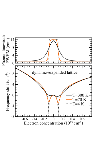
Figure 3: (Color online) Linewidth and dynamic frequency of the E_2g ${\bm{\Gamma}}$ mode (Raman $G$ band). See the caption of Fig. 1.

Concluding, a Kohn anomaly dictates the dependence of the highest optical-phonon on the wavevector ${\bf q}$, in undoped graphene  piscanec04 . Here, we studied the impact of such anomaly on the ${\bf q=0}$ phonon, as a function of the charge-doping $\sigma$. We computed, from first-principles, the phonon frequency and linewidth of the E_2g, ${\bm{\Gamma}}$ phonon (Raman $G$ band) in the $\sigma$-range reached by recent FET experiments. Calculations are done using i) the customary adiabatic Born-Oppenheimer approximation and ii) time-dependent perturbation theory to explore dynamic effects beyond this approximation. The two approaches provide very different results. The adiabatic phonon frequency displays a smooth dependence on $\sigma$ and it is not affected by the Kohn anomaly. On the contrary, when dynamic effects are included, the phonon frequency and lifetime display a strong dependence on $\sigma$, due to the Kohn anomaly. The variation of the Raman $G$-band with the doping in a graphene-FET has been recently measured by two groups kim07 ; ferrari07 . Both experiments are well described by our dynamic calculation but not by the more approximate adiabatic one. We remark that the adiabatic Born-Oppenheimer approximation is considered valid in most materials and is commonly used for phonon calculations. Here, we have shown that doped graphene is a spectacular example where this approximation miserably fails.

We aknowledge useful discussions with A.M. Saitta, A.C. Ferrari and S. Piscanec. Calculation were done at IDRIS (Orsay, France), project n^o 061202.

References

- (1) K.S. Novoselov et al. Science 306, 666 (2004); K.S. Novoselov et al. Nature 438, 197 (2005).
- (2) Y. Zhang, Y.W. Tan, H.L. Stormer, and P. Kim, Nature 438, 201 (2005).
- (3) A.C. Ferrari et al., Phys. Rev. Lett. 97, 187401 (2006).
- (4) W. Kohn Phys. Rev. Lett. 2, 393 (1959).
- (5) S. Piscanec, M. Lazzeri, F. Mauri, A.C. Ferrari, and J. Robertson, Phys. Rev. Lett. 93, 185503 (2004).
- (6) J.P. Perdew, K. Burke, and M. Ernzerhof Phys. Rev. Lett. 77, 3865 (1996).
- (7) D. Vanderbilt, Phys. Rev. B 41, 7892 (1990).
- (8) M. Methfessel and A.T. Paxton Phys. Rev. B 40, 3616 (1989).
- (9) S. Baroni, S. de Gironcoli, A. Dal Corso, and P. Giannozzi, Rev. Mod. Phys. 73, 515 (2001).
- (10) S. Baroni et al. http://www.pwscf.org.
- (11) Consider a graphene sample of unit-cells, which is in contact with an electrode of area . If , is obtained by minimizing the total energy of the sample . This is equivalent to minimizing .
- (12) By a simple electrostatic model, the dependence of the cell-energy on is . is computed for Å and the parameters , are fitted to obtain the limit .
- (13) L. Pietronero and S. Strässler Phys. Rev. Lett. 47, 593 (1981).
- (14) Eqs. 4.17a and 4.23 of P.B. Allen, in Dynamical Properties of Solids, Ed. by G. K. Horton and A.A. Maradudin, (North-Holland, Amsterdam, 1980), v. 3, p. 95-196.
- (15) The dependence of on and is neglected, because the functional of Eq. 4 is stationary with respect to . Notice that there are other, equivalent expressions for the dynamical matrix which are not stationary in , for which this approximation is not justified.
- (16) M. Lazzeri, S. Piscanec, F. Mauri, A.C. Ferrari, and J. Robertson, Phys. Rev. B 73, 155426 (2006).
- (17) N. Bonini, M. Lazzeri, F. Mauri, N. Marzari unpublished.
- (18) J. Yan, Y. Zhang, P. Kim, and A. Pinczuk (2006), unpublished. Results shown the 28 Sept. 2006 at the Graphene Conference, Max Planck Institut, Dresden.
- (19) S. Pisana, M. Lazzeri, C. Casiraghi, K.S. Novoselov, A.K. Geim, A.C. Ferrari, F. Mauri, cond-mat/0611714 (2006).