Universality class of 3D site-diluted and bond-diluted Ising systems

Abstract

We present a finite-size scaling analysis of high-statistics Monte Carlo simulations of the three-dimensional randomly site-diluted and bond-diluted Ising model. The critical behavior of these systems is affected by slowly-decaying scaling corrections which make the accurate determination of their universal asymptotic behavior quite hard, requiring an effective control of the scaling corrections. For this purpose we exploit improved Hamiltonians, for which the leading scaling corrections are suppressed for any thermodynamic quantity, and improved observables, for which the leading scaling corrections are suppressed for any model belonging to the same universality class.

The results of the finite-size scaling analysis provide strong numerical evidence that phase transitions in three-dimensional randomly site-diluted and bond-diluted Ising models belong to the same randomly dilute Ising universality class. We obtain accurate estimates of the critical exponents, $\nu=0.683(2)$, $\eta=0.036(1)$, $\alpha=-0.049(6)$, $\gamma=1.341(4)$, $\beta=0.354(1)$, $\delta=4.792(6)$, and of the leading and next-to-leading correction-to-scaling exponents, $\omega=0.33(3)$ and $\omega_{2}=0.82(8)$.

1 Introduction

The effect of quenched random disorder on the critical behavior of Ising systems has been much investigated experimentally and theoretically. Typical physical examples are randomly dilute uniaxial antiferromagnets, for instance, Fe_pZn_1-pF₂ and Mn_pZn_1-pF₂, obtained by mixing a uniaxial antiferromagnet with a nonmagnetic material. Experiments (see, e.g., Ref. [1] for a review) find that, for sufficiently low impurity concentration $1-p$, these systems undergo a second-order phase transition at $T_{c}(p)<T_{c}(p=1)$. The critical behavior appears approximately independent of the impurity concentration, but definitely different from the one of the pure system. These results support the existence of a random Ising universality class which differs from the one of pure Ising systems.

A simple lattice model for dilute Ising systems is provided by the three-dimensional randomly site-diluted Ising model (RSIM) with Hamiltonian

$${\cal H}_{s}=-J\,\sum_{<xy>}\rho_{x}\,\rho_{y}\;\sigma_{x}\sigma_{y},$$ (1)

where the sum is extended over all nearest-neighbor sites of a simple cubic lattice, $\sigma_{x}$ are Ising spin variables, and $\rho_{x}$ are uncorrelated quenched random variables, which are equal to one with probability $p$ (the spin concentration) and zero with probability $1-p$ (the impurity concentration). Another related lattice model is the randomly bond-diluted Ising model (RBIM) with Hamiltonian

$${\cal H}_{b}=-J\,\sum_{<xy>}j_{xy}\;\sigma_{x}\sigma_{y},$$ (2)

where the bond variables $j_{xy}$ are uncorrelated quenched random variables, which are equal to one with probability $p$ and zero with probability $1-p$. Note that the RSIM can be seen as a RBIM with bond variables $\hat{\hbox{\em\j}}_{xy}=\rho_{x}\rho_{y}$. But in this case the bond variables are correlated. For example, the connected average of the bond variables along a plaquette does not vanish as in the case of uncorrelated bond variables: indeed (note that $\overline{\hat{\hbox{\em\j}}_{xy}}=p^{2}$)

$$\overline{\prod_{\square}(\hat{\hbox{\em\j}}_{xy}-\overline{\hat{\hbox{\em\j}}_{xy}})}=p^{4}-4p^{6}+4p^{7}-p^{8}.$$ (3)

Above the percolation threshold of the spins, these models undergo a phase transition between a disordered and a ferromagnetic phase. Its nature has been the object of many theoretical studies, see, e.g., Refs. [4, 5, 6, 7, 8] for reviews. A natural scenario is that the critical behavior of the RSIM and the RBIM, at any value of $p$ above the spin percolation threshold, belongs to the same universality class, which we will call randomly dilute Ising (RDIs) universality class.

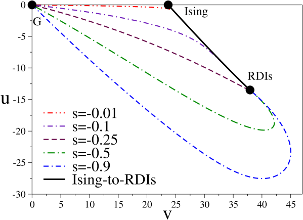
Figure 1: RG trajectories in the renormalized coupling $(u,v)$ plane starting from the Gaussian FP, for several values of the ratio $s\equiv u_{0}/v_{0}$ (from Ref. [9]). We also report the RG trajectory connecting the Ising FP with the RDIs FP, relevant for the Ising-to-RDIs crossover.

The RDIs universality class can be investigated by field-theoretical (FT) methods, starting from the Landau-Ginzburg-Wilson $\phi^{4}$ Hamiltonian

$$H_{\phi^{4}}=\int d^{d}x\Bigl{\{}{1\over 2}\sum_{i=1}^{N}\left[(\partial_{\mu}\phi_{i})^{2}+r\phi_{i}^{2}\right]+{1\over 4!}\sum_{i,j=1}^{N}\left(u_{0}+v_{0}\delta_{ij}\right)\phi^{2}_{i}\phi^{2}_{j}\Bigr{\}},$$ (4)

where $\phi_{i}$ is an $N$-component field. By using the standard replica trick, it can be shown that, for $u_{0}<0$ and in the limit $N\to 0$, this model corresponds to a system with quenched disorder effectively coupled to the energy density. Fig. 1 shows the renormalization-group (RG) flow [9] in the $u,v$ plane, where $u,v$ are the renormalized couplings associated with the Hamiltonian parameters $u_{0}$ and $v_{0}$. The RG flow has a stable fixed point (FP) in the region $u<0$, which attracts systems with $-1\mathrel{\hbox to0.0pt{\lower 3.0pt\hbox{$\mathchar 536\relax$}\hss}\raise 2.0pt\hbox{$\mathchar 316\relax$}}u_{0}/v_{0}<0$. The standard Ising FP at $u=0$ is unstable, with a crossover exponent [4] $\phi=\alpha_{\rm Is}$, where [10] $\alpha_{\rm Is}=0.1096(5)$ is the specific-heat exponent of the Ising universality class. The stable RDIs FP determines the critical behavior at the phase transition between the disordered and the ferromagnetic phase that occurs in RDIs systems. Therefore, it is expected to determine the critical behavior of the RSIM and of the RBIM above the spin percolation threshold. The critical exponents at the RDIs FP have been computed perturbatively to six loops in the three-dimensional massive zero-momentum scheme [11, 12]. Even though the perturbative series are not Borel summable [13, 14, 15], appropriate resummations provide quite accurate results [11]: $\nu=0.678(10)$, $\alpha=-0.034(30)$, $\eta=0.030(3)$, $\gamma=1.330(17)$, $\beta=0.349(5)$. Moreover, the leading scaling corrections are characterized by a small exponent $\omega=0.25(10)$, which is much smaller than that occurring in pure Ising systems, $\omega\approx 0.8$ [16, 6]. Experiments find [1] $\nu=0.69(1)$, $\alpha=-0.10(2)$, and $\beta=0.350(9)$, which are in reasonable agreement with the FT estimates (there is only a small discrepancy for $\alpha$). We also mention that approximate expressions for the RDIs critical equation of state have been reported in Ref. [17].

Monte Carlo (MC) simulations of the RSIM and the RBIM have long been inconclusive in settling the question of the critical behavior of these models. While the measured critical exponents were definitely different from the Ising ones, results apparently depended on the spin concentration, in disagreement with RG theory. The question was clarified in Ref. [18], where the apparent violations of universality were explained by the presence of large concentration-dependent scaling corrections, which decay very slowly because of the small value of the exponent $\omega$, $\omega=0.37(6)$. Only if they are properly taken into account, the numerical estimates of the critical exponents of the RSIM become dilution-independent as expected. Ref. [18] reported the estimates $\nu=0.6837(53)$ and $\eta=0.0374(45)$, which are in agreement with the FT results. These results were later confirmed by MC simulations [19] of the RSIM at $p=0.8$, which is the value of $p$ where the leading scaling corrections appear suppressed [18, 20]. A FSS analysis of the data up to lattice size $L=256$ gave $\nu=0.683(3)$ and $\eta=0.035(2)$. On the other hand, results for the RBIM have been less satisfactory. Recent works, based on FSS analyses [21] of MC data up to $L=96$ and high-temperature expansions [22], have apparently found asymptotic power-law behaviors that are quite dependent on the spin concentration. Such results may again be explained by the presence of sizeable and spin-concentration dependent scaling corrections.

The RSIM and the RBIM, and in general systems which are supposed to belong to the RDIs universality class, are examples of models in which the presence of slowly-decaying scaling corrections makes the determination of the asymptotic critical behavior quite difficult. In these cases, the universal critical behavior can be reliably determined only if scaling corrections are kept under control in the numerical analyses. For example, the Wegner expansion of the magnetic susceptibility $\chi$ is generally given by [23]

$$\chi = Ct^{-\gamma}\left(1+a_{0,1}t+a_{0,2}t^{2}+\ldots+a_{1,1}t^{\Delta}+a_{1,2}t^{2\Delta}+\ldots\right.$$ (5)

$$\left.\qquad+b_{1,1}t^{1+\Delta}+b_{1,2}t^{1+2\Delta}+\ldots+a_{2,1}t^{\Delta_{2}}+\ldots\right),$$

where $t\equiv 1-\beta/\beta_{c}$ is the reduced temperature. We have neglected additional terms due to other irrelevant operators and terms due to the analytic background present in the free energy [24, 25, 26]. In the case of the three-dimensional RDIs universality class we have [18, 11] $\Delta=\omega\nu\approx 0.2$, which is very small, and [19] $\Delta_{2}=\omega_{2}\nu\approx 0.5$. Analogously, the finite-size scaling (FSS) behavior at criticality is given by [25, 27]

$$\chi=cL^{2-\eta}\left(1+a_{1,1}L^{-\omega}+a_{1,2}L^{-2\omega}+\ldots+a_{2,1}L^{-\omega_{2}}+\ldots\right),$$ (6)

where $\omega\approx 0.3$ and $\omega_{2}\approx 0.8$ for the RDIs universality class.

The main purposes of this paper are the following:

• We wish to improve the numerical estimates of the critical exponents associated with the asymptotic behavior and with the leading scaling corrections.

• We wish to provide robust evidence that the critical behaviors of the RSIM and of the RBIM belong to the same RDIs universality class, independently of the impurity concentration.

For these purposes, we perform a high-statistics MC simulation of the RSIM for $p=0.8$ and $p=0.65$, and of the RBIM for $p=0.7$ and $p=0.55$, for lattice sizes up to $L=192$. The critical behavior is obtained by a careful FSS analysis, in which a RG invariant quantity (we shall use $R_{\xi}\equiv\xi/L$) is kept fixed. This method has significant advantages [28, 29, 27] with respect to more standard approaches, and, in particular, it does not require a precise estimate of $\beta_{c}$. Our main results can be summarized as follows.

• We obtain accurate estimates of the critical exponents: $\nu=0.683(2)$ and $\eta=0.036(1)$. Then, using the scaling and hyperscaling relations $\alpha=2-3\nu$, $\gamma=(2-\eta)\nu$, $\beta=\nu(1+\eta)/2$ and $\delta=(5-\eta)/(1+\eta)$, we obtain $\alpha=-0.049(6)$, $\gamma=1.341(4)$, $\beta=0.354(1)$, and $\delta=4.792(6)$.

• We obtain accurate estimates of the exponents associated with the leading scaling corrections: $\omega=0.33(3)$ and $\omega_{2}=0.82(8)$. Correspondingly, we have $\Delta=\omega\nu=0.22(2)$ and $\Delta_{2}=\omega_{2}\nu=0.56(5)$.

• For both the RSIM and the RBIM we estimate the value $p^{*}$ at which the leading scaling corrections associated with the exponent $\omega$ vanish for all quantities. For the RSIM, we find $p^{*}=0.800(5)$. This result significantly strengthens the evidence that the RSIM with $p=0.8$ is improved, as already suggested by earlier calculations [18, 19]. For the RBIM, we find $p^{*}=0.54(2)$.

• We provide strong evidence that the transitions in the RSIM and in the RBIM belong to the same universality class. For this purpose, the knowledge of the leading and next-to-leading scaling correction exponents is essential. We also make use of improved observables characterized by the (approximate) absence of the leading scaling correction for any system belonging to the RDIs universality class.

The paper is organized as follows. In Sec. 2 we report the definitions of the quantities which are considered in the paper. In Sec. 3 we summarize some basic FSS results which are needed for the analysis of the MC data. In Sec. 4 we give some details of the MC simulations. Sec. 5 describes the FSS analyses of the MC data of the RSIM at $p=0.8$ and $p=0.65$ at fixed $R_{\xi}$, which lead to the best estimates of the critical exponents. FSS analyses at fixed $\beta$ of the RSIM at $p=0.8$ are presented in Sec. 6. Finally, in Sec. 7 we analyze the data for the RBIM at $p=0.55$ and $p=0.7$, and show that the RBIM belongs to the same universality class as the RSIM. In A we determine the next-to-leading correction-to-scaling exponent $\omega_{2}$ by a reanalysis of the FT six-loop perturbative expansions reported in Ref. [30]. In B we discuss the problem of the bias in MC calculations of disorder averages of combinations of thermal averages.

2 Notations

We consider Hamiltonians (1) and (2) with $J=1$ on a finite simple-cubic lattice $L^{3}$ with periodic boundary conditions. In the case of the RSIM, given a quantity ${\cal O}$ depending on the spins $\{\sigma\}$ and on the random variables $\{\rho\}$, we define the thermal average at fixed distribution $\{\rho\}$ as

$$\langle{\cal O}\rangle(\beta,\{\rho\})\equiv{1\over Z(\{\rho\})}\sum_{\{\sigma\}}{\cal O}e^{-\beta{\cal H}[\sigma,\rho]},$$ (7)

where $Z(\{\rho\})$ is the sample partition function. Then, we average over the random dilution considering

$$\overline{\langle{\cal O}\rangle}(\beta)=\int[d\rho]\langle{\cal O}\rangle(\beta,\{\rho\}),$$ (8)

where

$$[d\rho]=\prod_{x}[p\delta(\rho_{x}-1)+(1-p)\delta(\rho_{x})].$$ (9)

Analogous formulas can be written for the RBIM, taking

$$[dj]=\prod_{<xy>}[p\delta(j_{xy}-1)+(1-p)\delta(j_{xy})].$$ (10)

We define the two-point correlation function

$$G(x)\equiv\overline{\langle\rho_{0}\sigma_{0}\,\rho_{x}\sigma_{x}\rangle}\qquad \hbox{(RSIM)},$$ (11)

$$G(x)\equiv\overline{\langle\sigma_{0}\,\sigma_{x}\rangle}\qquad \hbox{(RBIM)},$$

the corresponding susceptibility $\chi$,

$$\chi\equiv\sum_{x}G(x),$$ (12)

and the correlation length $\xi$,

$$\xi^{2}\equiv{\widetilde{G}(0)-\widetilde{G}(q_{\rm min})\over\hat{q}_{\rm min}^{2}\hat{G}(q_{\rm min})},$$ (13)

where $q_{\rm min}\equiv(2\pi/L,0,0)$, $\hat{q}\equiv 2\sin q/2$, and $\widetilde{G}(q)$ is the Fourier transform of $G(x)$.

We also consider quantities that are invariant under RG transformations in the critical limit. We call them phenomenological couplings and generically refer to them by using the symbol $R$. Beside the ratio

$$R_{\xi}=\xi/L,$$ (14)

we consider the quartic cumulants $U_{4}$ and $U_{22}$ defined by

$$U_{4}\equiv{\overline{\mu_{4}}\over\overline{\mu_{2}}^{2}},\qquad U_{22}\equiv{\overline{\mu_{2}^{2}}-\overline{\mu_{2}}^{2}\over\overline{\mu_{2}}^{2}},$$ (15)

where

$$\mu_{k}\equiv\langle\;(\sum_{x}\rho_{x}\sigma_{x}\;)^{k}\rangle\quad \quad{\rm(RSIM)},$$

$$\mu_{k}\equiv\langle\;(\sum_{x}\sigma_{x}\;)^{k}\rangle\quad \quad{\rm(RBIM)}.$$

We also define their difference

$$U_{d}\equiv U_{4}-U_{22}.$$ (17)

Finally, we consider the derivative of the phenomenological couplings $R$ with respect to the inverse temperature, i.e.,

$$R^{\prime}\equiv{\partial R\over\partial\beta},$$ (18)

which allows one to determine the critical exponent $\nu$.

3 Finite-size scaling

3.1 General results

In this section we summarize some basic results concerning FSS, which will be used in the FSS analysis. We consider a generic RDIs model in the presence of a constant magnetic field $H$ and in a finite volume of linear size $L$, and the disorder-averaged free-energy density

$${\cal F}(\beta,H,L)={1\over L^{d}}\overline{\ln Z(\beta,H,L)},$$ (19)

where $d$ is the space dimension ($d=3$ in our specific case). In analogy with what is found in systems without disorder (see, e.g., Refs. [25, 31]), we expect the free energy to be the sum of a regular part ${\cal F}_{\rm reg}(\beta,H,L)$ and of a singular part ${\cal F}_{\rm sing}(\beta,H,L)$. The regular part is expected to depend on $L$ only through exponentially small terms, while the singular part encodes the critical behavior. The scaling behavior of the latter is expected to be:

$${\cal F}_{\rm sing}(u_{t},u_{h},\{u_{i}\},L)=L^{-d}{\cal F}_{\rm sing}(L^{y_{t}}u_{t},L^{y_{h}}u_{h},\{L^{y_{i}}u_{i}\}),$$ (20)

where $u_{t}\equiv u_{1}$, $u_{h}\equiv u_{2}$, $\{u_{i}\}$ with $i\geq 3$ are the scaling fields associated respectively with the reduced temperature $t$ ($u_{t}\sim t$), the magnetic field $H$ ($u_{h}\sim H$), and the other irrelevant perturbations with $y_{i}<0$. They are analytic functions of the Hamiltonian parameters—in particular, of $t$ and $H$—and are expected not to depend on the linear size $L$ [25]. Since $u_{t}$ and $u_{h}$ are assumed to be the only relevant scaling fields, $y_{i}<0$ for $i\geq 3$. Thus, in the infinite-volume limit and for any $t$, the arguments $L^{y_{i}}u_{i}$ go to zero. One may thus expand ${\cal F}_{\rm sing}$ with respect to $L^{y_{i}}u_{i}$ obtaining all scaling corrections. The RG dimensions of the relevant scaling fields $u_{t}$ and $u_{h}$ are related to the standard exponents $\nu$ and $\eta$ by $y_{t}=1/\nu$ and $y_{h}=(d+2-\eta)/2$. The correction-to-scaling exponents $\omega$ and $\omega_{2}$ introduced in Sec. 1 are related to the RG dimensions of the two leading irrelevant scaling fields: $\omega=-y_{3}$ and $\omega_{2}=-y_{4}$.

The scaling behavior of zero-momentum thermodynamic quantities can be obtained by performing appropriate derivatives of Eq. (20) with respect to $t$ and $H$. For instance, for the susceptibility at $H=0$ we obtain

$$\chi(\beta,L)=k_{\chi}L^{2-\eta}\left[\chi_{0}(u_{t}L^{y_{t}})+\sum_{i\geq 3}^{\infty}\sum_{k}\chi_{i,k}(u_{t}L^{y_{t}})\,u_{i}^{k}L^{ky_{i}}\right]+\chi_{\rm reg}(\beta),$$ (21)

where we have neglected terms scaling as $L^{y_{t}-2y_{h}}$, $L^{y_{i}-y_{h}}$, and $L^{y_{i}+y_{j}-2y_{h}}$, which arise from the $H$ dependence of $u_{t}$ and $u_{i}$ (see, e.g., Refs. [24, 32] for a discussion in the infinite-volume limit). The functions $\chi_{0}(z)$ and $\chi_{i,k}(z)$ are smooth, finite for $z\to 0$, and universal once one chooses a specific normalization condition (which must be independent of the Hamiltonian parameters) for the scaling fields and for the susceptibility (which amounts to properly choosing the model-dependent constant $k_{\chi}$). The function $\chi_{\rm reg}(\beta)$ represents the contribution of the regular part of the free-energy density and is $L$ independent (apart from exponentially small terms). For $t\to 0$ we have $u_{t}(t=0)=0$, while, generically, we expect $u_{i}(t=0)\not=0$. Expanding Eq. (21) for $L\to\infty$, one obtains Eq. (6).

Analogous formulae hold for the $2n$-point susceptibilities. They allow us to derive the scaling behavior of the quartic cumulant $R=U_{4}$. We obtain in the FSS limit

$$R(\beta,L)=r_{0}(u_{t}L^{y_{t}})+\sum_{i\geq 3}^{\infty}\sum_{k}r_{i,k}(u_{t}L^{y_{t}})\,u_{i}^{k}L^{ky_{i}}+r_{\rm reg}(\beta),$$ (22)

where again several irrelevant terms have been neglected. As before, the functions $r_{0}(z)$ and $r_{i,k}(z)$ are smooth, finite for $z\to 0$, and universal. The function $r_{\rm reg}(\beta)$ is due to the regular part of the free energy and gives rise to scaling corrections of order $L^{\eta-2}$. For $t\to 0$, writing $u_{t}=c_{t}t+O(t^{2})$, we can further expand Eq. (22), obtaining

$$R(\beta,L)=R^{*}+{r}_{0}^{\prime}(0)c_{t}\,tL^{y_{t}}+r_{3,0}(0)u_{3}(t=0)\,L^{y_{3}}+r_{3,1}(0)u_{3}(t=0)^{2}\,L^{2y_{3}}$$

$$+r_{4,0}(0)u_{4}(t=0)\,L^{y_{4}}+O(t^{2}L^{2y_{t}},L^{3y_{3}},tL^{y_{t}+y_{3}},L^{2y_{4}},L^{y_{5}}),$$ (23)

where $R^{*}\equiv r_{0}(0)$ and we have not written explicitly the corrections due to $r_{\rm reg}(\beta)$. Note that no analytic $1/L$ corrections are expected [25, 27].

The scaling behavior of $U_{22}$ can be derived analogously. In this case, one should start from the two-replica free-energy density (see, e.g., Ref. [17], App. B)

$${\cal F}_{2}(\beta,H_{1},H_{2},L)={1\over L^{d}}\overline{\ln Z(\beta,H_{1},L)\ln Z(\beta,H_{2},L)}$$ (24)

and assume, as before, that ${\cal F}_{2}(\beta,H_{1},H_{2},L)$ is the sum of a regular part and of a singular part. The latter should scale as

$${\cal F}_{2,\rm sing}(u_{t},u_{h_{1}},u_{h_{2}},\{u_{i}\},L)=L^{-d}{\cal F}_{\rm sing}(L^{y_{t}}u_{t},L^{y_{h}}u_{h_{1}},L^{y_{h}}u_{h_{2}},\{L^{y_{i}}u_{i}\}),$$ (25)

where we have now two magnetic scaling fields such that $u_{h_{1}}\sim H_{1}$ and $u_{h_{2}}\sim H_{2}$. Taking the appropriate derivatives, one can verify that Eq. (22) holds for $U_{22}$ too.

The discussion we have presented applies only to zero-momentum quantities. In order to derive the scaling behavior of the correlation length, we should also consider quantities that are defined in terms of the field variables at nonzero momentum. They can be derived from a free-energy density associated with a model in which the magnetic field is site dependent. The general analysis by Wegner [23] indicates that Eq. (25) should still hold (at least in systems without disorder; we assume here that the same holds for quenched averages): the presence of a site-dependent $H$ only modifies the scaling fields that become functionals of $H$. For these reasons, we conjecture that also $\xi$ has an expansion similar to (22): in particular, we expect corrections proportional to $u_{3}^{k}L^{-k\omega}$ and $u_{4}^{k}L^{-k\omega_{2}}$. The momentum dependence of the scaling fields will give rise to additional terms, the leading one being proportional to $L^{-2}$ (for a discussion in the two-dimensional Ising model, see Ref. [33], p. 8161). Additional $1/L^{2}$ corrections arise from our particular definition of $\xi$ [34]. The analyses we shall report below confirm this conjecture.

The scaling fields $u_{i}$ depend on the model. Thus, if one considers families of models that depend on an irrelevant parameter, by a proper tuning one can find Hamiltonians for which $u_{3}(t=0)=0$. In this case, in the FSS limit $t\to 0$, $L\to\infty$ at fixed $tL^{y_{t}}$, all corrections proportional to $L^{ky_{3}}=L^{-k\omega}$ vanish. Note that, since the scaling field depends only on the model, such a cancellation occurs for any quantity one considers. In all cases the leading correction-to-scaling term behaves as $L^{-\omega_{2}}$. Models such that $u_{3}(t=0)=0$ will be called improved models. Since the leading scaling correction vanishes, one should observe a faster approach to the scaling limit.

In this paper we shall also consider improved observables. An improved phenomenological coupling is such that $r_{3,0}(0)=0$. As a consequence, in the FSS limit at fixed $u_{t}L^{y_{t}}=0$ it does not show leading scaling corrections proportional to $L^{-\omega}$. Note that this cancellation is only observed on the line in the $(t,L)$ plane such that $tL^{y_{t}}=0$, but not in the generic FSS limit. As a consequence, if $R$ is improved, its derivative $R^{\prime}$ is not. Note also that, while in improved models all corrections proportional to $L^{-k\omega}$ vanish, here only the leading one vanishes: corrections proportional to $L^{-2\omega}$ are still present. Improved observables satisfy a very important property. Since the function $r_{3,0}(z)$ is universal, the cancellation occurs in any model.

The thermal RG exponent $y_{t}=1/\nu$ is usually computed from the FSS of the derivative $R^{\prime}$ of a phenomenological coupling $R$ with respect to $\beta$ at $\beta_{c}$. Using Eq. (22) one obtains

$$\left.R^{\prime}\right|_{\beta_{c}}=s_{0}L^{y_{t}}\left[1+a_{3}u_{3}(t=0)L^{y_{3}}+a_{4}u_{4}(t=0)L^{y_{4}}+b_{3}{du_{3}\over dt}(t=0)\,L^{y_{3}-y_{t}}+\ldots\right],$$ (26)

where $s_{0}$, $a_{3}$, $a_{4}$ are constants. The leading correction scales as $L^{y_{3}}=L^{-\omega}$. In improved models, in which $u_{3}(t=0)=0$, the leading correction is of order $L^{y_{4}}=L^{-\omega_{2}}$. Note that corrections proportional to $L^{y_{3}-y_{t}}=L^{-\omega-1/\nu}$ are still present even if the model is improved.

3.2 Finite-size scaling at a fixed phenomenological coupling

Instead of computing the various quantities at fixed Hamiltonian parameters, one may study FSS keeping a phenomenological coupling $R$ fixed at a given value $R_{f}$ [28]. This means that, for each $L$, one considers $\beta_{f}(L)$ such that

$$R(\beta=\beta_{f}(L),L)=R_{f}.$$ (27)

All interesting thermodynamic quantities are then computed at $\beta=\beta_{f}(L)$. The pseudocritical temperature $\beta_{f}(L)$ converges to $\beta_{c}$ as $L\to\infty$. The value $R_{f}$ can be specified at will, as long as $R_{f}$ is taken between the high- and low-temperature fixed-point values of $R$. The choice $R_{f}=R^{*}$ (where $R^{*}$ is the critical-point value) improves the convergence of $\beta_{f}$ to $\beta_{c}$ for $L\to\infty$; indeed [28, 35] $\beta_{f}-\beta_{c}=O(L^{-1/\nu})$ for generic values of $R_{f}$, while $\beta_{f}-\beta_{c}=O(L^{-1/\nu-\omega})$ for $R_{f}=R^{*}$. This method has several advantages. First, no precise knowledge of $\beta_{c}$ is needed. Secondly, for some observables, the statistical error at fixed $R_{f}$ is smaller than that at fixed $\beta=\beta_{c}$.

If $\beta_{f}$ is determined as in Eq. (27), one may consider the value of other phenomenological couplings $R_{\alpha}$ at $\beta_{f}$, defining

$$\bar{R}_{\alpha}(L)\equiv R_{\alpha}[\beta_{f}(L),L].$$ (28)

The large-$L$ limit of $\bar{R}_{\alpha}$ is universal but depends on $R_{f}$ (it differs from the critical value $R_{\alpha}^{*}$, unless $R_{f}=R^{*}$). Indeed, neglecting scaling corrections in Eq. (22), we have $R_{\alpha}=r_{\alpha;0}(u_{t}L^{y_{t}})$ and $R=r_{0}(u_{t}L^{y_{t}})$, where $r_{\alpha;0}(z)$ and $r_{0}(z)$ are universal functions. Fixing $R=R_{f}$ corresponds to fixing a particular trajectory in the $t,L$ plane given by $u_{t}L^{y_{t}}=z_{f}$, where $z_{f}$ is the solution of the equation $R_{f}=r_{0}(z_{f})$. Along this trajectory $R_{\alpha}=\bar{R}_{\alpha}=r_{\alpha;0}(z_{f})$, which shows the universality of $\bar{R}_{\alpha}$.

We can define improved observables also when considering FSS at fixed $R_{f}$. Such observables show a faster convergence since the corrections to the scaling limit scale as $L^{-\omega_{2}}$ and $L^{-2\omega}$. Moreover, at variance with the case discussed in Sec. 3.1 where it was practical to define an improved observable only on the line $tL^{y_{t}}=0$, here one can choose any value for $R_{f}$. If one determines an improved observable in a given model for a chosen value $R_{f}$, this observable is improved in any other model at the same value $R_{f}$.

4 Monte Carlo simulations

We performed MC simulations of the RSIM at $p=0.8$ and $p=0.65$ and of the RBIM at $p=0.55$ and $p=0.7$ close to the critical temperature on cubic lattices of size $L^{3}$, with $L=8$, $12$, $16$, $24$, $32$, $48$, $64$, $96$, $128$. For the RSIM at $p=0.8$ we also performed simulations with $L=192$. For each lattice size, we collected $N_{s}$ disorder samples, $N_{s}$ varying between $10^{4}$ and $6.4\times 10^{5}$. In Tables 1, 2, 3, 4, and 5 we report some details of the MC simulations and the results at fixed $R_{\xi}\equiv\xi/L=0.5943$.

In the simulations we used a combination of Metropolis, Swendsen-Wang (SW) cluster [36], and Wolff single-cluster [37] updates, to achieve an effective thermalization of short- and long-range modes. For each disorder sample, we started from a random spin configuration, then we typically performed 300 thermalization steps, each step consisting in 1 SW update, 1 Metropolis update, and $L$ single-cluster updates. Then, we typically performed 400 measures for lattice sizes $L\leq 64$ and 600 measures for larger lattices. Between two measurements we usually performed 1 SW update and $2L$ single-cluster Wolff updates. We did several tests of thermalization, performing some runs with a larger number of thermalization steps; to test the independence of the results on $N_{m}$, we also did few runs with a larger number of measures per disorder configuration.

In the determination of the averages over disorder one should take care of the bias that occurs because of the finite number of measures at fixed disorder [38]. A bias correction should be introduced whenever one considers the disorder average of combinations of thermal averages and, in particular, whenever a reweighting of the data is performed. Details are reported in B. Errors are computed from the sample-to-sample fluctuations and are determined by using the jackknife method.

The MC simulations that we present here took approximately 10 CPU years of a workstation equipped with an AMD Opteron Processor 246 (2 GHz clock frequency).

Table 1: Run parameters and estimates of $\beta_{f}$ and $\chi$ at fixed $R_{\xi}=0.5943$ for the RSIM at $p=0.8$. $N_{s}$ is the number of disorder samples divided by $1000$.

$L$	$N_{s}$	$\beta_{\rm run}$	$\beta_{f}$	$\chi$
8	200	0.285744	0.286020(24)	63.391(9)
12	200	0.285744	0.285851(14)	141.581(19)
16	200	0.285744	0.285800(6)	249.910(25)
24	100	0.285744	0.285765(6)	555.67(7)
32	100	0.285744	0.285751(4)	979.36(13)
	100	0.285761	0.285753(4)	979.27(12)
48	60	0.285744	0.2857515(24)	2173.7(3)
	106	0.285748	0.2857459(18)	2173.8(3)
	60	0.285751	0.285743(3)	2174.0(3)
64	60	0.285742	0.2857478(18)	3827.1(6)
	63	0.285744	0.2857443(17)	3827.4(6)
96	30	0.285744	0.2857441(13)	8491.6(1.9)
128	20	0.285743	0.2857428(9)	14950(4)
	20	0.285744	0.2857438(10)	14945(4)
192	10	0.285743	0.2857430(7)	33150(12)
	10	0.285744	0.2857435(8)	33141(13)

Table 2: MC results for the phenomenological couplings at fixed $R_{\xi}=0.5943$ for the RSIM at $p=0.8$.

$L$	$\beta_{\rm run}$	$\bar{U}_{22}$	$\bar{U}_{4}$	$\bar{U}_{d}$	$\bar{U}_{\rm im}$	$\bar{R^{\prime}}_{\xi}$	$-\bar{U^{\prime}}_{4}$
8	0.285744	0.1504(6)	1.6066(5)	1.45624(19)	1.8021(14)	18.250(9)	32.153(20)
12	0.285744	0.1490(4)	1.6197(3)	1.47067(13)	1.8134(9)	32.861(14)	58.99(3)
16	0.285744	0.1484(5)	1.6262(4)	1.47779(14)	1.8192(10)	49.985(22)	90.40(5)
24	0.285744	0.1480(6)	1.6328(5)	1.48474(21)	1.8252(14)	90.24(6)	164.51(14)
32	0.285744	0.1482(6)	1.6362(5)	1.48798(19)	1.8289(13)	137.28(8)	251.20(20)
	0.285761	0.1495(7)	1.6370(6)	1.48752(22)	1.8313(15)	137.12(9)	251.23(19)
48	0.285744	0.1476(8)	1.6394(7)	1.49179(25)	1.8313(17)	248.29(19)	456.2(4)
	0.285748	0.1494(6)	1.6407(5)	1.49132(20)	1.8348(13)	248.20(14)	456.3(3)
	0.285751	0.1497(9)	1.6409(8)	1.49117(27)	1.8356(20)	248.04(20)	456.4(5)
64	0.285742	0.1472(9)	1.6410(7)	1.49380(26)	1.8324(18)	378.5(3)	695.8(8)
	0.285744	0.1475(8)	1.6412(7)	1.49365(26)	1.8330(17)	378.7(3)	696.2(7)
96	0.285744	0.1478(12)	1.6429(10)	1.4950(4)	1.8351(25)	684.2(8)	1259.9(1.9)
128	0.285743	0.1477(15)	1.6440(13)	1.4963(5)	1.836(3)	1043.2(1.5)	1923(4)
	0.285744	0.1471(18)	1.6434(15)	1.4963(5)	1.835(4)	1042.7(1.6)	1921(4)
192	0.285743	0.1486(19)	1.6459(16)	1.4973(6)	1.839(4)	1889(4)	3493(12)
	0.285744	0.1490(22)	1.6460(18)	1.4970(7)	1.840(5)	1887(4)	3485(14)

Table 3: MC results at fixed $R_{\xi}=0.5943$ for the RSIM at $p=0.65$. $N_{s}$ is the number of samples divided by $1000$.

$L$	$N_{s}$	$\beta_{\rm run}$	$\beta_{f}$	$\chi$	$\bar{U}_{22}$	$\bar{U}_{4}$	$\bar{U}_{\rm im}$	$\bar{R^{\prime}}_{\xi}$
8	200	0.373250	0.37372(6)	50.964(9)	0.2113(7)	1.5609(6)	1.8356(14)	9.882(13)
12	200	0.371650	0.37180(3)	113.804(16)	0.2016(6)	1.5751(5)	1.8372(12)	17.581(21)
16	200	0.371050	0.371132(19)	200.92(3)	0.1956(6)	1.5827(5)	1.8369(13)	26.371(15)
	200	0.371347	0.371080(19)	201.045(23)	0.1959(6)	1.5831(5)	1.8378(13)	26.360(15)
24	50	0.370500	0.370626(21)	446.94(10)	0.1896(11)	1.5926(10)	1.8390(24)	46.69(5)
	50	0.370600	0.370606(19)	446.87(13)	0.1892(12)	1.5929(10)	1.839(3)	46.78(5)
	50	0.370700	0.370620(17)	446.98(9)	0.1904(11)	1.5934(10)	1.8410(24)	46.66(6)
32	100	0.370420	0.370457(9)	787.67(13)	0.1856(8)	1.5984(7)	1.8397(17)	71.13(6)
	100	0.370482	0.370420(9)	788.01(12)	0.1853(9)	1.5982(7)	1.8392(18)	71.11(6)
48	30	0.370290	0.370310(8)	1749.2(4)	0.1821(14)	1.6068(11)	1.844(3)	124.59(17)
	30	0.370304	0.370304(8)	1750.0(5)	0.1823(15)	1.6067(13)	1.844(3)	124.39(15)
	30	0.370329	0.370304(9)	1751.2(5)	0.1822(15)	1.6061(12)	1.843(3)	124.37(15)
64	30	0.370156	0.370249(5)	3079.8(9)	0.1778(15)	1.6096(13)	1.841(3)	188.1(6)
	30	0.370249	0.370243(6)	3084.6(8)	0.1761(15)	1.6081(12)	1.837(3)	187.6(6)
96	20	0.370156	0.370209(4)	6839.3(2.1)	0.1742(15)	1.6149(13)	1.841(3)	335.8(1.0)
	20	0.370209	0.370215(3)	6842.2(2.3)	0.1734(19)	1.6142(15)	1.840(4)	334.4(1.2)
128	10	0.370196	0.370196(3)	12059(5)	0.170(3)	1.6156(22)	1.837(6)	504.0(2.2)
	10	0.370209	0.370196(3)	12059(5)	0.1702(25)	1.6162(21)	1.837(5)	504.8(2.0)

Table 4: MC results at fixed $R_{\xi}=0.5943$ for the RBIM at $p=0.55$. $N_{s}$ is the number of samples divided by $1000$.

$L$	$N_{s}$	$\beta_{\rm run}$	$\beta_{f}$	$\chi$	$\bar{U}_{22}$	$\bar{U}_{4}$	$\bar{U}_{\rm im}$	$\bar{R^{\prime}}_{\xi}$
8	640	0.432500	0.432539(17)	79.781(4)	0.12857(22)	1.60385(18)	1.7710(5)	11.270(3)
12	640	0.432340	0.432384(10)	178.251(9)	0.13629(23)	1.61874(19)	1.7959(5)	20.143(5)
16	640	0.432330	0.432335(6)	314.646(17)	0.1393(3)	1.62592(20)	1.8070(5)	30.544(7)
24	256	0.432340	0.432303(5)	699.72(6)	0.1432(4)	1.6338(3)	1.8199(8)	55.036(20)
32	100	0.432300	0.432295(5)	1232.80(18)	0.1440(7)	1.6371(6)	1.8243(14)	83.76(5)
48	32	0.432293	0.432294(5)	2737.8(7)	0.1443(12)	1.6401(10)	1.828(3)	151.64(16)
64	30	0.432285	0.432290(4)	4820.2(9)	0.1443(10)	1.6411(8)	1.8288(21)	230.27(20)
96	10	0.432279	0.432291(4)	10693(3)	0.1446(20)	1.6429(16)	1.831(4)	417.9(7)
	20	0.432288	0.432290(3)	10693.6(2.4)	0.1480(14)	1.6455(11)	1.838(3)	416.6(5)
128	20	0.432294	0.4322901(17)	18823(4)	0.1472(14)	1.6457(12)	1.837(3)	635.4(7)

Table 5: MC results at fixed $R_{\xi}=0.5943$ for the RBIM at $p=0.7$. $N_{s}$ is the number of samples divided by $1000$.

$L$	$N_{s}$	$\beta_{\rm run}$	$\beta_{f}$	$\chi$	$\bar{U}_{22}$	$\bar{U}_{4}$	$\bar{U}_{\rm im}$	$\bar{R^{\prime}}_{\xi}$
8	640	0.325900	0.325905(9)	79.519(3)	0.08327(15)	1.61733(12)	1.7256(3)	18.308(3)
12	640	0.326200	0.326253(5)	177.657(8)	0.09027(17)	1.63479(13)	1.7521(3)	33.299(6)
16	640	0.326400	0.326409(3)	313.629(13)	0.09444(17)	1.64355(14)	1.7663(4)	51.082(8)
24	250	0.326560	0.326547(3)	697.55(5)	0.0991(3)	1.65209(24)	1.7810(6)	93.642(24)
32	100	0.326600	0.326605(3)	1229.06(14)	0.1021(5)	1.6564(4)	1.7891(10)	144.08(6)
48	30	0.326660	0.326651(3)	2729.0(5)	0.1059(9)	1.6606(7)	1.7983(18)	264.59(23)
64	30	0.326629	0.3266746(16)	4802.1(8)	0.1073(9)	1.6618(8)	1.8013(20)	408.1(8)
	30	0.326640	0.3266792(19)	4802.9(7)	0.1069(8)	1.6618(7)	1.8008(17)	408.2(6)
96	20	0.326649	0.3266919(12)	10650.6(1.9)	0.1117(11)	1.6645(10)	1.8097(24)	749.4(2.6)
	20	0.326663	0.3266922(13)	10650.4(2.2)	0.1122(12)	1.6655(10)	1.811(3)	749.0(2.2)
128	10	0.326698	0.3266982(11)	18756(5)	0.1144(18)	1.6665(15)	1.815(4)	1151(3)
	10	0.326706	0.3266977(12)	18775(5)	0.1131(17)	1.6646(14)	1.812(4)	1150(3)

5 Finite-size scaling analysis at fixed $R_{\xi}$ of the randomly site-diluted Ising model

In this section we describe the FSS analyses of the MC simulations for the RSIM at $p=0.8$ and $p=0.65$. The analyses are performed at a fixed value of $R_{\xi}$.

5.1 FSS at fixed phenomenological coupling $R$

Instead of performing the FSS analysis at fixed Hamiltonian parameters, we analyze the data at a fixed value $R_{f}$ of a given phenomenological coupling $R$, as discussed in Sec. 3.2. The most convenient choice for the value $R_{f}$ is $R_{f}\approx R^{*}$, where $R^{*}$ is the asymptotic value of $R$ at $\beta_{c}$. Data at fixed $R=R_{f}$ are obtained by computing $R(\beta)$ in a neighborhood of $\beta_{c}$. This is done by reweighting the MC data obtained in a simulation at $\beta=\beta_{\rm run}\approx\beta_{c}$. Given $R(\beta)$, one determines the value $\beta_{f}$ such that $R(\beta=\beta_{f})=R_{f}$. All interesting observables are then measured at $\beta_{f}$; their errors at fixed $R=R_{f}$ are determined by a standard jackknife analysis.

In the following we present the FSS analysis at fixed $R_{\xi}\equiv\xi/L$, choosing $R_{\xi,f}=0.5943$, which is the estimate of $R_{\xi}^{*}$ obtained in Ref. [19]: $R_{\xi}^{*}=0.5943(9)$. In Tables 1, 2, and 3 we report the results obtained for the RSIM at $p=0.8$ and $p=0.65$, respectively. We also performed FSS analyses at fixed $U_{4}=U_{4,f}=1.650$ [from Ref. [19] that quotes $U_{4}^{*}=1.650(9)$]. We do not report the corresponding results because they are consistent with, though slightly less precise than, those obtained at fixed $R_{\xi}=0.5943$.

FSS at fixed $R$ has the advantage that it does not require a precise knowledge of the critical value $\beta_{c}$. But there is another nice side effect: for some observables the statistical errors at fixed $R_{f}$ are smaller than those at fixed $\beta$ (close to $\beta_{c}$). For example, in the case of the RSIM at $p=0.8$, we find

$${\mbox{err}[\chi|_{\beta_{c}}]\over\mbox{err}[\chi|_{R_{\xi}=0.5943}]}\approx 10, {\mbox{err}[\chi|_{\beta_{c}}]\over\mbox{err}[\chi|_{U_{4}=1.650}]}\approx 1.7,$$ (29)

$${\mbox{err}[U_{4}|_{\beta_{c}}]\over\mbox{err}[U_{4}|_{R_{\xi}=0.5943}]}\approx 1.7, {\mbox{err}[U_{22}|_{\beta_{c}}]\over\mbox{err}[U_{22}|_{R_{\xi}=0.5943}]}\approx 1.1,$$

$${\mbox{err}[\chi^{\prime}|_{\beta_{c}}]\over\mbox{err}[\chi^{\prime}|_{R_{\xi}=0.5943}]}\approx 2.0, {\mbox{err}[R^{\prime}_{\xi}|_{\beta_{c}}]\over\mbox{err}[R^{\prime}_{\xi}|_{R_{\xi}=0.5943}]}\approx 1.8,$$

which are approximately independent of $L$. Similar numbers are found for the other models that we have simulated.

5.2 Universal values of $U_{22}$ and $U_{4}$ at fixed $R_{\xi}=0.5943$

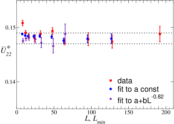
Figure 2: MC results $\bar{U}_{22}(L)$ and estimates of $\bar{U}_{22}^{*}(L_{\rm min})$ as obtained in different fits at fixed $R_{\xi}=0.5943$ for the RSIM at $p=0.8$. Some data are slightly shifted along the $x$-axis to make them visible. On the $x$ axis we report $L$ when plotting the MC data and the minimum lattice size $L_{\rm min}$ used in the fit when plotting the fit results. The dotted lines correspond to the final estimate $\bar{U}_{22}^{*}=0.148(1)$.

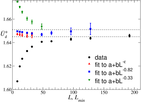
Figure 3: MC results $\bar{U}_{4}(L)$ and estimates of $\bar{U}_{4}^{*}(L_{\rm min})$ as obtained in different fits at fixed $R_{\xi}=0.5943$ for the RSIM at $p=0.8$. In the second fit ($a+bL^{-\epsilon}$) $\epsilon$ is a free parameter. As in Fig. 2, the $x$ axis corresponds to $L$ (MC data) and $L_{\rm min}$ (fit results). The dotted lines correspond to the final estimate $\bar{U}_{4}^{*}=1.648(3)$.

Here we determine the universal large-$L$ limits of the quartic cumulants $U_{22}$ and $U_{4}$ at fixed $R_{\xi}=0.5943$—we call them $\bar{U}_{22}$ and $\bar{U}_{4}$, respectively—using the data at $p=0.8$ reported in Table 2. The data of $\bar{U}_{22}$ in the range $8\leq L\leq 192$ shown in Fig. 2 have a very small $L$ dependence. In particular, there is no evidence of scaling corrections associated with the leading correction-to-scaling exponent $\omega\approx 0.3$. This confirms earlier results [18, 20, 19] indicating that leading scaling corrections in the RSIM at $p=0.8$ are very small. Moreover, also the next-to-leading scaling corrections associated with $\omega_{2}\approx 0.8$ are quite small. Indeed, if we fit the data with $L\geq L_{\rm min}$ to a constant, a fit with $\chi^{2}/{\rm DOF}\mathrel{\hbox to0.0pt{\lower 3.0pt\hbox{$\mathchar 536\relax$}\hss}\raise 2.0pt\hbox{$\mathchar 316\relax$}}1$ (DOF is the number of degrees of freedom of the fit) is already obtained for $L_{\rm min}=12$. The corresponding estimates of $\bar{U}_{22}^{*}$ are independent of $L_{\rm min}$ within error bars, see Fig. 2. We also fit the data to $a+bL^{-\epsilon}$ with $\epsilon=0.33$ and $\epsilon=0.82$, which are the best MC estimate of $\omega$ (see Sec. 5.3) and the FT estimate of $\omega_{2}$ (see A), respectively. In both cases $b\approx 0$ within errors already for $L_{\rm min}=16$. Finally, we also do fits keeping $\epsilon$ as a free parameter. The estimates of $\bar{U}_{22}^{*}$ are independent of $L_{\rm min}$ within error bars; for $L_{\rm min}=8$ we get $\bar{U}_{22}^{*}=0.1483(3)$, with $\chi^{2}/{\rm DOF}=0.8$. The estimates of $\bar{U}_{22}^{*}$ obtained in the fits with $\epsilon=0.82$ are also plotted in Fig. 2 versus the minimum lattice size $L_{\rm min}$ of the data considered in the fits. Collecting results, we obtain the final estimate

$$\bar{U}_{22}^{*}=0.148(1).$$ (30)

We perform a similar analysis of $\bar{U}_{4}$. The data are shown in Fig. 3. In this case, there is clear evidence of scaling corrections. A fit of the data to $a+bL^{-\epsilon}$, taking $\epsilon$ as a free parameter, gives $\bar{U}_{4}^{*}=1.6472(7)$ and $\epsilon=0.95(5)$ for $L_{\rm min}=8$: There is no evidence of scaling corrections with exponent $\omega\approx 0.3$. This is confirmed by fits to $a+bL^{-\epsilon}$ with $\epsilon=0.3$ fixed. The leading term $a$ varies significantly with $L_{\rm min}$, exactly as the original data (see Fig. 3). The numerical results for $\bar{U}_{4}$ are much better described by assuming that the leading scaling corrections are proportional to $L^{-\omega_{2}}\sim L^{-0.82}$. A fit to $a+bL^{-0.82}$ gives estimates of $\bar{U}_{4}^{*}$ that show a very tiny dependence on $L_{\rm min}$, see Fig. 3. The dependence on $\omega_{2}$ is also small: if $\omega_{2}$ varies between $0.74$ and $0.90$ [this corresponds to considering the FT estimate $\omega_{2}=0.82(8)$], estimates change by less than 0.001 for $L_{\rm min}\leq 32$. These analyses lead to the final estimate

$$\bar{U}_{4}^{*}=1.648(3).$$ (31)

We finally consider the difference $\bar{U}_{d}\equiv\bar{U}_{4}-\bar{U}_{22}$, whose data are very precise because of an unexpected cancellation of the statistical fluctuations, see Table 2. In Fig. 4 we show the results of the same fits as done for $\bar{U}_{4}$. They lead to the estimate

$$\bar{U}_{d}^{*}=1.500(1),$$ (32)

which is perfectly consistent with the estimates obtained for $\bar{U}_{22}^{*}$ and $\bar{U}_{4}^{*}$.

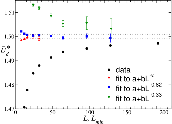
Figure 4: MC results $\bar{U}_{d}(L)$ and estimates of $\bar{U}_{d}^{*}(L_{\rm min})$ as obtained in different fits at fixed $R_{\xi}=0.5943$ for the RSIM at $p=0.8$. In the second fit ($a+bL^{-\epsilon}$) $\epsilon$ is a free parameter. As in Fig. 2, the $x$ axis corresponds to $L$ (MC data) and $L_{\rm min}$ (fit results). The dotted lines correspond to the final estimate $\bar{U}_{d}^{*}=1.500(1)$.

5.3 Estimate of the leading correction-to-scaling exponent $\omega$

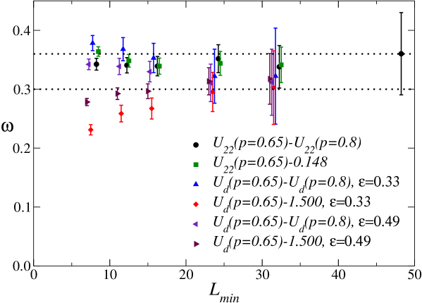
Figure 5: Estimates of $\omega$ from fits of $\Delta_{22,a}\equiv\bar{U}_{22}(p=0.65)-\bar{U}_{22}(p=0.8)$, $\Delta_{22,b}\equiv\bar{U}_{22}(p=0.65)-\bar{U}_{22}^{*}$, $\Delta_{d,a}\equiv\bar{U}_{d}(p=0.65)-\bar{U}_{d}(p=0.8)$, $\Delta_{d,b}\equiv\bar{U}_{d}(p=0.65)-\bar{U}_{d}^{*}$, as a function of $L_{\rm min}$, which is the minimum lattice size considered in the fits. $\Delta_{22,a}$ and $\Delta_{22,b}$ are fitted as $\ln\Delta=a-\omega\ln L$; $\Delta_{d,a}$ and $\Delta_{d,b}$ are fitted as $\ln\Delta=a-\omega\ln L+bL^{-\epsilon}$. Some data are slightly shifted along the $x$-axis to make them visible. The dotted lines correspond to the final estimate $\omega=0.33(3)$.

In order to estimate $\omega$, we use the data at $p=0.65$. We consider the differences

$$\Delta_{22,a}\equiv\bar{U}_{22}(p=0.65;L)-\bar{U}_{22}(p=0.8;L),$$ (33)

$$\Delta_{d,a}\equiv\bar{U}_{d}(p=0.65;L)-\bar{U}_{d}(p=0.8;L),$$ (34)

and also

$$\Delta_{22,b}\equiv\bar{U}_{22}(p=0.65;L)-\bar{U}_{22}^{*},$$ (35)

$$\Delta_{d,b}\equiv\bar{U}_{d}(p=0.65;L)-\bar{U}_{d}^{*},$$ (36)

where $\bar{U}_{22}^{*}$ and $\bar{U}_{d}^{*}$ are given in Eqs. (30) and (32). Because of the universality of the large-$L$ limit of the phenomenological couplings—hence, they do not depend on $p$—they behave as

$$\Delta\approx c_{\Delta,11}L^{-\omega}+c_{\Delta,12}L^{-2\omega}+\cdots+c_{\Delta,21}L^{-\omega_{2}}+\cdots$$ (37)

The quantities defined in Eqs. (33) and (35) are well fitted to $c_{\Delta,11}L^{-\omega}$. For instance, the analysis of $\Delta_{22,a}$ gives $\omega=0.342(10)$ and $\omega=0.352(24)$ for $L_{\rm min}=8$ and 24, respectively; in both cases $\chi^{2}/{\rm DOF}\approx 0.5$. Such a fit instead gives a relatively large $\chi^{2}/{\rm DOF}$ ($\chi^{2}/{\rm DOF}=2.3$ for $L_{\rm min}=12$) when applied to $\bar{U}_{d}$, essentially because the data of $\bar{U}_{d}$ have a better relative precision. Moreover, a clear systematic drift is observed when varying $L_{\rm min}$. Therefore, we must include the next-to-leading corrections. We thus performed fits of the form $c_{\Delta,11}L^{-\omega}(1+dL^{-\epsilon}$), where $\epsilon$ is an effective exponents that takes into account two next-to-leading corrections and should vary in $[\omega,\omega_{2}-\omega]$. Given the results obtained from the analysis of $\bar{U}_{22}$ and the FT estimate $\omega_{2}=0.82(8)$, we have taken $\epsilon\in[0.3,0.6]$. The dependence on $\epsilon$ is small: for instance, for $L_{\rm min}=16$, the analysis of $\Delta_{d,a}$ gives $\omega=0.35(3)$, 0.33(2), 0.32(2) for $\epsilon=0.3$, 0.5, 0.6. The results corresponding to $\epsilon=0.33$ and $\epsilon=0.49\approx\omega_{2}-\omega$ are reported in Fig. 5 as a function of $L_{\rm min}$, the smallest lattice size used in the analysis. They lead to the estimate

$$\omega=0.33(3),$$ (38)

which is in agreement with the FT six-loop result [11] $\omega=0.25(10)$ (we also mention the five-loop result $\omega=0.32(6)$ of Ref. [12]) and with the MC result [18] $\omega=0.37(6)$.

In writing Eq. (37) we assumed that the scaling limit does not depend on $p$. We can now perform a consistenty check, verifying whether $\bar{U}_{22}$ and $\bar{U}_{4}$ for $p=0.65$ converge to the estimates (30) and (31). A fit of $\bar{U}_{22}$ to $\bar{U}_{22}^{*}+c_{22,11}L^{-\omega}+c_{22,2}L^{-\epsilon}$ gives $\bar{U}_{22}^{*}=0.154(4)$, 0.152(2), 0.149(6), 0.148(5) for $(L_{\rm min},\epsilon)=(8,2\omega)$, $(8,\omega_{2})$, $(12,2\omega)$, $(12,\omega_{2})$, respectively. Here we used $\omega=0.33$ as determined above and $\omega_{2}=0.82$. These results are in agreement with the estimate (30). Such an agreement is also clear from Fig. 6, where we plot $\bar{U}_{22}$ versus $L^{-\omega}$. The same analysis applied to $\bar{U}_{4}$ gives $\bar{U}_{4}^{*}=1.640(4)$, 1.644(3), 1.640(5), 1.644(4), for the same values of $(L_{\rm min},\epsilon)$, which are compatible with the estimate (31).

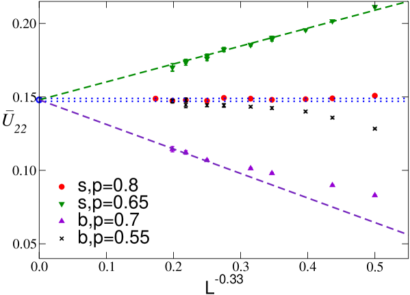
Figure 6: Plot of $\bar{U}_{22}$ versus $L^{-\omega}$ with $\omega=0.33$ for the RSIM (s) at $p=0.8$ and $p=0.65$ and for the RBIM (b) at $p=0.7$ and $p=0.55$.

5.4 Determination of the improved RSIM

We now estimate the value $p^{*}$ of the spin concentration that corresponds to an improved model: for $p=p^{*}$ the leading scaling corrections with exponent $\omega$ vanish. We already know that the RSIM with $p=0.8$ is approximately improved, so that $p^{*}\approx 0.8$. In the following we make this statement more precise. We consider $\bar{U}_{22}$, which has small next-to-leading scaling corrections, and determine the value of $p$ at which the leading scaling corrections to this quantity vanish. As we remarked in Sec. 3.1, the same cancellation occurs in any other quantity.

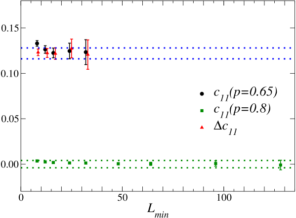
Figure 7: Results of the fits to estimate the amplitude of the leading scaling correction in $\bar{U}_{22}$.

To determine $p^{*}$, we fit the data of $\bar{U}_{22}$ at $p=0.8$ and $p=0.65$ to $\bar{U}_{22}^{*}+c_{22,11}(p)L^{-\epsilon}$, and the difference $\Delta_{22,a}$ defined in Eq. (33) to $c_{\Delta,11}L^{-\epsilon}$. We have performed fits in which $\epsilon$ is fixed, $\epsilon=\omega=0.33(3)$, and fits in which it is taken as a free parameter. The results of the fits with $\epsilon=\omega$ are shown in Fig. 7 for several values of $L_{\rm min}$, the smallest lattice size included in the fit. We obtain

$$c_{\Delta,11}=0.122(6),$$

$$c_{22,11}(p=0.65)=0.122(6),$$ (39)

$$c_{22,11}(p=0.8)=0.000(4),$$

where the first two estimates correspond to $L_{\rm min}=16$ and the last one to $L_{\rm min}=48$; errors are such to include the results of all fits. These results give us the upper bound

$$\left|{c_{22,11}(p=0.8)\over c_{22,11}(p=0.65)}\right|\mathrel{\hbox to0.0pt{\lower 3.0pt\hbox{$\mathchar 536\relax$}\hss}\raise 2.0pt\hbox{$\mathchar 316\relax$}}{4\over 122}\approx{1\over 30}.$$ (40)

For $p=0.8$ scaling corrections are at least a factor of 30 smaller than those occurring for $p=0.65$. This bound will be useful in the following to assess the relevance of the “systematic error” in the fits of the data at $p=0.8$ due to possible residual leading scaling corrections. Indeed, the ratio that appears in Eq. (40) does not depend on the observable. In the notations of Sec. 3, $c_{22,11}(p)=r_{3,0}(z_{f})u_{3}(t=0,p)$ where $r_{3,0}(z_{f})$ is a model-independent constant that depends on the observable (in this case on $\bar{U}_{22}$). The constant $r_{3,0}(z_{f})$ drops out in the ratio, since

$${c_{22,11}(p_{1})\over c_{22,11}(p_{2})}={u_{3}(t=0,p_{1})\over u_{3}(t=0,p_{2})}.$$ (41)

Therefore, given a generic observable ${\cal O}(p)$ that behaves as

$${\cal O}(p)=a(p)L^{\sigma}(1+c_{{\cal O},11}(p)L^{-\omega}+\ldots),$$ (42)

we have in all cases

$$|c_{{\cal O},11}(p=0.8)/c_{{\cal O},11}(p=0.65)|\mathrel{\hbox to0.0pt{\lower 3.0pt\hbox{$\mathchar 536\relax$}\hss}\raise 2.0pt\hbox{$\mathchar 316\relax$}}1/30.$$ (43)

Estimates (39) allow us to estimate $p^{*}$. We obtain $p^{*}\approx 0.80$. Since, $c_{22,11}(p)=a(p-p^{*})$ close to $p\approx 0.80$, the error on $p^{*}$ is simply ${\rm err}[c_{22,11}(p=0.8)]/|a|$. The constant $a$—we only need a rough estimate since it is only relevant for the error on $p^{*}$—is determined as

$$a=\left.{dc_{22,11}\over dp}\right|_{p=p^{*}}\approx{c_{22,11}(p=0.8)-c_{22,11}(p=0.65)\over 0.8-0.65}=-0.81(4),$$ (44)

where the reported error is obtained from those of $c_{22,11}(p=0.8)$ and $c_{22,11}(p=0.65)$. This gives

$$p^{*}=0.800(5).$$ (45)

We are not able to assess the error on $a$ due to the approximation (44). Note, however, that the dependence on $a$ is small. If we vary $a$ by a factor of 2, $p^{*}$ changes at most by 0.01.

5.5 Determination of the critical temperatures

We determine the critical temperature by extrapolating the estimates of $\beta_{f}$ reported in Tables 1 and 3. According to the discussion reported in Sec. 3, since we have chosen $R_{\xi}=0.5943\approx R_{\xi}^{*}$, we expect in general that $\beta_{f}-\beta_{c}=O(L^{-1/\nu-\omega})$. For $p=0.8$, since the model is improved, the leading scaling corrections are related to the next-to-leading exponent $\omega_{2}$. Thus, in this case $\beta_{f}-\beta_{c}=O(L^{-1/\nu-\omega_{2}})$

In Fig. 8 we show the data for $p=0.8$ versus $L^{-1/\nu-\omega_{2}}$ taking $\nu=0.68$ and $\omega_{2}=0.82$. The expected linear behavior is clearly observed. A fit to $\beta_{c}+cL^{-1/\nu-\omega_{2}}$ gives $\beta_{c}=0.2857429(4)$. We have also taken into account the error on $\omega_{2}$ and on $\nu$ (the error due to the variation of $\nu$ is essentially negligible compared to the first one). This result improves the estimate of $\beta_{c}$ obtained in Ref. [19], i.e. $\beta_{c}=0.285744(2)$.

For $p=0.65$ we fit $\beta_{f}$ to $\beta_{c}+cL^{-1/\nu-\omega}+dL^{-1/\nu-\epsilon}$ with $\nu=0.68$, $\omega=0.33(3)$, $\epsilon\in[0.6,0.9]$. We obtain $\beta_{c}=0.370174(3)$. This is consistent with the estimate $\beta_{c}=0.370166(6)$ ($L_{\rm min}=16$) reported in Ref. [18].

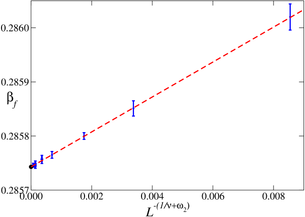
Figure 8: Estimates of $\beta_{f}$ for $p=0.8$ versus $L^{-(1/\nu+\omega_{2})}$, for $\omega_{2}=0.82$ and $\nu=0.68$. The dashed line corresponds to a linear fit of the data.

5.6 Improved phenomenological couplings

Beside considering improved Hamiltonians—in these particular models any thermodynamic quantity does not have leading scaling corrections—one may also consider improved observables which are such that the leading scaling correction vanishes for any Hamiltonian. Here we determine an improved phenomenological coupling by taking an appropriate combination of the cumulants $\bar{U}_{4}$ and $\bar{U}_{22}$, i.e. we consider

$$\bar{U}_{\rm im}\equiv\bar{U}_{4}+c_{\rm im}\bar{U}_{22}.$$ (46)

In the scaling limit we have generically $\bar{U}_{\#}\approx\bar{U}_{\#}^{*}+c_{\#,11}L^{-\omega}$. The constant $c_{\rm im}$ is determined by requiring $c_{{\rm im},11}=0$, which gives

$$c_{\rm im}=-{c_{4,11}(p)\over c_{22,11}(p)},$$ (47)

where we have written explicitly the $p$ dependence of the coefficients $c_{4,11}(p)$ and $c_{22,11}(p)$. As discussed in Sec. 3.1, the ratio (47) is universal within the RDIs universality class and, in particular, independent of $p$. Indeed, $c_{4,11}=r_{U_{4},3,0}(z_{f})u_{3}$, $c_{22,11}=r_{U_{22},3,0}(z_{f})u_{3}$, where $r_{U_{4},3,0}(z)$ and $r_{U_{22},3,0}(z)$ are the universal scaling functions defined in Sec. 3.1. The model-dependent scaling field $u_{3}$ cancels out in the ratio, proving its universality. The combination $\bar{U}_{\rm im}$ with the choice (47) has no leading scaling corrections associated with the exponent $\omega$, so that, see Sec. 3.1, $\bar{U}_{\rm im}=\bar{U}_{\rm im}^{*}+O(L^{-2\omega},L^{-\omega_{2}})$.

The ratio $c_{\rm im}$ can be estimated by determining the leading scaling correction amplitudes of $\bar{U}_{22}$ and $\bar{U}_{4}$. Alternatively, one may estimate it from the ratio

$${\bar{U}_{4}(p=0.65;L)-\bar{U}_{4}(p=0.8;L)\over\bar{U}_{22}(p=0.65;L)-\bar{U}_{22}(p=0.8;L)}=-c_{\rm im}+aL^{-\omega}+bL^{-\omega_{2}+\omega}+\cdots$$ (48)

Both analyses give consistent results, leading to the estimate

$$c_{\rm im}=1.3(1).$$ (49)

Therefore,

$$\bar{U}_{\rm im}=\bar{U}_{4}+1.3\bar{U}_{22}$$ (50)

has (approximately) vanishing leading scaling corrections for any model and any $p$. More precisely, we have the upper bound $|c_{{\rm im},11}|\mathrel{\hbox to0.0pt{\lower 3.0pt\hbox{$\mathchar 536\relax$}\hss}\raise 2.0pt\hbox{$\mathchar 316\relax$}}0.1|c_{22,11}|$. Since $c_{4,11}=-c_{\rm im}c_{22,11}$ and $c_{d,11}=-(1+c_{\rm im})c_{22,11}$, we also have $|c_{{\rm im},11}|\mathrel{\hbox to0.0pt{\lower 3.0pt\hbox{$\mathchar 536\relax$}\hss}\raise 2.0pt\hbox{$\mathchar 316\relax$}}0.1|c_{4,11}|$ and $|c_{{\rm im},11}|\mathrel{\hbox to0.0pt{\lower 3.0pt\hbox{$\mathchar 536\relax$}\hss}\raise 2.0pt\hbox{$\mathchar 316\relax$}}0.05|c_{d,11}|$. The leading scaling corrections in $\bar{U}_{\rm im}$ are at least a factor of 10 smaller than those occurring in $\bar{U}_{22}$ and $\bar{U}_{4}$ and a factor of 20 smaller than those occurring in $\bar{U}_{d}$. This is confirmed by a direct analysis of the data of $\Delta_{{\rm im},b}$, defined as in Eq. (35), at $p=0.65$. A fit to $c_{{\rm im},11}L^{-\omega}$, $\omega=0.33$, gives $|c_{{\rm im},11}|\mathrel{\hbox to0.0pt{\lower 3.0pt\hbox{$\mathchar 536\relax$}\hss}\raise 2.0pt\hbox{$\mathchar 316\relax$}}0.005$, to be compared with $c_{22,11}=0.122(6)$ obtained in Sec. 5.3. In Fig. 9 we show results of fits of $\bar{U}_{\rm im}$ to $\bar{U}_{\rm im}^{*}+cL^{-\epsilon}$ with $\epsilon=0.66\approx 2\omega$ and $\epsilon=0.82\approx\omega_{2}$. They are consistent with the estimate $\bar{U}_{\rm im}^{*}=1.840(4)$, which can be obtained from the estimates of $\bar{U}_{4}$, $\bar{U}_{22}$, and $\bar{U}_{d}$ obtained in Sec. 5.2. The improved quantity $\bar{U}_{\rm im}$ is particularly useful to check universality, because it is less affected by scaling corrections.

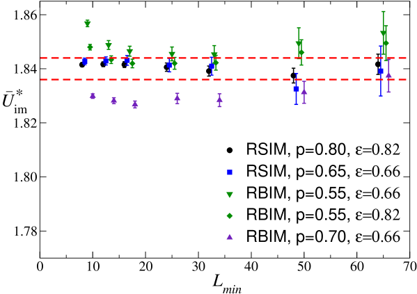
Figure 9: Estimates of $\bar{U}_{\rm im}^{*}$ obtained from fits of $\bar{U}_{\rm im}$ to $\bar{U}_{\rm im}^{*}+bL^{-\epsilon}$. The dashed lines correspond to the estimate $\bar{U}_{\rm im}^{*}=1.840(4)$ obtained from fits of $\bar{U}_{4}$, $\bar{U}_{22}$, $\bar{U}_{d}$ at $p=0.8$.

We should note that $\bar{U}_{\rm im}$ is useful in generic models in which $L^{-\omega}$ corrections are generically present, but is not the optimal quantity in improved models in which the leading scaling corrections are proportional to $c_{21}L^{-\omega_{2}}$. The coefficients $c_{21}$ can be estimated from the data at $p=0.8$, obtaining

$$c_{22,21}=0.01(2),$$

$$c_{4,21}=-0.21(5),$$

$$c_{d,21}=-0.22(5),$$

$$c_{{\rm im},21}=-0.20(5).$$ (51)

Since the ratios $c_{a,21}/c_{b,21}=r_{a,4,0}(z_{f})/r_{b,4,0}(z_{f})$ are universal, the coefficient $c_{22,21}$ is at least a factor of 5 smaller than the corresponding one in $\bar{U}_{\rm im}$, $\bar{U}_{4}$, $\bar{U}_{d}$ in any RDIs model. Hence, in improved models $\bar{U}_{22}$ and not $\bar{U}_{\rm im}$ is the optimal quantity.

5.7 The critical exponent $\nu$

We estimate the critical exponent $\nu$ by using the data at $p=0.8$, since in this case there are no leading corrections to scaling—the model is improved—the data have smaller errors, and we have results for larger lattices. We analyze the derivatives $R_{\xi}^{\prime}$ and $U_{4}^{\prime}$ at fixed $R_{\xi}$.

Since we have established that the RSIM at $p=0.8$ is improved, the dominant scaling corrections are associated with the next-to-leading exponent $\omega_{2}$. Therefore, we fit $R^{\prime}$ to $aL^{1/\nu}$ and to

$$aL^{1/\nu}\left(1+cL^{-\omega_{2}}\right)$$ (52)

or, more precisely, $\ln R^{\prime}$ to $\ln a+{1\over\nu}\ln L$ or to $\ln a+{1\over\nu}\ln L+cL^{-\omega_{2}}$. The exponent $\omega_{2}$ is fixed to the FT value $\omega_{2}=0.82(8)$. The results are reported in Fig. 10 as a function of $L_{\rm min}$. These fits are quite good, with $\chi^{2}/{\rm DOF}\mathrel{\hbox to0.0pt{\lower 3.0pt\hbox{$\mathchar 536\relax$}\hss}\raise 2.0pt\hbox{$\mathchar 316\relax$}}1$ already for relatively smal values of $L_{\rm min}$. The dependence on $\omega_{2}$ is negligible when $\omega_{2}$ varies within the range allowed by the FT estimate. The fits of $R^{\prime}_{\xi}$ to a simple power law are quite stable. The results for $L_{\rm min}\geq 48$ provide the estimate

$$\nu=0.6835(10).$$ (53)

The exponent $\nu$ can also be determined by analyzing the ratio ${\chi^{\prime}/\chi}$, where $\chi^{\prime}$ is the derivative of $\chi$ with respect to $\beta$. This ratio also has the asymptotic behavior (52). The corresponding results are in perfect agreement with those obtained by using $R^{\prime}_{\xi}$ and $U^{\prime}_{4}$.

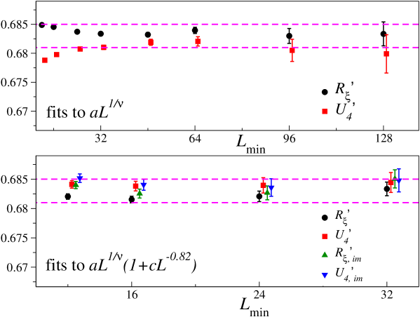
Figure 10: Estimates of the critical exponent $\nu$, obtained by fitting the MC data for the RSIM at $p=0.8$ to a simple power law (above), i.e. to $aL^{1/\nu}$, and to Eq. (52) with $\omega_{2}=0.82$. We consider $R_{\xi}^{\prime}$, $U_{4}^{\prime}$, $R^{\prime}_{\xi,{\rm im}}$ and $U^{\prime}_{4,{\rm im}}$. Some results are slightly shifted along the $x$-axis to make them visible. The dotted lines correspond to the final estimate $\nu=0.683(2)$.

Collecting results we obtain the final estimate

$$\nu=0.683(2),$$ (54)

which takes into account the fits of $R^{\prime}_{\xi}$ and $U^{\prime}_{4}$, with and without the scaling correction with exponent $\omega_{2}$. In the determination of the estimate (54), we have implicitly assumed that the RSIM at $p=0.8$ is exactly improved so that there are no leading scaling corrections. However, $p^{*}$ is only known approximately and thus some residual leading scaling corrections may still be present. To determine their relevance, we use the upper bound (43) and the MC results for $R^{\prime}$ at $p=0.65$. If the leading scaling corrections do not vanish, $R^{\prime}$ behaves as

$$R^{\prime}=aL^{1/\nu}\left(1+b_{R^{\prime},11}L^{-\omega}+b_{R^{\prime},12}L^{-2\omega}+b_{R^{\prime},21}L^{-\omega_{2}}+\cdots\right)\;.$$ (55)

In the following section we obtain the estimates

$$b_{R^{\prime}_{\xi},11}(p=0.65)=0.60(15),\qquad\qquad b_{U^{\prime}_{4},11}(p=0.65)=0.40(15).$$ (56)

Bound (43) gives then $|b_{R^{\prime},11}(p=0.80)|\mathrel{\hbox to0.0pt{\lower 3.0pt\hbox{$\mathchar 536\relax$}\hss}\raise 2.0pt\hbox{$\mathchar 316\relax$}}0.02$ for both $R^{\prime}_{\xi}$ and $U^{\prime}_{4}$. We have thus repeated the analysis at $p=0.8$ considering $R^{\prime}/(1\pm 0.02L^{-\omega})$, with $\omega=0.33$. The results for the exponent $\nu$ vary by $\pm 0.0004$, which is negligible with respect to the final error quoted in Eq. (54).

The result (54) is in agreement with and improves earlier MC estimates: $\nu=0.683(3)$ (Ref. [19]) and $\nu=0.6837(53)$ (Ref. [18]). It is also in agreement with the FT result [11] $\nu=0.678(10)$.

To check universality, it is interesting to compute $\nu$ directly, using the data at $p=0.65$. We fitted $\ln R^{\prime}$ to $a+(1/\nu)\ln L+cL^{-\omega}+dL^{-\epsilon}$ taking $\omega=0.33(3)$ and $\epsilon\in[0.6,0.9]$ (as before the last term takes into account corrections of order $L^{-2\omega}$ and $L^{-\omega_{2}}$). We obtain $\nu=0.65(2)$, $0.67(2)$, $0.68(2)$ for $L_{\rm min}=8,12,16$. The somewhat large error is mainly due to the variation of the estimate with $\epsilon$. Thus, if scaling corrections are taken into account, universality is satisfied.

5.8 Improved estimators for the critical exponent $\nu$

As we did in Sec. 5.6 for the phenomenological couplings, we wish now to define improved estimators of the critical exponent $\nu$, i.e., quantities $R^{\prime}_{\rm im}$ such that $b_{R^{\prime}_{\rm im},11}=0$, see Eq. (55). We will again combine data at $p=0.8$ with data at $p=0.65$.

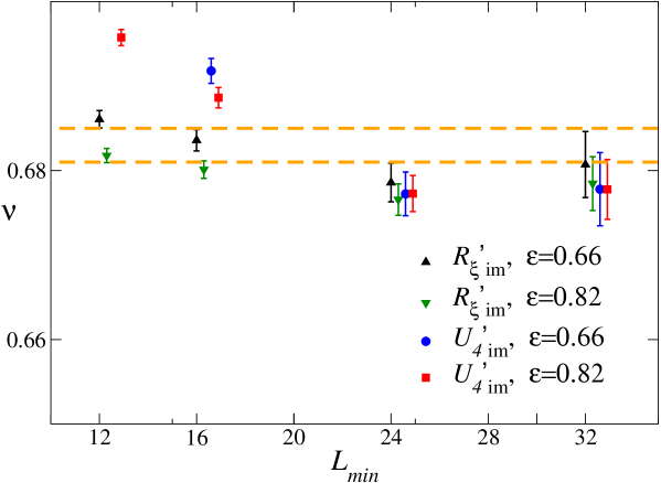
Figure 11: Results of fits to $aL^{1/\nu}(1+cL^{-\epsilon})$ of $R^{\prime}_{\xi,{\rm im}}$ and $U^{\prime}_{4,{\rm im}}$ for the RSIM at $p=0.65$. Some results are slightly shifted along the $x$-axis to make them visible. The dashed lines correspond to the estimate $\nu=0.683(2)$ obtained from the analysis of the data at $p=0.8$.

Let us consider a phenomenological coupling. In the following we choose $\bar{U}_{d}$ defined in Eq. (17) because it has the least relative statistical errors among the combinations of $\bar{U}_{4}$ and $\bar{U}_{22}$. For generic values of $p$ it has the asymptotic behavior

$$\bar{U}_{d}(p;L)=\bar{U}_{d}^{*}\left(1+\bar{c}_{d,11}(p)L^{-\omega}+\cdots\right).$$ (57)

Analyzing the data as described in Secs. 5.2 and 5.3, we obtain the estimate $\bar{c}_{d,11}(p=0.65)=-0.16(2)$. Then, given a generic coupling $R^{\prime}$ with asymptotic behavior (55), we have

$${R^{\prime}(p=0.65;L)\over R^{\prime}(p=0.8;L)}=A\left(1+\Delta b_{R^{\prime},11}L^{-\omega}+\cdots\right),$$ (58)

where $\Delta b_{R^{\prime},11}=b_{R^{\prime},11}(p=0.65)-b_{R^{\prime},11}(p=0.8)$. A fit of the MC data to Eq. (58) gives $\Delta b_{R^{\prime}_{\xi},11}=0.60(15)$ and $\Delta b_{U_{4}^{\prime},11}=0.40(15)$. Bound (43) implies $|b_{R^{\prime},11}(p=0.8)|\mathrel{\hbox to0.0pt{\lower 3.0pt\hbox{$\mathchar 536\relax$}\hss}\raise 2.0pt\hbox{$\mathchar 316\relax$}}|b_{R^{\prime},11}(p=0.65)|/30$. Therefore, given the error bars on the previous results, we can identify $\Delta b_{R^{\prime},11}$ with $b_{R^{\prime},11}(p=0.65)$, obtaining the estimates already reported in Eq. (56). Finally we consider

$$R^{\prime}_{\rm im}=R^{\prime}\bar{U}_{d}^{a}\sim L^{1/\nu}[1+(b_{R^{\prime},11}+a\bar{c}_{d,11})L^{-\omega}+\cdots]\;.$$ (59)

If we fix $a=-b_{R^{\prime},11}/\bar{c}_{d,11}$, the quantity $R^{\prime}_{\rm im}$ is improved. Using the results obtained above, we find that

$$R^{\prime}_{\xi,{\rm im}}\equiv R^{\prime}_{\xi}\bar{U}_{d}^{a_{\xi}}\quad{\rm with}\quad a_{\xi}=4(1),$$ (60)

$$U^{\prime}_{4,{\rm im}}\equiv U^{\prime}_{4}\bar{U}_{d}^{a_{u}}\quad{\rm with}\quad a_{u}=2.5(1.0)$$ (61)

are approximately improved quantities. As a check of the results, we perform the fits (58) also for the improved observables. In both cases $\Delta b_{R^{\prime},11}$ is consistent with zero.

At $p=0.8$ these improved quantities give results which are substantially equivalent to those of the original quantities, as shown in Fig. 10, where we report the estimates corresponding to the central values of the exponents $a_{\xi}$ and $a_{u}$. This is not unexpected, since the RSIM at $p=0.8$ has suppressed leading scaling correction for any quantity.

The use of the improved estimators is particularly convenient at $p=0.65$. Indeed, as discussed in the previous Section, the direct analysis of $R^{\prime}_{\xi}$ and $U^{\prime}_{4}$ gives estimates of $\nu$ with a large error. In the improved quantities $R^{\prime}_{\xi,{\rm im}}$ and $U^{\prime}_{4,{\rm im}}$ the leading scaling correction is absent and thus one should be able to determine more precise estimates of $\nu$ and perform a more severe consistency check of universality. Since $b_{R^{\prime},11}=0$, we fit the data to

$$R^{\prime}_{\rm im}=aL^{1/\nu}\left(1+cL^{-\epsilon}\right)$$ (62)

with $\epsilon\in[0.6,0.9]$. The results of these fits are shown in Fig. 11 (we report results corresponding to the two choices $\epsilon=0.66\approx 2\omega$ and $\epsilon=0.82\approx\omega_{2}$). Explicitly, we find $\nu=0.687(7)$, 0.684(7), 0.679(6), 0.680(8) from the analysis of $R^{\prime}_{\xi,{\rm im}}$ with $L_{\rm min}=12$, 16, 24, 32. The error includes the statistical error, the error on $a_{\xi}$, and the variation of the estimate with $\epsilon$. The results for $U^{\prime}_{4,\rm im}$ are perfectly consistent. The estimates are three times more precise than those obtained by using the unimproved $R_{\xi}^{\prime}$ and $U_{4}^{\prime}$ and are in good agreement with the more precise estimate $\nu=0.683(2)$ obtained from the data at $p=0.8$.

5.9 Estimate of the critical exponent $\eta$

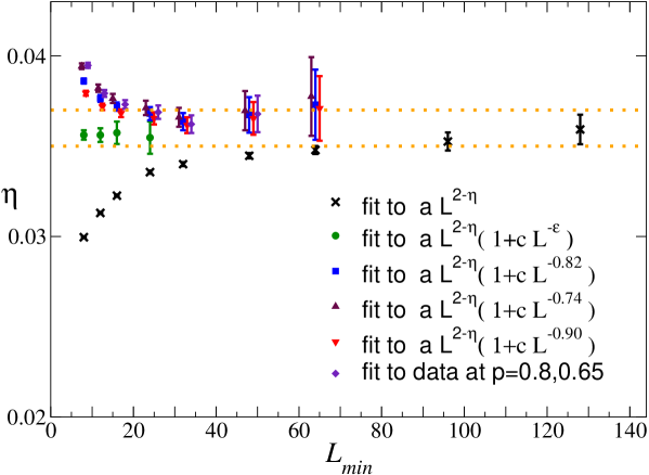
Figure 12: Estimates of the critical exponent $\eta$, obtained by fitting the magnetic susceptibility $\chi$. All fits refer to the RSIM at $p=0.8$, except the last one where we simultaneously fit data at $p=0.8$ and at $p=0.65$ (see text). Some results are slightly shifted along the $x$-axis to make them visible. The dotted lines correspond to the final estimate $\eta=0.036(1)$.

In order to estimate the critical exponent $\eta$ we analyze the magnetic susceptibility $\chi$. We have fitted the data at $p=0.8$ to $aL^{2-\eta}$, to $aL^{2-\eta}(1+cL^{-\epsilon})$, taking $\epsilon$ as a free parameter, and to $aL^{2-\eta}(1+cL^{-\omega_{2}})$ with $\omega_{2}=0.82,0.74,0.90$ [we use, as before, the FT estimate $\omega_{2}=0.82(8)$]. Moreover, we simultaneously fit the data at $p=0.8$ and $p=0.65$ to $a_{1}L^{2-\eta}(1+c_{1}L^{-0.82})$ if $p=0.8$ and $a_{2}L^{2-\eta}(1+c_{2}L^{-0.33})$ if $p=0.65$. The results are shown in Fig. 12. They are fully consistent and provide the final estimate

$$\eta=0.036(1).$$ (63)

Again we should discuss the error due to possible residual leading scaling corrections at $p=0.8$. A fit of the data at $p=0.65$ to $aL^{2-\eta}(1+cL^{-\omega_{2}})$ gives $\eta\approx 0.035$. Even if we neglect the correction term proportional to $L^{-\omega}$, the result of the fit is compatible with the estimate (63). This means that the amplitude of $L^{-\omega}$ is quite small for $p=0.65$ and gives a correction of the order of the statistical error in Eq. (63). The amplitude of $L^{-\omega}$ at $p=0.8$ is at least 30 times smaller, see Eq. (43). Therefore, residual scaling corrections are negligible.

The result (63) improves earlier estimates: $\eta=0.035(2)$ and $\eta=0.0374(45)$ from MC simulations of Refs. [19] and [18] respectively. It is also close to, though not fully compatible with, the FT result $\eta=0.030(3)$ [11].

6 Finite-size scaling analysis of the random site-diluted Ising model at fixed $\beta$

In this section we perform a different analysis using the results at $\beta=\beta_{\rm run}$ (the value of $\beta$ at which we performed the MC simulation) for the RSIM at $p=0.8$. Thus, the data we use here are different from those considered in the previous Section. We will combine them with those obtained close to the critical point ($0.28572\leq\beta\leq 0.28578$) in Ref. [19]. The statistics of the old results is comparable with that obtained here for $p=0.8$; note however that we have now also results for the larger lattice size $L=192$.

6.1 Phenomenological couplings and critical temperature

$L_{\rm min}$	$\beta_{c}$	$U_{4}^{*}$	$U_{22}^{*}$	$R_{\xi}^{*}$	$\epsilon$
8	0.2857432(3)	1.6476(10)	0.14779(26)	0.59394(23)	0.97(7)
12	0.2857432(3)	1.6480(15)	0.14791(32)	0.59393(30)	0.94(13)
16	0.2857430(3)	1.6480(18)	0.14787(35)	0.59363(32)	0.97(18)
24	0.2857434(4)	1.6471(27)	0.14801(51)	0.59427(66)	0.99(45)
8	0.2857430(3)[1]	1.6499(5)[16]	0.14761(29)[13]	0.59410(26)[11]	fixed
12	0.2857430(3)[1]	1.6494(6)[13]	0.14781(33)[9]	0.59403(31)[8]	fixed
16	0.2857429(3)[1]	1.6497(7)[12]	0.14775(37)[9]	0.59370(36)[5]	fixed
24	0.2857433(4)[1]	1.6482(12)[7]	0.14793(55)[5]	0.59444(64)[10]	fixed
32	0.2857436(5)[1]	1.6472(14)[6]	0.14768(61)[7]	0.59494(74)[14]	fixed

Table 6: Results of the combined fits for the phenomenological couplings for several values of $L_{\rm min}$, the smallest lattice size used in the analyses. In the first set of fits, $\epsilon$ is free, while in the second set we fixed $\epsilon=\omega_{2}=0.82(8)$. The number in parentheses is the statistical error, while the number in brackets gives the variation of the estimate as $\omega_{2}$ is varied within one error bar.

As discussed in Sec. 3.1, close to the critical point a phenomenological coupling behaves as [see Eq. (23)]

$$R(\beta,L)=R^{*}+a_{1}(\beta-\beta_{c})L^{1/\nu}+a_{2}L^{-\epsilon}.$$ (64)

In order to determine $R^{*}$ and $\beta_{c}$ we have performed two different types of fit, always fixing $\nu=0.683(5)$ [results are essentially unchanged if we vary $\nu$ in $[0.678,0.688]$, which is quite conservative given the estimate (54)]. In the first case, we simultaneously fit $R_{\xi}$, $U_{4}$, and $U_{22}$, keeping $\epsilon$ as a free parameter. For the exponent $\epsilon$ we obtain $\epsilon=0.95(20)$: as expected there is no indication of a correction-to-scaling term with exponent $\omega\approx 0.33$. In the second fit, we use the fact that the model is improved, set $\epsilon=\omega_{2}$, and use the FT estimate $\omega_{2}=0.82(8)$. The results of the fits for several values of $L_{\rm min}$ are reported in Table 6. They are quite stable with respect to $L_{\rm min}$ and indeed results with $L_{\rm min}=8$ are compatible with all those that correspond to larger values. If we take conservatively the final estimates from the results with $L_{\rm min}=24$ and $\omega_{2}$ fixed, we have

$$\beta_{c} = 0.2857433(5),$$

$$R^{*}_{\xi} = 0.5944(7),$$

$$U^{*}_{4} = 1.648(2),$$

$$U^{*}_{22} = 0.1479(6).$$ (65)

The estimate of $\beta_{c}$ is compatible with that reported in Sec. 5.5, $\beta_{c}=0.2857429(4)$. The estimate of $R^{*}_{\xi}$ is essentially identical to that reported in Ref. [19], $R^{*}_{\xi}=0.5943(9)$, so that our analysis at fixed $R_{\xi}=0.5943$ corresponds indeed to fixing $R_{\xi}=R^{*}_{\xi}$. This is also confirmed by the results for $U^{*}_{4}$ and $U^{*}_{22}$ that are compatible with the estimates of $\bar{U}^{*}_{4}$ and $\bar{U}^{*}_{22}$ obtained in Sec. 5.2 (if we had performed analyses at fixed $R_{\xi}\not=R^{*}_{\xi}$ such an equality would not hold, see Sec. 3.2). The estimates of ${U}^{*}_{4}$ and ${U}^{*}_{22}$ agree with previous MC estimates: $U^{*}_{4}=1.650(9)$ and $U^{*}_{22}=0.1480(10)$ (Ref. [19]); $U^{*}_{4}=1.653(20)$ and $U^{*}_{22}=0.145(7)$ (Ref. [18]).

6.2 Estimates of $\nu$

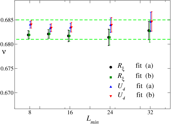
Figure 13: Estimates of the critical exponent $\nu$, obtained by simultaneous fits of $R_{\xi}$ and $R^{\prime}_{\xi}$, and of $U_{4}$ and $U^{\prime}_{4}$ (see text). Some results are slightly shifted along the $x$-axis to make them visible. The dashed lines correspond to the estimate $\nu=0.683(2)$ obtained in Sec. 5.7.

We now compute the critical exponent $\nu$. It may be obtained by fitting $R^{\prime}(\beta=\beta_{c},L)$ to $aL^{1/\nu}$. This requires fixing $\beta_{c}$ and this induces a somewhat large error. We have found more convenient to follow a different route, analyzing simultaneously $R^{\prime}$ (this gives $\nu$) and $R$ (this essentially fixes $\beta_{c}$). We performed two types of fits. First [fit (a)], we fit $R$ and $R^{\prime}$ to

$$R(\beta,L) = R^{*}+a_{1}(\beta-\beta_{c})L^{1/\nu}+a_{2}L^{-\epsilon}$$

$$\qquad+a_{3}(\beta-\beta_{c})^{2}L^{2/\nu}+a_{4}(\beta-\beta_{c})L^{1/\nu-\epsilon},$$

$$R^{\prime}(\beta,L) = a_{1}L^{1/\nu}+2a_{3}(\beta-\beta_{c})L^{2/\nu}+a_{4}L^{1/\nu-\epsilon}.$$ (66)

Here $\beta_{c}$ and $\nu$ are kept as free parameters, while $\epsilon$ is fixed: $\epsilon=\omega_{2}=0.82(8)$. In the second fit [fit (b)], we fit $R$ and $R^{\prime}$ to

$$R(\beta,L)=R^{*}+a_{1}(\beta-\beta_{c})L^{1/\nu}+a_{2}L^{-\epsilon},$$

$$\ln[R^{\prime}(\beta,L)]=a_{3}+{1\over\nu}\ln L+a_{4}(\beta-\beta_{c})L^{1/\nu}+a_{5}L^{-\epsilon},$$ (67)

where again $\epsilon=\omega_{2}=0.82(8)$. The two fits give similar results, see Fig. 13. For instance, for $L_{\rm min}=24$ and $R=R_{\xi}$ we have $\nu=0.6814(17)$ and 0.6814(16) from fit (a) and (b), respectively (the reported errors are the sum of the statistical error and of the variation of the estimate as $\omega_{2}$ is varied within one error bar). If $R=U_{4}$ we obtain analogously $\nu=0.6839(15)$ and 0.6840(16). Collecting results, this type of analysis gives the final estimate

$$\nu=0.6825(25),$$ (68)

which is fully compatible with Eq. (54).

6.3 Estimates of $\eta$

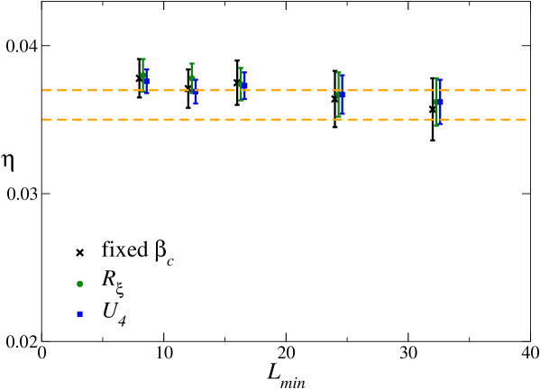
Figure 14: Estimates of the critical exponent $\eta$, obtained in different fits (see text). Some results are slightly shifted along the $x$-axis to make them visible. The dashed lines correspond to the estimate $\eta=0.036(1)$ obtained in Sec. 5.9.

As in Ref. [19] we determine $\eta$ from the critical behavior of $Z\equiv\chi/\xi^{2}$, which is more precise than $\chi$: The relative error on $\chi$ is 3.4 times larger than the relative error on $Z$. We perform two types of fits. First, we analyze $Z$ as

$$\ln[Z(\beta,L)]=a-\eta\ln L+bL^{1/\nu}(\beta-\beta_{c})+cL^{-\omega_{2}},$$ (69)

fixing $\nu$, $\omega_{2}$, and $\beta_{c}$. The estimates are little sensitive to $\nu$ and $\omega_{2}$ that are fixed to $\nu=0.683(5)$ and $\omega_{2}=0.82(8)$. The dependence on $\beta_{c}$ is instead significant, of the order of the statistical error. We use $\beta_{c}=0.2857431(6)$ that combines the estimates determined in Sec. 5.5 and 6.1. Results are reported in Fig. 14. For $L_{\rm min}=24$, $\eta=0.0364(9+2+8)$ where we quote the statistical error, the variation of the estimate with $\omega$ and $\nu$, and the change as $\beta_{c}$ varies within one error bar.

As done in Sec. 6.2, we can avoid using $\beta_{c}$ by analyzing $\ln Z$ together with a renormalized coupling $R$. We fit $R$ to Eq. (64), again fixing $\nu$ and $\epsilon=\omega_{2}$. The results are reported in Fig. 14. For $L_{\rm min}=24$ we obtain $\eta=0.0367(15)$ and $\eta=0.0367(13)$ using $R_{\xi}$ and $U_{4}$, respectively. Collecting results this analysis provides the final estimate

$$\eta=0.0365(15),$$ (70)

which agrees with the estimate $\eta=0.036(1)$ obtained in the analyses at fixed $R_{\xi}$.

7 Finite-size scaling analysis of the randomly bond-diluted Ising model

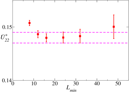
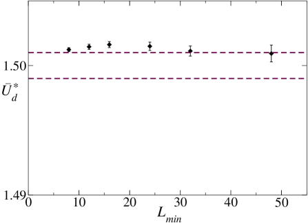
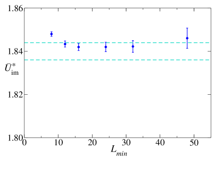
Figure 15: Estimates of $\bar{U}_{22}^{*}$, $\bar{U}_{\rm im}^{*}$, and $\bar{U}_{d}^{*}$ obtained by fitting $\bar{U}_{22}$, $\bar{U}_{\rm im}$, and $\bar{U}_{d}$ for the RBIM at $p=0.55$, to $\bar{U}^{*}+cL^{-\omega_{2}}$ with $\omega_{2}=0.82$. The dashed lines correspond to the estimates of $\bar{U}^{*}$ obtained from the analyses of the data of the RSIM at $p=0.8$.

In this section we analyze the MC data of the RBIM at $p=0.55$ and $p=0.7$ at fixed $R_{\xi}=0.5943$. They are reported in Tables 4 and 5, respectively. We show that their critical behavior is fully consistent with that obtained for the RSIM in Secs. 5 and 6.

7.1 Phenomenological couplings

We first discuss the FSS behavior of the quartic cumulants. In Fig. 6 we have already shown the MC results $\bar{U}_{22}(L)$ for the RBIM at $p=0.55$ and $p=0.7$ versus $L^{-\omega}$ with $\omega=0.33$. Their large-$L$ behavior is perfectly consistent with that observed in the RSIM, all data converging to $\bar{U}_{22}^{*}=0.148(1)$ as $L$ increases. A more quantitative check can be performed by fitting the MC results for $\bar{U}_{\rm im}$. Indeed, as discussed in Sec. 5.6, the leading scaling corrections in $\bar{U}_{\rm im}$ are at least a factor of 10 and a factor of 20 smaller that those in $\bar{U}_{22}$ and $\bar{U}_{d}$, respectively. Thus, for any generic $p$, we should be able to obtain estimates of $\bar{U}_{\rm im}^{*}$ that are more precise than those of $\bar{U}_{22}^{*}$ and $\bar{U}_{d}^{*}$. In particular, we expect errors comparable to that of the RSIM result $\bar{U}_{\rm im}^{*}=1.840(4)$. We fit $\bar{U}_{\rm im}$ to $\bar{U}_{\rm im}^{*}+cL^{-\epsilon}$ with $\epsilon=0.66$ and 0.82 (we remind the reader that the leading scaling corrections to $\bar{U}_{\rm im}$ are proportional to $L^{-2\omega}$ and $L^{-\omega_{2}})$. Results are reported in Fig. 9. They are fully compatible with those obtained in the RSIM at $p=0.8$, confirming that the RBIM belongs to the same universality class of the RSIM.

A direct analysis of $\bar{U}_{22}$ and $\bar{U}_{d}$ for the RBIM at $p=0.7$ gives results with large errors (see the corresponding analysis for the RSIM at $p=0.65$ reported in Sec. 5.3). Universality is verified, though with limited precision. More precise results are obtained for the RBIM at $p=0.55$, since for this value of $p$ the RBIM turns out to be approximately improved. To determine $p^{*}$ for the RBIM we follow the same strategy employed in Sec. 5.4. We determine the correction-to-scaling amplitude $c_{22,11}$ obtaining $c_{22,11}(p=0.55)=-0.01(2)$ and $c_{22,11}(p=0.7)=-0.17(2)$. Then, we assume that for $p\approx 0.55$, $c_{11}(p)\approx a(p-p^{*})$, so that

$$p^{*}=0.55-{1\over a}c_{22,11}(p=0.55).$$ (71)

The constant $a$—only a rough estimate is needed—is again determined as

$$a=\left.{dc_{22,11}\over dp}\right|_{p=p^{*}}\approx{c_{22,11}(p=0.7)-c_{22,11}(p=0.55)\over 0.7-0.55}=-1.07(15).$$ (72)

This gives

$$p^{*}=0.54(2)$$ (73)

for the RBIM. Again, in setting the error we have not considered the error on the linear interpolation (72).

Since the RBIM at $p=0.55$ is approximately improved, we can fit $\bar{U}_{22}$, $\bar{U}_{\rm im}$, and $\bar{U}_{d}$ to $\bar{U}^{*}+cL^{-\omega_{2}}$. In Fig. 15 we show the results for $\omega_{2}=0.82$. They are very stable and in perfect agreement with the results obtained from the FSS analysis of the RSIM at $p=0.8$. Indeed, we obtain

$$\bar{U}_{\rm im}^{*}=1.842(4),\quad\bar{U}_{22}^{*}=0.148(1),\quad\bar{U}_{d}^{*}=1.501(2),$$ (74)

where the error takes into account the uncertainty on $\omega_{2}$. They must be compared with the estimates obtained from the FSS analysis of the RSIM: $\bar{U}_{\rm im}^{*}=1.840(4)$, $\bar{U}_{22}^{*}=0.148(1)$, and $\bar{U}_{d}^{*}=1.500(1)$. These results provide strong evidence for universality between the RSIM and the RBIM.

7.2 Critical temperatures

Let us now estimate $\beta_{c}$ from the estimates of $\beta_{f}$. For $p=0.55$, since the model is approximately improved, we can fit the data of $\beta_{f}$ to $\beta_{c}+cL^{-1/\nu-\omega_{2}}$. We obtain $\beta_{c}=0.4322895(15)$, which is compatible with the MC results of Ref. [21], $\beta_{c}=0.43225(10)$. The analysis of the 19th-order high-temperature expansion of $\chi$ reported in Ref. [8] gave the estimate $\beta_{c}=0.43253(12)$.

For $p=0.7$ we must take into account the leading scaling corrections, i.e. fit $\beta_{f}$ to $\beta_{c}+cL^{-\epsilon}$, where $\epsilon\in[\omega+1/\nu,\omega_{2}+1/\nu]$. We obtain $\beta_{c}=0.326707(2)$, which agrees with the MC estimate $\beta_{c}=0.32670(5)$ of Ref. [21].

7.3 Critical exponents

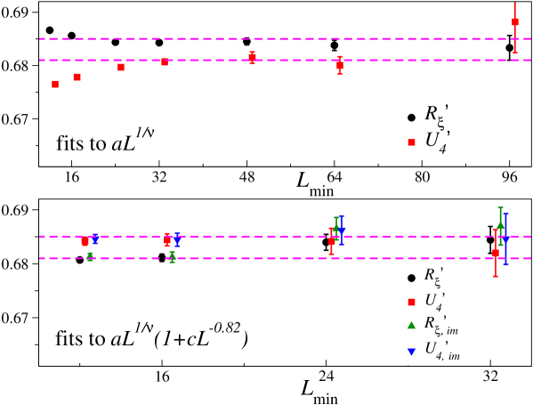
Figure 16: Estimates of the critical exponent $\nu$, obtained by fitting the data of the RBIM at $p=0.55$ (some results are slightly shifted along the $x$-axis to make them visible). The dashed lines correspond to the estimate $\nu=0.683(2)$ obtained in the RSIM at $p=0.8$.

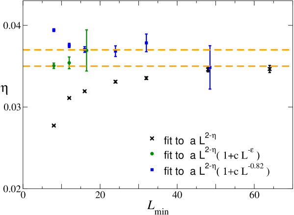
Figure 17: Estimates of the critical exponent $\eta$, obtained by fitting the data of the RBIM at $p=0.55$. The dashes line correspond to the estimate $\eta=0.036(1)$ obtained in the RSIM at $p=0.8$.

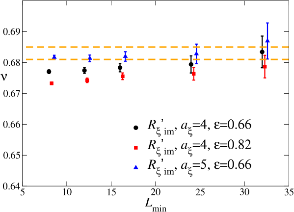
Figure 18: Results for the critical exponent $\nu$, obtained by fitting the data of the RBIM at $p=0.7$ (some results are slightly shifted along the $x$-axis to make them visible). The dashed lines correspond to the estimate $\nu=0.683(2)$ obtained in the RSIM at $p=0.8$.

Let us now consider the critical exponents. Since the RBIM at $p=0.55$ is approximately improved, we perform the same analysis as done for the RSIM at $p=0.8$, see Sec. 5.7. In Fig. 16 we show the results of several fits of the data of the derivative of the phenomenological couplings at $p=0.55$. The estimates obtained by using $R^{\prime}_{\xi}$ and $R^{\prime}_{\xi,{\rm im}}$ are substantially equivalent, as expected because the RBIM at $p=0.55$ is approximately improved. The estimates of $\nu$ shown in Fig. 16 are fully consistent with the estimate $\nu=0.683(2)$ obtained from the FSS analysis of the RSIM at $p=0.8$. Similar conclusions hold for the critical exponent $\eta$. In Fig. 17 we show the results of several fits analogous to those discussed in Sec. 5.9. Again universality is well satisfied: the estimates of $\eta$ are compatible with the RSIM result $\eta=0.036(1)$.

In the case of the RBIM at $p=0.7$, analyses of unimproved quantities give estimates of $\nu$ with large errors. We therefore only consider the improved quantities. In Fig. 18 we show the results of fits of $R^{\prime}_{\xi,{\rm im}}$ for the RBIM at $p=0.7$. They are again substantially consistent with the estimate $\nu=0.683(2)$ obtained from the FSS analysis of the RSIM at $p=0.8$. The MC estimates of $U^{\prime}_{4,{\rm im}}$ are less precise, but again consistent with universality.

Appendix A Field-theory estimate of $\omega_{2}$

In this appendix we estimate $\omega_{2}$ by a reanalysis of its FT six-loop expansion in the massive zero-momentum scheme. In Ref. [11] we performed a direct analysis of the stability matrix at the RDIs fixed point (FP), obtaining $\omega_{2}=0.8(2)$. Here we shall use the method discussed in Ref. [19]—it consists in an expansion around the unstable Ising FP—which allows us to estimate accurately the difference $\omega_{2}-\omega_{\rm Is}$, where $\omega_{\rm Is}$ is the leading correction-to-scaling exponent in the standard Ising model. Since $\omega_{\rm Is}$ is known quite precisely, this method allows us to obtain a precise result for $\omega_{2}$.

In the FT approach one starts from Hamiltonian (4), determining perturbative expansions in powers of the renormalized couplings $u$ and $v$. We normalize them so that $u\approx u_{0}$ and $v\approx v_{0}$ at tree level (these are the normalizations used in Ref. [19]; they differ from those of Ref. [11]). As discussed in Ref. [9], it is more convenient to introduce new variables $y\equiv u+v$ and $z\equiv-u$. The Ising FP is located at $z_{I}^{*}=0$ and $y_{I}^{*}=g_{\rm Is}^{*}$, where [10] $g_{\rm Is}^{*}=23.56(2)$. The RDIs FP is located at $y^{*}=24.7(2)$ and $z^{*}=18.6(3)$ (we use the MC results of Ref. [19] since the FT estimates $y^{*}=24.8(6)$ and $z^{*}=14(2)$ are less precise).

The expansion around the Ising FP can be performed along the Ising-to-RDIs RG trajectory [9], which is obtained as the limit $z_{0}\rightarrow 0^{+}$ ($u_{0}\rightarrow 0^{-}$) of the RG trajectories in the $z$, $y$ plane, see Fig. 1. An effective parametrization of the curve is given by the first few terms of its expansion around $z=0$, which is given by

$$y-y_{I}=T(z)=c_{2}z^{2}+c_{3}z^{3}+\cdots$$ (75)

where [9] $c_{2}=0.0033(1)$ and $c_{3}=1(2)\times 10^{-5}$. The fact that $y-y_{I}$ is of order $z^{2}$ is the main reason why the variable $y$ was introduced and is due to the identity [9]

$$\left.{\partial\beta_{v}\over\partial u}\right|_{u=0}+\left.{\partial\beta_{u}\over\partial u}\right|_{u=0}-\left.{\partial\beta_{v}\over\partial v}\right|_{u=0}=0,$$ (76)

which corresponds to

$$\left.{\partial\beta_{y}\over\partial z}\right|_{z=0}=0.$$ (77)

Performing the variable change $y=g+T(z)$ in the double expansion of a generic quantity $f(y,z)$ in powers of $y$ and $z$, we obtain

$$\bar{f}(g,z)=f(g+T({z}),{z})=\sum_{i}e_{i}(g){z}^{i}.$$ (78)

The coefficients $e_{i}$ must be evaluated at $g=g_{\rm Is}^{*}$. This is done by resumming their perturbative expansions as discussed in Ref. [30]: in particular, we exploit Borel summability and the knowledge of the large-order behavior at the Ising FP.

In Ref. [19] this approach was applied to the standard critical exponents. Here we extend these calculations to the next-to-leading scaling-correction exponent $\omega_{2}$. For this purpose, we consider the stability matrix

$$\Omega=(\partial\beta_{y}/\partial y,\partial\beta_{y}/\partial z;\partial\beta_{z}/\partial y,\partial\beta_{z}/\partial z).$$ (79)

Each entry has an expansion of the form (78), with coefficients $e_{i}(g)$ that are resummed as discussed before. Then, the matrix $\Omega$ is diagonalized, obtaining the expansion of its eigenvalues in powers of $z$ up to $O(z^{3})$. The corresponding coefficients for the smallest eigenvalue are quite large, so that this method does not provide an estimate of $\omega$ which is more precise than that obtained in Ref. [11], i.e. $\omega=0.25(10)$. On the other hand, the expansion coefficients for $\omega_{2}$ are quite small. To order $z^{3}$ we obtain

$$\omega_{2}-\omega_{\rm Is}=\sum_{i}c_{i}z^{i},$$ (80)

$$c_{1}=0,\quad c_{2}=5(2)\times 10^{-5},\quad c_{3}=-2(6)\times 10^{-6},$$ (81)

where $c_{1}=0$ exactly [this is a consequence of relation (77)], and the errors on the coefficients $c_{2}$ and $c_{3}$ are due to the resummation of the corresponding series evaluated at $g_{\rm Is}^{*}$. Expansion (80) is evaluated at $z=18.6(2)$, obtaining

$$\omega_{2}-\omega_{\rm Is}=0.00(5),$$ (82)

where the error takes into account all possible sources of uncertainties: the error on the coefficients, the truncation of the series in powers of $z$, and the uncertainty on the coordinates of the RDIs FP. Then, using the estimate $\omega_{\rm Is}=0.82(3)$, which takes into account the results of Refs. [16, 28, 39] obtained by various approaches, we arrive at the estimate

$$\omega_{2}=0.82(8),$$ (83)

which improves the result $\omega_{2}=0.8(2)$ obtained in Refs. [11, 9].

Appendix B Bias corrections

In this section we discuss the problem of the bias correction needed in the calculations of disorder averages of combinations of thermal averages. As already emphasized in Ref. [38], this is a crucial step in high-precision MC studies of random systems.

To discuss it in full generality, let us indicate with $S$ the state space corresponding to the variables $\sigma$ and with $R$ that corresponding to the dilution variables. Then, we consider a probability function $\pi(\sigma;\rho)$ on $S$ depending parametrically on $\rho$ ($\pi=e^{-\beta{\cal H}}/Z$ in the specific calculation) and a probability $p(\rho)$ on $R$. Averages over $\pi(\sigma;\rho)$ are indicated as $\langle\cdot\rangle$, or with $\langle\cdot\rangle_{\rho}$ when we wish to specify the value $\rho$ used in the calculation. Moreover, we assume $R$ to have a finite number $K$ of elements ($K=2^{V}$ and $K=2^{dV}$ in the RSIM and in the RBIM, respectively). We wish to compute averages of functions $A(\sigma,\rho)$. We first discuss the calculation of

$${\cal O}_{n}\equiv\overline{\langle A\rangle^{n}}=\sum_{\rho}p(\rho)\left[\sum_{\sigma}\pi(\sigma;\rho)A(\sigma,\rho)\right]^{n}.$$ (84)

A numerical strategy to compute ${\cal O}_{n}$ could be the following. Extract $N_{s}$ independent disorder configurations $\rho_{\alpha}$, $\alpha=1,\ldots,N_{s}$, with probability $p(\rho)$ and then, for each $\rho_{\alpha}$, extract $N_{m}$ independent configurations $\sigma_{a,\alpha}$, $a=1,\ldots,N_{m}$, with probability $\pi(\sigma;\rho_{\alpha})$. Then, define the sample average

$$[A]_{\rho_{\alpha}}\equiv{1\over N_{m}}\sum_{a=1}^{N_{m}}A(\sigma_{a,\alpha},\rho_{\alpha}).$$ (85)

A possible estimator of ${\cal O}_{n}$ could be

$${\cal O}_{n}^{\rm est}\equiv{1\over N_{s}}\sum_{\alpha=1}^{N_{s}}[A]_{\rho_{\alpha}}^{n}.$$ (86)

The question is whether ${\cal O}_{n}^{\rm est}$ converges to ${\cal O}_{n}$ defined in Eq. (84) as $N_{s}\to\infty$ at fixed $N_{m}$.

To answer this question, let $N(\rho)$ be the number of $\rho_{\alpha}$ such that $\rho_{\alpha}=\rho$. Eq. (86) can thus be rewritten as

$${\cal O}_{n}^{\rm est}={1\over N_{s}}\sum_{\rho\in R}\sum_{\alpha=1}^{N(\rho)}[A]_{\rho,\alpha}^{n},$$ (87)

where the second sum extends over the $N(\rho)$ terms that appear in Eq. (86) such that $\rho_{\alpha}=\rho$, i.e., which correspond to the same disorder configuration. As $N_{s}\to\infty$, $N(\rho)$ converges to $N_{s}p(\rho)$ with probability 1; thus, as $N_{s}\to\infty$

$$\sum_{\alpha=1}^{N(\rho)}[A]_{\rho,\alpha}^{n}\to N_{s}p(\rho)\times{1\over N(\rho)}\sum_{\alpha=1}^{N(\rho)}[A]_{\rho,\alpha}^{n}\to N_{s}p(\rho)\left\langle[A]_{\rho}^{n}\right\rangle_{\rho}.$$ (88)

Thus, for $N_{s}\to\infty$ we have

$${\cal O}_{n}^{\rm est}=\sum_{\rho}p(\rho)\left\langle[A]_{\rho}^{n}\right\rangle_{\rho}=\overline{\left\langle[A]^{n}\right\rangle}.$$ (89)

Eq. (89) relies only on the limit $N_{s}\to\infty$ and is valid for any $N_{m}$. If $n=1$ we obtain

$$\left\langle[A]\right\rangle_{\rho}={1\over N_{m}}\left\langle\sum_{a=1}^{N_{m}}A(\sigma_{a},\rho)\right\rangle_{\rho}=\left\langle A\right\rangle_{\rho},$$ (90)

so that ${\cal O}_{1}^{\rm est}$ converges to ${\cal O}_{1}$ irrespective of $N_{m}$: one could even take $N_{m}=1$.

This result could have been guessed directly from Eq. (84), since

$${\cal O}_{1}=\sum_{\rho}p(\rho)\pi(\sigma;\rho)A(\sigma,\rho).$$ (91)

A correct sampling is obtained by determining each time a new $\sigma$ and $\rho$ with combined probability $p(\rho)\pi(\sigma;\rho)$. Let us now consider $n=2$. We have

$$\left\langle[A]^{2}\right\rangle_{\rho} = {1\over N_{m}^{2}}\left\langle\sum_{a=1}^{N_{m}}\sum_{b=1}^{N_{m}}A(\sigma_{a},\rho)A(\sigma_{b},\rho)\right\rangle_{\rho}$$ (92)

$$= {1\over N_{m}^{2}}\left[N_{m}(N_{m}-1)\left\langle A\right\rangle_{\rho}^{2}+N_{m}\left\langle A^{2}\right\rangle_{\rho}\right]$$

$$= \left\langle A\right\rangle_{\rho}^{2}+{1\over N_{m}}\left(\left\langle A^{2}\right\rangle_{\rho}-\left\langle A\right\rangle_{\rho}^{2}\right).$$

Thus, we obtain for $N_{s}\to\infty$ at fixed $N_{m}$

$${\cal O}_{2}^{\rm est}\to{\cal O}_{2}+{1\over N_{m}}\left(\overline{\left\langle A^{2}\right\rangle}-\overline{\left\langle A\right\rangle^{2}}\right).$$ (93)

The second term is what is called the bias. Since in the simulations $N_{m}$ is finite and not too large, this term may give rise to systematic deviations larger than statistical errors. It is therefore important to correct the estimator in such a way to eliminate the bias.

For this purpose we divide the $N_{m}$ configurations in $n$ bunches and define the sample average over bunch $i$ of length $N_{m}/n$:

$$[A]_{1/n,i,\rho_{\alpha}}\equiv{n\over N_{m}}\sum_{a=1+(i-1)N_{m}/n}^{iN_{m}/n}A(\sigma_{a,\alpha},\rho_{\alpha}).$$ (94)

A new estimator of ${\cal O}_{n}$ is

$${\cal O}_{n}^{\rm unbiased}\equiv{1\over N_{s}}\sum_{\alpha=1}^{N_{s}}[A]_{1/n,1,\rho_{\alpha}}[A]_{1/n,2,\rho_{\alpha}}\cdots[A]_{1/n,n,\rho_{\alpha}}.$$ (95)

Let us verify that this estimator is unbiased. By repeating the arguments presented above, for $N_{s}\to\infty$ the estimator ${\cal O}_{n}^{\rm unbiased}$ converges to

$${\cal O}_{n}^{\rm unbiased}\to\overline{\left\langle[A]_{1/n,1}[A]_{1/n,2}\cdots[A]_{1/n,n}\right\rangle}.$$ (96)

Because the configurations are assumed to be independent, we have

$$\left\langle[A]_{1/n,1}[A]_{1/n,2}\cdots[A]_{1/n,n}\right\rangle=\left\langle[A]_{1/n,1}\right\rangle\left\langle[A]_{1/n,2}\right\rangle\cdots\left\langle[A]_{1/n,n}\right\rangle=\left\langle A\right\rangle^{n}.$$ (97)

Thus, for any $n$, irrespective of $N_{m}$ (one could even take $N_{m}=n$), ${\cal O}_{n}^{\rm unbiased}$ converges to ${\cal O}_{n}$ as $N_{s}\to\infty$.

The considerations reported above can be trivially extended to disorder averages of products of sample averages. Thus, in order to compute $\overline{\langle A\rangle\langle B\rangle}$, we use

$${1\over 2N_{s}}\sum_{\alpha=1}^{N_{s}}\left([A]_{1/2,1,\rho_{\alpha}}[B]_{1/2,2,\rho_{\alpha}}+[B]_{1/2,1,\rho_{\alpha}}[A]_{1/2,2,\rho_{\alpha}}\right),$$ (98)

while for $\overline{\langle A\rangle\langle B\rangle\langle C\rangle}$ we use

$${1\over 3!N_{s}}\sum_{\alpha=1}^{N_{s}}\left\{[A]_{1/3,1,\rho_{\alpha}}[B]_{1/3,2,\rho_{\alpha}}[C]_{1/3,3,\rho_{\alpha}}+\hbox{5 permutations}\right\}.$$ (99)

In the case of $n$ terms, we divide the $N_{m}$ estimates into $n$ parts and then consider all the $n!$ permutations.

In this paper we extensively use the reweighting technique that requires the computation of averages of the form

$$R_{A,B}\equiv\overline{\left({\langle A\rangle\over\langle B\rangle}\right)},$$ (100)

where the disorder average should be done after computing the ratio. Indeed, given a MC run at inverse temperature $\beta$ the mean value of an observable $\cal O$ at $\beta+\Delta\beta$ is given by

$$\langle{\cal O}\rangle_{\beta+\Delta\beta}=\langle{\cal O}e^{-\Delta\beta{\cal H}}\rangle_{\beta}/\langle e^{-\Delta\beta{\cal H}}\rangle_{\beta}.$$ (101)

To compute $R_{A,B}$ we consider an estimator of the form

$$R_{A,B}^{\rm est}\equiv{1\over 2N_{s}}\sum_{\alpha=1}^{N_{s}}\left([A]_{1/2,1,\rho_{\alpha}}\left\{{1\over B}\right\}_{1/2,2,\rho_{\alpha}}+[A]_{1/2,2,\rho_{\alpha}}\left\{{1\over B}\right\}_{1/2,1,\rho_{\alpha}}\right),$$ (102)

where $\{\cdot\}$ should be defined so that

$$\left\{{1\over B}\right\}\to{1\over\langle B\rangle}$$ (103)

for $N_{s}\to\infty$ and any $N_{m}$ (the suffix $1/2,i$ has the same meaning as before). We have not been able to define an estimator with this property. We thus use a biased estimator, with a bias of order $N_{m}^{-2}$. Consider

$$\left\langle{1\over[B]_{\rho}}\right\rangle_{\rho}={1\over\langle B\rangle_{\rho}}\left\langle\left[1+{1\over N_{m}}\sum_{a}\left({B(\sigma_{a},\rho)-\langle B\rangle_{\rho}\over\langle B\rangle_{\rho}}\right)\right]^{-1}\right\rangle_{\rho}.$$ (104)

Assuming $N_{m}$ large, we can expand the term in brackets, keeping the first nonvanishing term:

$$\left\langle{1\over[B]_{\rho}}\right\rangle_{\rho}={1\over\langle B\rangle_{\rho}}\left\langle\left[1+{1\over N_{m}^{2}}\sum_{ab}\left({B(\sigma_{a},\rho)-\langle B\rangle_{\rho}\over\langle B\rangle_{\rho}}\right)\left({B(\sigma_{b},\rho)-\langle B\rangle_{\rho}\over\langle B\rangle_{\rho}}\right)\right]\right\rangle_{\rho}+\cdots$$

$$={1\over\langle B\rangle_{\rho}}\left(1+{1\over N_{m}}{\langle B^{2}\rangle_{\rho}-\langle B\rangle_{\rho}^{2}\over\langle B\rangle_{\rho}^{2}}+O(N_{m}^{-2})\right).$$ (105)

Thus, if we define

$$\left\{{1\over B}\right\}={1\over[B]}\left(1-{1\over N_{m}}{[B^{2}]-[B]^{2}\over[B]^{2}}\right),$$ (106)

which is such that

$$\left<\left\{{1\over B}\right\}\right\rangle={1\over\langle B\rangle}(1+O(N_{m}^{-2})),$$ (107)

the estimator (102) converges to $R_{AB}$ with corrections of order $N_{m}^{-2}$. Thus, when using the reweighting technique, $N_{m}$ is crucial and cannot be too small.

In this paper we also compute derivatives of different observables with respect to $\beta$. They can be related to connected correlation function as

$$\frac{\partial\overline{\langle{\cal O}\rangle}}{\partial\beta}=-\overline{\langle{\cal O}{\cal H}\rangle-\langle O\rangle\langle{\cal H}\rangle}.$$ (108)

Therefore, if we apply the reweighting technique, we need to compute terms of the form

$$R_{AB,C}\equiv\overline{\langle A\rangle\langle B\rangle\over\langle C\rangle^{2}},$$ (109)

with $A={\cal O}e^{-\Delta\beta{\cal H}}$, $B={\cal H}e^{-\Delta\beta{\cal H}}$, and $C=e^{-\Delta\beta{\cal H}}$. A possible estimator (this is the one that is used in the paper) is

$${1\over 4!N_{s}}\sum_{\alpha=1}^{N_{s}}\left[[A]_{1/4,1,\rho_{\alpha}}[B]_{1/4,2,\rho_{\alpha}}\left\{{1\over C}\right\}_{1/4,3,\rho_{\alpha}}\left\{{1\over C}\right\}_{1/4,4,\rho_{\alpha}}+\hbox{permutations}\right].$$ (110)

The formulae we have derived above rely on two assumptions: (i) different configurations obtained with the same disorder $\rho_{\alpha}$ are uncorrelated; (ii) configurations $\sigma$ are extracted with probability $\pi(\sigma,\rho)$. None of these two hypothesis is exactly verified in practical calculations. Hypothesis (i) is violated because MC simulations usually provide correlated sequences of configurations. Correlations change some of the conclusions presented above. First, the estimator (95) is no longer unbiased, except in the case $n=1$. To explain this point, let us consider the specific case $n=2$. In the presence of correlations

$$\left\langle A(\sigma_{a\alpha},\rho_{\alpha})A(\sigma_{b\alpha},\rho_{\alpha})\right\rangle_{\rho_{\alpha}}=\langle A\rangle_{\rho_{\alpha}}^{2}+(\hbox{var}_{\rho_{\alpha}}A)C(|a-b|),$$ (111)

where $\hbox{var}\,A=\langle A\rangle^{2}-\langle A\rangle^{2}$ and $C(t)$ is the autocorrelation function. Then

$$\left\langle[A]_{1/2,1,\rho_{\alpha}}[A]_{1/2,2,\rho_{\alpha}}\right\rangle_{\rho_{\alpha}}$$

$$=\langle A\rangle_{\rho_{\alpha}}^{2}+{4\hbox{var}_{\rho_{\alpha}}A\over N_{m}^{2}}\left[\sum_{a=1}^{N_{m}/2}aC(a)+\sum_{a=N_{m}/2+1}^{N_{m}-1}(N_{m}-a)C(a)\right].$$ (112)

If $C(t)$ decays fast enough the term in brackets is finite for $N_{m}\to\infty$. If we further assume $C(t)=\exp(-t/\tau)$, we find that the bias is of order $(\tau/N_{m})^{2}$. Thus, for $n\geq 2$ the estimator (95) is biased. Therefore, it is no longer possible to take $N_{m}$ at will. To avoid the bias, $N_{m}$ should be significantly larger than the autocorrelation time. Analogously, Eq. (106) is correct only in the absence of correlations. Otherwise one should define

$$\left\{{1\over B}\right\}={1\over[B]}\left(1-{2\tau_{B,{\rm int}}\over N_{m}}{[B^{2}]-[B]^{2}\over[B]^{2}}\right),$$ (113)

where $\tau_{B,{\rm int}}$ is the integrated autocorrelation time associated with $B$. In the present work the MC algorithm is very efficient, so that our measurements should be nearly independent. Thus, we have always used Eq. (106).

The second assumption that we have made is that configurations $\sigma_{a,\alpha}$ are extracted with probability $\pi(\sigma,\rho_{\alpha})$. In MC calculations this is never the case: configurations are obtained by using a Markov chain that starts from a nonequilibrium configuration. Therefore $\sigma_{a,\alpha}$ are generated by using a distribution that converges to $\pi(\sigma,\rho_{\alpha})$ only asymptotically. This is the so-called inizialization bias. This bias, which is of order $N_{m}^{-1}$, cannot be avoided. However, by discarding a sufficiently large number of initial configurations one can reduce it arbitrarily. Note that, as $N_{s}$ is increased, either $N_{m}$ or the number of discarded configurations should be increased too.

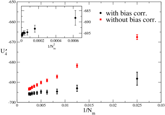
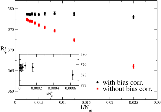
Figure 19: $U^{\prime}_{4}$ and $R^{\prime}_{\xi}$ for a run of the RSIM model at $L=64$, $p=0.8$, $N_{s}=60000$, $\beta_{\rm run}=0.285742$, reweighted at $R_{\xi}$ = 0.5943 as a function of $1/N_{m}$. In the insets we show the results for the bias-corrected estimates versus $1/N_{m}^{2}$. We report data with $N_{m}=40,80,120,\ldots,400$.

Of course, the practically interesting question is whether, with the values of $N_{m}$ and $N_{s}$ used in the MC simulations, bias corrections are relevant or not. For this purpose, in Fig. 19 we compare, for a specific run of the RSIM at $p=0.8$, the value of the derivatives $U^{\prime}_{4}$, $R^{\prime}_{\xi}$, with and without bias correction, as a function of $N_{m}$; data obtained for $\beta=0.2857420$ are reweighted to have $R_{\xi}=0.5943$ [this corresponds to $\beta_{f}=0.2857478(18)$]. The average without bias correction has been estimated by using

$${1\over N_{s}}\sum_{\alpha=1}^{N_{s}}{[A]_{\rho_{\alpha}}[B]_{\rho_{\alpha}}\over[C]^{2}_{\rho_{\alpha}}}$$ (114)

while the bias-corrected estimate corresponds to Eq. (110). From the figure, we see that the biased estimate shows a systematic drift, which, as expected, is linear in $1/N_{m}$. The bias-corrected estimate is instead essentially flat; deviations are observed only for $U_{4}^{\prime}$ for $N_{m}\mathrel{\hbox to0.0pt{\lower 3.0pt\hbox{$\mathchar 536\relax$}\hss}\raise 2.0pt\hbox{$\mathchar 316\relax$}}100$. As expected, they apparently decrease as $1/N_{m}^{2}$. Note, that even for $N_{m}=400$ the biased estimate differs within error bars from the bias-corrected one. Thus, with the precision of our calculations, the bias correction is essential for both $R_{\xi}^{\prime}$ and $U_{4}^{\prime}$.

We would like to point out that the expressions obtained here are somewhat different from those proposed in Ref. [38]. Only for $\overline{\langle A\rangle\langle B\rangle}$ are they identical. We report here the expressions for $R_{AB}$ and $R_{AB,C}$:

$$R_{A,B}^{\rm est} = {2\over N_{s}}\sum_{\alpha=1}^{N_{s}}\left[{[A]\over[B]}-{[A]_{1/2,1}\over 4[B]_{1/2,1}}-{[A]_{1/2,2}\over 4[B]_{1/2,2}}\right],$$

$$R_{AB,C}^{\rm est} = {2\over N_{s}}\sum_{\alpha=1}^{N_{s}}\left[{[A][B]\over[C]^{2}}-{[A]_{1/2,1}[B]_{1/2,1}\over 4[C]_{1/2,1}^{2}}-{[A]_{1/2,2}[B]_{1/2,2}\over 4[C]_{1/2,2}^{2}}\right].$$ (115)

The idea behind these formulas is the following. Consider ${\cal O}$ which is an arbitrary function of thermal averages. To compute $\overline{\cal O}$, consider an arbitrary estimator ${\cal O}^{\rm est}$ of $\overline{\cal O}$. For $N_{s}\to\infty$ at fixed $N_{m}$, ${\cal O}^{\rm est}$ converges to

$$\overline{\cal O}+{a\over N_{m}}+O(1/N_{m}^{2}).$$ (116)

A better estimator, without the $1/N_{m}$ correction, is obtained by considering

$${\cal O}^{\rm est,unb}=2{\cal O}^{\rm est}-{1\over 2}{\cal O}^{\rm est}_{1/2,1}-{1\over 2}{\cal O}^{\rm est}_{1/2,2}.$$ (117)

Here ${\cal O}^{\rm est}$ is determined by using all $N_{m}$ measures, while ${\cal O}^{\rm est}_{1/2,1}$ and ${\cal O}^{\rm est}_{1/2,2}$ are computed by using the first half and the second half of the measures, respectively. It is easy to see, by substituting the behavior (116) in Eq. (117), that the new estimator has no corrections of order $1/N_{m}$.

References

References

- [1] Belanger D P, Experimental Characterization of the Ising Model in Disordered Antiferromagnets, 2000, Braz. J. Phys. 30 682 [cond-mat/0009029].
- [2] Fishman S and Aharony A, Random field effects in disordered anisotropic antiferromagnets, 1979, J. Phys. C: Solid State Phys.12 L729 Cardy J L, Random-field effects in site-disordered Ising antiferromagnets, 1984, Phys. Rev.B 29 505
- [3] Calabrese P, Pelissetto A and Vicari E, Crossover from random-exchange to random-field critical behavior in Ising systems, 2003, Phys. Rev.B 68 092409 [cond-mat/0305041]
- [4] Aharony A, in 1976 Phase Transitions and Critical Phenomena, vol 6, ed C Domb and M S Green (New York: Academic Press) p 357
- [5] Stinchcombe R B, in 1983 Phase Transitions and Critical Phenomena, vol 7, ed C Domb and J L Lebowitz (New York: Academic Press) p 152
- [6] Pelissetto A and Vicari E, Critical phenomena and renormalization-group theory, 2002, Phys. Rept. 368 549 [cond-mat/0012164]
- [7] Folk R, Holovatch Yu and Yavors’kii T, Critical exponents of a three dimensional weakly diluted quenched Ising model, 2003, Uspekhi Fiz. Nauk 173 175 [Phys. Usp. 46 175] [cond-mat/0106468]
- [8] Janke W, Berche B, Chatelain C, Berche P E and Hellmund M, Quenched disordered ferromagnets, 2005, PoS(LAT2005)018
- [9] Calabrese P, Parruccini P, Pelissetto A and Vicari E, Crossover behavior in three-dimensional dilute Ising systems, 2004, Phys. Rev.E 69 036120 [cond-mat/0307699]
- [10] Campostrini M, Pelissetto A, Rossi P and Vicari E, 25th order high-temperature expansion results for three-dimensional Ising-like systems on the simple cubic lattice, 2002, Phys. Rev.E 65 066127 [cond-mat/0201180]
- [11] Pelissetto A and Vicari E, Randomly dilute spin models: a six-loop field-theoretic study, 2000, Phys. Rev.B 62 6393 [cond-mat/0002402]
- [12] Pakhnin D V and Sokolov A I, Five-loop renormalization-group expansions for the three-dimensional n-vector cubic model and critical exponents for impure Ising systems, 2000, Phys. Rev.B 61 15130 [cond-mat/9912071]
- [13] Bray A J, McCarthy T, Moore M A, Reger J D and Young A P, Summability of perturbation expansions in disordered systems: Results for a toy model, 1987, Phys. Rev.B 36 2212
- [14] McKane A J, Structure of the perturbation expansion in a simple quenched system, 1994, Phys. Rev.B 49 12003
- [15] Álvarez G, Martín-Mayor V and Ruiz-Lorenzo J J, Summability of the perturbative expansion for a zero-dimensional disordered spin model, 2000, J. Phys. A: Math. Gen.33 841 [cond-mat/9910186]
- [16] Guida R and Zinn-Justin J, Critical exponents of the N-vector model, 1998, J. Phys. A: Math. Gen.31 8103 [cond-mat/9803240]
- [17] Calabrese P, De Prato M, Pelissetto A and Vicari E, Critical equation of state of randomly diluted Ising systems, 2003, Phys. Rev.B 68 134418 [cond-mat/0305434]
- [18] Ballesteros H G, Fernández L A, Martín-Mayor V, Muñoz Sudupe A, Parisi G and Ruiz-Lorenzo J J, Critical exponents of the three dimensional diluted Ising model, 1998, Phys. Rev.B 58 2740 [cond-mat/9802273]
- [19] Calabrese P, Martín-Mayor V, Pelissetto A and Vicari E, The three-dimensional randomly dilute Ising model: Monte Carlo results, 2003, Phys. Rev.E 68 036136 [cond-mat/0306272]
- [20] Hukushima K, Random fixed point of three-dimensional random-bond Ising ising models, 2000, J. Phys. Soc. Japan 69 631
- [21] Berche P E, Chatelain C, Berche B and Janke W, Bond dilution in the 3D Ising model: a Monte Carlo study, 2004, Eur. Phys. J. B 38 463 [cond-mat/0402596]
- [22] Hellmund M and Janke W, High-temperature series for the bond-diluted Ising model in 3, 4, and 5 dimensions, 2006, cond-mat/0606320
- [23] Wegner F J, in 1976 Phase Transitions and Critical Phenomena, vol 6, ed C Domb and M S Green (New York: Academic Press)
- [24] Aharony A and Fisher M E, Nonlinear scaling fields and corrections to scaling near criticality, 1983, Phys. Rev.B 27, 4394
- [25] Salas J and Sokal A D, Universal amplitude ratios in the critical two-dimensional Ising model on a torus, 2000, J. Stat. Phys. 98 551 [cond-mat/9904038v1]
- [26] Caselle M, Hasenbusch M, Pelissetto A and Vicari E, Irrelevant operators in the two-dimensional Ising model, 2002, J. Phys. A: Math. Gen.35 4861 [cond-mat/0106372]
- [27] Campostrini M, Hasenbusch M, Pelissetto A and Vicari E, Theoretical estimates of the critical exponents of the superfluid transition in 4He by lattice methods, 2006, Phys. Rev.B 74 144506 [cond-mat/0605083]
- [28] Hasenbusch M, A Monte Carlo study of leading order scaling corrections of theory on a three dimensional lattice, 1999, J. Phys. A: Math. Gen.32 4851 [hep-lat/9902026]
- [29] Hasenbusch M, Pelissetto A and Vicari E, Multicritical behavior in the fully frustrated XY model and related systems, 2005, J. Stat. Mech.: Theor and Exp P12002 [cond-mat/0509682]
- [30] Carmona J M, Pelissetto A and Vicari E, The -component Ginzburg-Landau Hamiltonian with cubic symmetry: a six-loop study, 2000, Phys. Rev.B 61, 15136 [cond-mat/9912115]
- [31] Privman V, in 1990 Finite scaling and Numerical Simulations of Statistical Systems, ed V Privman (Singapore: World Scientific)
- [32] Caselle M, Hasenbusch M, Pelissetto A and Vicari E, High-precision estimate of in the 2D Ising model, 2000 J. Phys. A: Math. Gen.33, 8171 [hep-th/0003049]
- [33] Calabrese P, Caselle M, Celi A, Pelissetto A and Vicari E, Non-analyticity of the Callan-Symanzik -function of two-dimensional models, 2000 J. Phys. A: Math. Gen.33, 8155 [hep-th/0005254]
- [34] Caracciolo S and Pelissetto A, Corrections to finite-size scaling in the lattice -vector model for , 1998 Phys. Rev.D 58, 105007 [hep-lat/9804001]
- [35] Campostrini M, Hasenbusch M, Pelissetto A, Rossi P and Vicari E, Critical behavior of the three-dimensional XY universality class, 2001, Phys. Rev.B 63 214503 [cond-mat/0010360]
- [36] Swendsen R H and Wang J-S, Nonuniversal critical dynamics in Monte Carlo simulations, 1987 Phys. Rev. Lett.58 86
- [37] Wolff U, Collective Monte Carlo updating for spin systems, 1989 Phys. Rev. Lett.62 361
- [38] Ballesteros H G, Fernández L A, Martín-Mayor V, Muñoz Sudupe A, Parisi G and Ruiz-Lorenzo J J, The four-dimensional site-diluted Ising model: A finite-size scaling study, 1998, Nucl. Phys. B 512 681 [hep-lat/9707017]
- [39] Deng Y and Blöte H W J, Simultaneous analysis of several models in the three-dimensional Ising universality class, 2003, Phys. Rev.E 68 036125