Spin-1 chain with spin-1/2 excitations in the bulk

Abstract

We present a spin-1 chain with a Hamiltonian which has three exactly solvable ground states. Two of these are fully dimerized, analogous to the Majumdar-Ghosh (MG) states of a spin-1/2 chain, while the third is of the Affleck-Kennedy-Lieb-Tasaki (AKLT) type. We use variational and numerical methods to study the low-energy excitations which interpolate between these ground states in different ways. In particular, there is a spin-1/2 excitation which interpolates between the MG and AKLT ground states; this is the lowest excitation of the system and it has a surprisingly small gap. We discuss generalizations of our model of spin fractionalization to higher spin chains and higher dimensions.

I Introduction

Quantum spin systems in one dimension have been studied extensively for many years. In some seminal papers, Haldane predicted theoretically that integer spin chains with nearest neighbor Heisenberg antiferromagnetic interactions should have a gap between the ground state and the first excited state haldane ; this was then observed experimentally in a spin-1 system buyers ; renard ; ma and confirmed numerically night ; takahashi ; white . Haldane’s analysis used a field theoretic description of the long-distance and low-energy modes of the spin system affleck1 ; fradkin ; auerbach ; sierra . Affleck, Kennedy, Lieb and Tasaki (AKLT) then showed that the ground state of the spin-1 chain can be variationally understood as a state in which each spin-1 is thought of as a symmetric combination of two spin-1/2’s, and the two spin-1/2’s at each site form a singlet with the spin-1/2’s of the neighboring sites aklt . The excitations are given by variational states in which one of these singlets is replaced by a triplet. It was shown later that the AKLT state can be written as a matrix product state klumper .

If a spin chain has sufficiently strong next-nearest-neighbor interactions, the system is frustrated and its low-energy properties can be quite different from those of the unfrustrated system. For instance, the spin-1/2 chain with both nearest neighbor ($J_{1}$) and next-nearest neighbor ($J_{2}$) antiferromagnetic interactions is gapless if $J_{2}=0$, but is gapped if $J_{2}/J_{1}\gtrsim 0.2411$ okamoto ; chitra . In the latter case, the ground state is doubly degenerate as expected by the Lieb-Schultz-Mattis theorem lieb . In particular, for the Majumdar-Ghosh (MG) model given by $J_{2}/J_{1}=1/2$, the ground states are exactly solvable majumdar and consist of products of nearest-neighbor singlet states as will be described below. The lowest excited states then consist of spin-1/2’s interpolating between the two ground states shastry . Hence the excitations of the MG model have spin 1/2 in contrast to the excitations of the AKLT model which have spin 1.

The excitations described above exist in the bulk; they contribute to thermodynamic quantities like the magnetic susceptibility and the specific heat. In addition to these excitations, a gapped chain with a finite number of sites may also have degrees of freedom localized at the edges. For instance, the AKLT model on an open chain has spin-1/2 degrees of freedom at the edges white ; these can be thought of as remnants of the two spin-1/2’s of which each spin-1 is composed. These edge degrees of freedom have been studied using field theoretic methods naveen . It may be interesting to consider spin-1 chains which have spin-1/2 excitations in the bulk, as this would provide an example of spin fractionalization.

Spin fractionalization was first proposed by Faddeev and Takhtajan in the spin-1/2 antiferromagnetic chain faddeev ; the idea is that the elementary excitations, called spinons, carry spin-1/2. This was confirmed experimentally in a one-dimensional spin-1/2 system $KCuF_{3}$ tennant . It was later shown by Anderson and others that spin fractionalization can also occur in higher dimensional systems with resonating valence bond ground states anderson ; wen . This idea has been used to understand the low-lying excitations in a two-dimensional spin-1/2 system $Cs_{2}CuCl_{4}$ coldea ; yunoki . In contrast to these examples of spin fractionalization in spin-1/2 systems, we are proposing a model of spin fractionalization in higher spin systems in this paper.

A spin-1/2 excitation existing in the bulk of a spin-1 chain must clearly have two different ground states on its left and right. For instance, the ground state on the left could be of the MG type in which each spin-1 forms a singlet with one of its neighbors, while the ground state on the right could be of the AKLT type. The spin-1/2 excitation can then be thought of as the edge degree of freedom of the AKLT part of the chain. To realize this kind of an excitation, we require a Hamiltonian for which both MG and AKLT states are ground states. We will present such a Hamiltonian in Sec. II; it contains interactions involving three neighboring sites. We will present a variational estimate of different possible excitations of the model, and will show that the spin-1/2 excitation has the lowest variational energy. In Sec. III, we will present numerical results for finite chains, with both open and periodic boundary conditions. These will confirm that the spin-1/2 excitations indeed have the lowest energy; with periodic boundary conditions, such excitations must occur in pairs. In Sec. IV, we will discuss how our model can be generalized to higher spins and higher dimensions, i.e., how one can construct models which have spin $S$ at each site and spin $S^{\prime}$ excitations in the bulk, with $S^{\prime}<S$. We will make some concluding remarks in Sec. V.

II A spin-1 chain

II.1 Hamiltonian and ground states

We will first present what appears to be the simplest Hamiltonian of an infinite spin-1 chain which has exactly three ground states. This Hamiltonian is motivated by the following arguments. Given three spin-1’s ${\vec{S}}_{1},{\vec{S}}_{2}$ and ${\vec{S}}_{3}$, let us define the projection operators $P_{S}$ which projects on to states with total spin $S$, where $S$ can be 0, 1, 2 or 3. Now consider a three-spin Hamiltonian of the form $h=c_{2}P_{2}+c_{3}P_{3}$, where $c_{2},c_{3}>0$. The ground states of $h$ are all the states whose total spin is equal to 0 or 1; all such states have zero energy. All the excited states have strictly positive energies. If we think of each of the spin-1’s as being a triplet combination of two spin-1/2’s, these ground states correspond to states in which at least four of the six spin-1/2’s form singlets amongst each other. The remaining two spin-1/2’s can at most form a total spin of 1, no matter how they combine with each other. Now, a particular Hamiltonian of the above type is $h=S_{tot}^{2}(S_{tot}^{2}-2)$, where $S_{tot}^{2}=({\vec{S}}_{1}+{\vec{S}}_{2}+{\vec{S}}_{3})^{2}$; this corresponds to the coefficients $c_{2}=24$ and $c_{3}=120$. This is the simplest Hamiltonian with ground state spins being equal to 0 and 1 in the sense that it has the lowest possible powers of the spin operators ${\vec{S}}_{i}$.

We now consider a Hamiltonian for the spin-1 chain of the form

$$H = J~{}\sum_{n}~{}h_{n}~{},$$

$${\rm where}\quad h_{n} = ({\vec{S}}_{n-1}+{\vec{S}}_{n}+{\vec{S}}_{n+1})^{2}$$ (1)

$$\times~{}[({\vec{S}}_{n-1}+{\vec{S}}_{n}+{\vec{S}}_{n+1})^{2}~{}-~{}2]~{}.$$

(We will set the exchange constant $J$ equal to 1). The ground states of this Hamiltonian must have at least two singlet bonds within every group of three neighboring spins. It is then easy to see that there are three degenerate ground states with zero energy of the forms shown in Fig. 1. The analytical expressions for these three states are as follows. Let us define the singlet combination of two spin-1’s at sites $m$ and $n$ as $|S(m,n)\rangle=[|1,-1\rangle_{mn}-|0,0\rangle_{mn}+|-1,1\rangle_{mn}]/\sqrt{3}$, where we have used the $S^{z}$ components to label the states. Then the first two ground states of (1) are given by tensor products of singlets between nearest neighbors of the form

$$|I\rangle = \prod_{n=-\infty}^{\infty}~{}|S(2n,2n+1)\rangle~{},$$

$${\rm and}\quad|II\rangle = \prod_{n=-\infty}^{\infty}~{}|S(2n-1,2n)\rangle~{}.$$ (2)

These are generalizations of the two ground states of the spin-1/2 chain at the MG point majumdar .

Figure 1: The three degenerate ground states. Each solid circle represents a spin $1/2$, and the lines denote singlet bonds.

The third ground state of Eq. (1) is the AKLT state. This can be written as a matrix product state klumper . At a site $n$, let us define the matrix

$$M_{n} = \left(\begin{array}[]{cc}\sqrt{1/3}~{}|0\rangle_{n}&\sqrt{2/3}~{}|-1\rangle_{n}\\ -\sqrt{2/3}~{}|1\rangle_{n}&-\sqrt{1/3}~{}|0\rangle_{n}\end{array}\right)~{}.$$ (5)

Then the AKLT state is given by the matrix product

$$|III\rangle~{}=~{}\prod_{n=-\infty}^{\infty}~{}M_{n}~{}.$$ (6)

The matrix in Eq. (5) is motivated as follows arovas . For a spin-1/2 object, we can use $u=\cos(\theta/2)e^{i\phi/2}$ and $v=\sin(\theta/2)e^{-i\phi/2}$ to describe the spin-up and spin-down states respectively. The spin operators are given by $S^{z}=(u\partial_{u}-v\partial_{v})/2$, $S^{+}=u\partial_{v}$, and $S^{-}=v\partial_{u}$; the total spin is $S=(u\partial_{u}+v\partial_{v})/2$. The inner product in the $(u,v)$ space is defined by the integration measure $d\Omega=\sin\theta d\theta d\phi/(4\pi)$. The correctly normalized spin-1/2 states are given by $|1/2\rangle=\sqrt{2}u$ and $|-1/2\rangle=\sqrt{2}v$. For a spin-1 object, the normalized states are given by $|1\rangle=\sqrt{3}u^{2}$, $|0\rangle=\sqrt{6}uv$, and $|-1\rangle=\sqrt{3}v^{2}$. A singlet formed by spin-1/2’s at sites $n$ and $n+1$ is given by

$$u_{i}v_{i+1}~{}-~{}v_{i}u_{i+1}~{}=~{}\left(\begin{array}[]{cc}u_{i}&v_{i}\end{array}\right)~{}\left(\begin{array}[]{c}v_{i+1}\\ -u_{i+1}\end{array}\right)~{}.$$ (7)

The matrix in Eq. (5) is obtained by combining a column and a row for site $n$ as

$$M_{n}~{}=~{}\sqrt{2}~{}\left(\begin{array}[]{c}v_{n}\\ -u_{n}\end{array}\right)~{}\left(\begin{array}[]{cc}u_{n}&v_{n}\end{array}\right)~{}.$$ (8)

The normalization of $M_{n}$ has been chosen so that the norm of the AKLT state in Eq. (6) is given by

$$Tr\left(\begin{array}[]{cc}1/3&2/3\\ 2/3&1/3\end{array}\right)^{N}~{}=~{}1\quad{\rm in~{}the~{}limit~{}N\to\infty}~{}.$$ (9)

The three states defined in Eqs. (2) and (6) are orthonormal for the infinite chain. We do not have an analytical proof that these are the only ground states of Eq. (1). However, we will provide numerical evidence in Sec. III that there are no other ground states, except for some additional degeneracies in open chains due to degrees of freedom at the edges.

The structure factor in a ground state is given by

$$S(q)~{}=~{}\frac{1}{N}~{}\sum_{m,n}~{}e^{-iq(m-n)}~{}\langle~{}{\vec{S}}_{m}\cdot{\vec{S}}_{n}\rangle~{},$$ (10)

where $N$ is the number of sites in the chain, and we eventually have to take the limit $N\to\infty$. In the three ground states given above, we find that arovas

$$S^{I}(q) = S^{II}(q)~{}=~{}2~{}(1~{}-~{}\cos q)~{},$$

$${\rm and}\quad S^{III}(q) = \frac{6~{}(1~{}-~{}\cos q)}{5~{}+~{}3\cos q}~{}.$$ (11)

II.2 Excited states

We will now study the excited states using a variational technique shastry ; caspers ; sen . Given two ground states $A$ and $B$, which could be any of the states $I$, $II$ or $III$, one can consider a ‘domain wall’ state $|n\rangle$ which interpolates between the two at site $n$. We can then superpose such states to form momentum eigenstates $|k\rangle$ as shown below, and obtain a variational estimate of the energy $E_{var}(k)=\langle k|H|k\rangle/\langle k|k\rangle$. We will now do this for various possible combinations of the two ground states $A$ and $B$ on the left and right. There are four different cases to consider. In each case, we will form an excited state by breaking as few singlet bonds as possible.

Figure 2: Various possible excitations interpolating between different ground states. The lines denote singlet bonds, and each isolated circle denotes a free spin 1/2.

(i) We first consider a state interpolating between ground states $I$ on the left and $II$ on the right as shown in Fig. 2 (i). This is given by

$$|2n(I,II)\rangle = \prod_{m=-\infty}^{n}~{}|S(2m-2,2m-1)\rangle\otimes|1\rangle_{2n}$$ (12)

$$\otimes\prod_{m=n}^{\infty}~{}|S(2m+1,2m+2)\rangle~{}.$$

This is a state with $S_{tot}^{z}=1$. We then find that

$$\langle 2m(I,II)|2n(I,II)\rangle = (1/3)^{|n-m|}~{},$$

$$\langle 2m(I,II)|H|2n(I,II)\rangle = 40~{}\delta_{m,n}~{}.$$ (13)

If we form the momentum eigenstate

$$|k\rangle~{}=~{}\sum_{n}~{}e^{ik2n}~{}|2n\rangle~{},$$ (14)

we find that

$$\langle k|k\rangle = \frac{2N}{5~{}-~{}3\cos(2k)}~{},$$

$${\rm and}\quad\langle k|H|k\rangle = 20N~{}.$$ (15)

From Eq. (15), the variational energy is given by

$$E_{var}(k)~{}=~{}10~{}[5~{}-~{}3\cos(2k)]~{}.$$ (16)

The minimum of this lies at $k=0$, where $E_{var}(0)=20$.

(ii) Next we consider a state interpolating between ground states $I$ on both the left and the right as shown in Fig. 2 (ii). This is obtained by replacing a singlet $|S(2n,2n+1)\rangle$ by a triplet. We thus have

$$|2n(I,I)\rangle = \prod_{m=-\infty}^{n}~{}|S(2m-2,2m-1)\rangle$$ (17)

$$\otimes~{}\frac{1}{\sqrt{2}}~{}[|1,0\rangle_{2n,2n+1}~{}-~{}|0,1\rangle_{2n,2n+1}]$$

$$\otimes\prod_{m=n+1}^{\infty}~{}|S(2m,2m+1)\rangle~{}.$$

This is a state with $S_{tot}^{z}=1$. We find that

$$\langle 2m(I,I)|2n(I,I)\rangle = \delta_{m,n}~{},$$

$$\langle 2m(I,I)|H|2n(I,I)\rangle = \frac{80}{3}~{}\delta_{m,n}~{}.$$ (18)

A momentum eigenstate defined as in Eq. (14) satisfies

$$\langle k|k\rangle~{}=~{}\frac{N}{2}~{},\quad{\rm and}\quad\langle k|H|k\rangle~{}=~{}\frac{40N}{3}~{}.$$ (19)

Hence the variational energy is

$$E_{var}(k)~{}=~{}80/3~{}\simeq~{}26.67$$ (20)

independent of the value of $k$.

(iii) We now consider a state interpolating between ground states $III$ on the left and $I$ on the right as shown in Fig. 2 (iii). The ground state $III$ must end with one singlet bond between the spin-1/2’s at site $2n$ and $2n+1$, along with a free spin 1/2 at site $2n+1$. We therefore take a state which is of the AKLT type from $-\infty$ to site $2n$; this is followed by a column multiplied by a free spin 1/2 at the site $2n+1$ of the form

$$\sqrt{2}~{}\left(\begin{array}[]{c}v_{2n+1}\\ -u_{2n+1}\end{array}\right)~{}u_{2n+1}~{}=~{}\left(\begin{array}[]{c}\sqrt{1/3}~{}|0\rangle_{2n+1}\\ -\sqrt{2/3}~{}|1\rangle_{2n+1}\end{array}\right)~{}.$$ (21)

The choice of $u_{2n+1}$, rather than $v_{2n+1}$, as the free spin 1/2 at the end of the AKLT region makes this a state with $S_{tot}^{z}=1/2$. The free spin is then followed on the right by the ground state $I$. The complete state is thus given by

$$|2n(III,I)\rangle~{}=\prod_{m=-\infty}^{2n}~{}M_{m}\otimes\left(\begin{array}[]{c}\sqrt{1/3}~{}|0\rangle_{2n+1}\\ -\sqrt{2/3}~{}|1\rangle_{2n+1}\end{array}\right)$$ (24)

$$~{}~{}~{}~{}~{}~{}~{}~{}~{}~{}~{}~{}~{}~{}~{}\otimes\prod_{m=n+1}^{\infty}~{}|S(2m,2m+1)\rangle~{}.$$ (25)

We then find that

$$\langle 2m(III,I)|2n(III,I)\rangle = (-1/\sqrt{3})^{|n-m|}~{},$$

$$\langle 2m(III,I)|H|2n(III,I)\rangle = \frac{80}{9}~{}\delta_{m,n}~{}.$$ (26)

A momentum eigenstate defined as in Eq. (14) satisfies

$$\langle k|k\rangle = \frac{N}{2~{}[2+\sqrt{3}\cos(2k)]}~{},$$

$${\rm and}\quad\langle k|H|k\rangle = \frac{40N}{9}~{}.$$ (27)

Hence the variational energy is

$$E_{var}(k)~{}=~{}\frac{80}{9}~{}[2~{}+~{}\sqrt{3}\cos(2k)]~{}.$$ (28)

The minimum of this lies at $k=\pi/2$, where $E_{var}(\pi/2)\simeq 2.38$.

(iv) Finally, we consider a state interpolating between ground states $III$ lying on both the left and the right as shown in Fig. 2 (iv). We take the AKLT state on the left to be of the same form as the one discussed around Eq. (21), with $2n$ replaced by $n-1$. The state on the right begins with a free spin 1/2 multiplying a row at site $n+1$ of the form

$$\sqrt{2}~{}u_{n+1}~{}\left(\begin{array}[]{cc}u_{n+1}&v_{n+1}\end{array}\right)$$ (30)

$$=~{}\left(\begin{array}[]{cc}\sqrt{2/3}~{}\langle 1|_{n+1}&\sqrt{1/3}~{}\langle 0|_{n+1}\end{array}\right)~{}.$$ (31)

This is then followed by a state of the AKLT type from site $n+2$ to $\infty$. The complete state is thus given by

$$|n(III,III)\rangle~{}=\prod_{m=-\infty}^{n-1}~{}M_{m}\otimes\left(\begin{array}[]{c}\sqrt{1/3}~{}|0\rangle_{n}\\ -\sqrt{2/3}~{}|1\rangle_{n}\end{array}\right)$$ (34)

$$\otimes\left(\begin{array}[]{cc}\sqrt{2/3}~{}\langle 1|_{n+1}&\sqrt{1/3}~{}\langle 0|_{n+1}\end{array}\right)\otimes\prod_{m=n+2}^{\infty}~{}M_{m}~{}.$$ (35)

This is a state with $S_{tot}^{z}=1$. We then find that

$$\langle m(III,III)|n(III,III)\rangle$$

$$=~{}\frac{1}{2}~{}\delta_{m,n}~{}-~{}\frac{1}{6}~{}(~{}\delta_{m,n-1}~{}+~{}\delta_{m,n+1}~{})~{},$$

$$\langle m(III,III)|H|n(III,III)\rangle$$

$$=~{}\frac{320}{27}~{}\delta_{m,n}~{}-~{}\frac{80}{27}~{}(~{}\delta_{m,n-1}~{}+~{}\delta_{m,n+1}~{})~{}.$$ (36)

A momentum eigenstate defined as

$$|k\rangle~{}=~{}\sum_{n}~{}e^{ikn}~{}|n\rangle$$ (37)

satisfies

$$\langle k|k\rangle = \left(\frac{1}{2}~{}-~{}\frac{1}{3}\cos k\right)~{}N~{},$$

$${\rm and}\quad\langle k|H|k\rangle = \frac{160N}{27}~{}(2~{}-~{}\cos k)~{}.$$ (38)

Hence the variational energy is

$$E_{var}(k)~{}=~{}\frac{320~{}(2~{}-~{}\cos k)}{9~{}(3~{}-~{}2\cos k)}~{}.$$ (39)

The minimum of this lies at $k=\pi$, where $E_{var}(\pi)\simeq 21.33$.

A comparison between the four kinds of excitations discussed above shows that the gaps of excitations of type (i), (ii) and (iv) are given by $20$, $26.67$ and $21.33$ respectively, while excitation (iii) has a gap of only $2.38$. We note that excitation (i) leaves one triangle unsaturated by two bonds, i.e., one group of three neighboring spins has no singlet bonds within themselves; this can be seen in Fig. 2. Excitations (ii) and (iv) both leave two triangles unsaturated by one bond each. Excitation (iii) leaves one triangle unsaturated by one bond. The minimum energy excitation is of type (iii) which represents a ‘domain wall’ interpolating between ground state $I$ (or $II$) and $III$, i.e., between ground states of the MG and AKLT types. The gap of $2.38$ for this state is much less than the excitation energy of 24 of the three-state Hamiltonian $h_{n}$ appearing in Eq. (1). Further, this state has spin 1/2 arising from the free spin 1/2 described around Eq. (21).

We have not tried to improve our variational calculations by considering more extended states which interpolate between the different ground states. Such extended states do not seem to greatly improve the energy estimate caspers ; this is because our ground states have fairly short correlation lengths. Further, we will see in Sec. III that the numerical result for the lowest excitation gap is not very different from the variational estimate obtained above in Eq. (28).

III Numerical results

We will now study the model defined in Eq. (1) using exact diagonalization of finite chains, with both open and periodic boundary conditions (PBC). We will check whether the three states discussed in Sec. II. A are the only ground states, and also what the lowest excitation energy is. If the spin-1/2 excitations described in Sec. II. B are indeed the lowest energy excitations with a gap $\Delta E$, we would expect the gap for open chains to be given by $\Delta E$ while the gap for a chain with PBC should be $2\Delta E$. This is because an open chain may have a single spin-1/2 excitation with a gap in the bulk, and a gapless spin-1/2 degree of freedom localized near one of the edges which compensates for the spin 1/2 in the bulk. But a chain with PBC can only have excitations in the bulk which have integer values of $S_{tot}^{z}$; hence these must consist of at least two spin-1/2 excitations.

We have studied chains with $N$ ranging from 5 to 10. In the exact diagonalization procedure, we used the quantum number $S_{tot}^{z}$ and symmetry under parity to reduce the sizes of the Hilbert spaces. For open chains with an even number of sites, the degeneracy of ground states is found to be 14. This confirms that the three states discussed in Sec II. A exhausts the list of all ground states since it can be understood as follows using Fig. 1. There is one state of type I, 9 states of type II (there are two unpaired spin-1’s at the edges giving a degeneracy of $3^{2}$), and 4 states of type III (the two dangling spin-1/2’s at the edges give a degeneracy of $2^{2}$). For an open chain with an odd number of sites, we find 10 degenerate ground states. This can be counted as 3 states each of types I and II arising from an unpaired spin-1 at one of the edges, and 4 states of type III due to the two dangling spin-1/2’s at the edges.

For chains with PBC and an even number of sites, we expect 3 degenerate ground states corresponding to each of the three types. For an odd number of sites, ground states of types I and II are not allowed because they would leave one triangle unsaturated; thus we expect a unique ground state of type III. These expectations have been confirmed by the numerics.

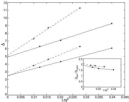
Figure 3: Energy gap as a function of $1/N^{2}$, where $N$ is the chain length. The upper two lines are for periodic boundary conditions, while the lower two lines are for open chains. Dashed and solid lines denote even and odd values of $N$ respectively. The inset shows the ratio $\Delta_{per}/\Delta_{open}$ as a function of $1/N^{2}$.

Next we consider the first excited state. Fig. 3 shows the energy gaps as a function of the chain length $N$, for chains with PBC (upper two lines) and for open chains (lower two lines). Although the results differ significantly between even and odd values of $N$, they extrapolate to about the same values for $N\to\infty$. We have fitted the gaps to the form $\Delta E(N)=\Delta E(\infty)+a/N^{2}$. The reason for this fitting form is that an excited state with a gap is expected to behave like a particle in a box white ; nakamura1 ; in a system of length $N$, the leading $N$-dependent term in the energy of such an object is $1/N^{2}$. The inset of Fig. 3 shows the ratio $\Delta_{per}/\Delta_{open}$ as a function of $1/N^{2}$ for even and odd values of $N$; the lines in the inset are obtained by taking the ratio of the fitted lines in the main figure.

In Table 1, we summarize the results shown in Fig. 3 by listing the gap for various values of $N$ for open ($\Delta_{open}$) and periodic ($\Delta_{per}$) boundary conditions as well as the ratio $\Delta_{per}/\Delta_{open}$. We see that the gap for the open chain extrapolates to a value of about $\Delta E=2.5$ which is not very different from the value of 2.38 obtained variationally in Eq. (28). Further, the gap for the chain with PBC extrapolates to a value which is about twice that of the open chain gap. This implies, for instance, that there is no bound state of two spin-1/2 excitations which has an energy which is significantly less than $2\Delta E$.

For open chains, we find that the total spin of the lowest excitation is $S_{tot}=1$ for even $N$ and $S_{tot}=2$ for odd $N$. The latter value can be understood as follows: If this excitation is the state (iii) discussed in Sec. II. B (see Fig. 2 (iii)), which interpolates between AKLT and a fully dimerized ground state, then it is possible to have an unpaired spin-1 at the edge of the fully dimerized side without costing any energy. This edge spin can combine with the spin-1/2 at the edge of the AKLT side and the spin-1/2 in the bulk to form $S_{tot}=2$.

$N$	$\Delta_{open}$	$\Delta_{per}$	$\Delta_{per}/\Delta_{open}$
5	6.08	9.28	1.53
6	6.29	11.28	1.79
7	4.34	7.09	1.63
8	4.63	8.72	1.88
9	3.61	6.30	1.75
10	3.82	7.29	1.91
$\infty_{odd}$	2.51	4.93	1.96
$\infty_{even}$	2.45	5.14	2.10

Table 1: Gaps for chains with open and periodic boundary conditions for different chain lengths. The last two lines give the gaps extrapolated to the thermodynamic limit for an odd and even number of sites respectively.

IV Generalizations

We can construct models involving higher spins or higher dimensions in which excitations in the bulk can carry spins which are a fraction of the spin at each site. We will discuss some examples below.

IV.1 Higher spin chains

The idea of a Hamiltonian with multiple ground states in which there are varying numbers of singlet bonds between neighboring sites can be generalized to higher spin chains. Consider a chain of spin-$S$ sites with a Hamiltonian such that all ground states must have at least $2S$ singlet bonds amongst every group of three neighboring sites. In analogy with Eq. (1), we can write such a Hamiltonian as $H=\sum h_{n}$, where $h_{n}$ is a sum of projection operators on to values of total spins ranging from $S+1$ to $3S$ for sites $n-1$, $n$ and $n+1$. A state in which there are $p$ singlet bonds between sites $2n-1$ and $2n$ and $2S-p$ singlet bonds between sites $2n$ and $2n+1$, for every value of $n$, is a ground state of such a Hamiltonian. In terms of the variables $u$ and $v$, such a state can be written as nakamura2

$$\Psi(p) = \prod_{n=-\infty}^{\infty}~{}[(u_{2n-1}v_{2n}-v_{2n-1}u_{2n})^{p}$$ (40)

$$~{}~{}~{}~{}~{}~{}~{}~{}(u_{2n}v_{2n+1}-v_{2n}u_{2n+1})^{2S-p}]~{}.$$

Now, each value of $p$ from 0 to $2S$ corresponds to a ground state of the Hamiltonian; hence there are $2S+1$ ground states. The case $S=1/2$ corresponds to the MG model majumdar , while the case $S=1$ corresponds to the model studied in Secs. II and III. The states in Eq. (40) have appeared in the literature as variational ground states of a dimerized spin-$S$ chain, with the integer $p$ changing as the dimerization parameter is varied nakamura2 .

One can now consider excitations which are ‘domain walls’ interpolating between ground states $\Psi(p_{1})$ on the left and $\Psi(p_{2})$ on the right, where, for instance, $p_{1}>p_{2}$. A state of this kind is

$$\Psi_{2n}(p_{1},p_{2})$$ (41)

$$= \prod_{m=-\infty}^{n-1}~{}[(u_{2m-1}v_{2m}-v_{2m-1}u_{2m})^{p_{1}}$$

$$~{}~{}~{}~{}~{}~{}\times~{}(u_{2m}v_{2m+1}-v_{2m}u_{2m+1})^{2S-p_{1}}]$$

$$~{}~{}~{}~{}~{}~{}\times~{}u_{2n-1}^{p_{1}-p_{2}}~{}\prod_{m=n}^{\infty}~{}[(u_{2m-1}v_{2m}-v_{2m-1}u_{2m})^{p_{2}}$$

$$~{}~{}~{}~{}~{}~{}\times~{}(u_{2m}v_{2m+1}-v_{2m}u_{2m+1})^{2S-p_{2}}]~{}.$$

This state has $S_{tot}^{z}=(p_{1}-p_{2})/2$ due to the factor of $u^{p_{1}-p_{2}}$ at site $2n-1$. We can now superpose states like this to form a momentum eigenstate, and calculate its variational energy. A similar procedure can be used to construct excited states interpolating between ground states with any two values of $p_{1}$ and $p_{2}$ lying in the range $0\leq p_{2}<p_{1}\leq 2S$. We thus see that the excited states of this spin-$S$ chain can have any value of the spin $(p_{1}-p_{2})/2$ going from 1/2 to $S$.

IV.2 Higher dimensional models

One can construct spin models in higher than one dimension in which the excited states exhibit spin fractionalization. Two examples are as follows.

(i) Consider a spin-1 model on a square lattice in which the Hamiltonian $H$ is a sum over Hamiltonians $H_{\square}$ of squares for which the ground state has at least two singlet bonds in each square cai ; $H_{\square}$ must be a sum of the projection operators $P_{3}$ and $P_{4}$ for the total spin of a square. The ground states of $H$ consist of a number of unbroken lines of singlet bonds such that each square has exactly two such lines running along two of its sides. Each line of singlet bonds can either extend all across the system or form a closed loop. In the limit of large system size $N$, the number of ground states grows as the exponential of $\sqrt{N}$. Hence the entropy per site vanishes at zero temperature, even though the number of ground states goes to infinity in the thermodynamic limit. Next, we can consider excited states in which one of the lines ends at a free spin 1/2 at one site; this leaves one square unsaturated. Two such excitations are shown in Fig. 4. One can then consider variational states in which the free spin 1/2 is allowed to move around the lattice in order to reduce its energy.

Figure 4: Spin-1/2 excitations in a square lattice. For PBC there has to be an even number of such excitations. The crosses mark the unsaturated squares which have less than two singlet bonds running along their sides.

(ii) Next we consider a spin-1 model on a triangular lattice in which the Hamiltonian $H$ is a sum over Hamiltonians $H_{\triangle}$ of triangles for which the ground state has at least two singlet bonds in each triangle; $H_{\triangle}$ must be the projection operator $P_{3}$ for the total spin of a triangle. The ground states of $H$ consist of unbroken lines of singlet bonds such that each triangle has exactly one line running along one of its sides. Once again, the number of ground states grows as the exponential of $\sqrt{N}$ for a system with $N$ sites. There are excited states in which one of the lines ends at a free spin 1/2 at one site; this leaves one triangle unsaturated. The free spin 1/2 can again move around so as to reduce its energy.

V Conclusions

We have introduced a Hamiltonian for a spin-1 chain which has three degenerate ground states, two of the MG type and one of the AKLT type. The lowest energy excitation carries spin-1/2 and interpolates between the AKLT state and one of the MG states; it has a gap $\Delta E\simeq 2.38J$. In the thermodynamic limit $N\to\infty$ and temperatures much lower than $\Delta E/k_{B}$, the system will consist of a dilute gas of the spin-1/2 excitations sen ; nakamura1 . Hence a quantity like the magnetic susceptibility will go as $\chi\sim\exp(-\beta\Delta E)$ at low temperatures. The spin-1/2 nature of these excitations can, in principle, be observed in ESR experiments.

Although the model has three ground states, they will not appear with equal weights in the limit of very low but non-zero temperature. Since the spin-1/2 excitations interpolate between the AKLT state and either one of the MG states, we expect that half the chain will be in the AKLT state, and a quarter will be in each of the two MG states. This implies that the structure factor $S(q)$ at very low temperatures will be given by $[S^{I}(q)+S^{III}(q)]/2$, where $S^{I}(q)$ and $S^{III}(q)$ are given in Eq. (11).

Finally, we have indicated how the spin-1 chain with spin-1/2 excitations can be generalized to both higher spins and higher dimensions. This provides one particular way of realizing the idea of spin fractionalization.

- (1)
- (2) F. D. M. Haldane, Phys. Lett. 93A, 464 (1983); Phys. Rev. Lett. 50, 1153 (1983).
- (3) W. J. L. Buyers, R. M. Morra, R. L. Armstrong, M. J. Hogan, P. Gerlach and K. Hirakawa, Phys. Rev. Lett. 56, 371 (1986).
- (4) J. P. Renard, M. Verdaguer, L. P. Regnault, W. A. C. Erkelens, J. Rossat-Mignod and W. G. Stirling, Europhys. Lett. 3, 945 (1987).
- (5) S. Ma, C. Broholm, D. H. Reich, B. J. Sternlieb and R. W. Erwin, Phys. Rev. Lett. 69, 3571 (1992).
- (6) M. P. Nightingale and H. W. J. Blöte, Phys. Rev. B 33, 659 (1986).
- (7) M. Takahashi, Phys. Rev. Lett. 62, 2313 (1989).
- (8) S. R. White and D. A. Huse, Phys. Rev. B 48, 3844 (1993).
- (9) I. Affleck, in Fields, Strings and Critical Phenomena, edited by E. Brezin and J. Zinn-Justin (North-Holland, Amsterdam, 1989).
- (10) E. Fradkin, Field Theories of Condensed Matter Systems (Addison-Wesley, Reading, 1991).
- (11) A. Auerbach, Interacting electrons and quantum magnetism (Springer-Verlag, New York, 1994).
- (12) G. Sierra, in Strongly Correlated Magnetic and Superconducting Systems, edited by G. Sierra and M. A. Martin-Delgado, Lecture Notes in Physics 478 (Springer, Berlin, 1997).
- (13) I. Affleck, T. Kennedy, E. H. Lieb and H. Tasaki, Comm. Math. Phys. 115, 477 (1988) and Phys. Rev. Lett. 59, 799 (1987).
- (14) A. Klümper, A. Schadschneider, and J. Zittartz, J. Phys. A 24, L955 (1991), and Europhys. Lett. 24, 293 (1993).
- (15) K. Okamoto and K. Nomura, Phys. Lett. A 169, 433 (1992).
- (16) R. Chitra, S. Pati, H.R. Krishnamurthy, D. Sen and S. Ramasesha, Phys. Rev. B 52, 6581 (1995).
- (17) E. Lieb, T. Schultz and D. Mattis, Ann. Phys. (N. Y.) 16, 407 (1961).
- (18) C. K. Majumdar and D. K. Ghosh, J. Math. Phys. 10, 1388 and 1399 (1969).
- (19) B. S. Shastry and B. Sutherland, Phys. Rev. Lett. 47, 964 (1981).
- (20) A. M. M. Pruisken, R. Shankar, and N. Surendran, Phys. Rev. B 72, 035329 (2005).
- (21) L. D. Faddeev and L. A. Takhtajan , Phys. Lett. A 85, 375 (1981).
- (22) D. A. Tennant, T. G. Perring, R. A. Cowley, and S. E. Nagler, Phys. Rev. Lett. 70, 4003 (1993).
- (23) P. W. Anderson, G. Baskaran, Z. Zou, and T. Hsu, Phys. Rev. Lett. 58, 2790 (1987).
- (24) X. G. Wen, Phys. Rev. B 44, 2664 (1991).
- (25) R. Coldea, D. A. Tennant, and Z. Tylczynski, Phys. Rev. B 68, 134424 (2003).
- (26) S. Yunoki and S. Sorella, Phys. Rev. Lett. 92, 157003 (2004).
- (27) D. P. Arovas, A. Auerbach, and F. D. M. Haldane, Phys. Rev. Lett. 60, 531 (1988).
- (28) W. J. Caspers, K. M. Emmett, and W. Magnus, J. Phys. A 17, 2687 (1984).
- (29) D. Sen, B. S. Shastry, R. E. Walstedt and R. Cava, Phys. Rev. B 53, 6401 (1996).
- (30) T. Nakamura and K. Kubo, Phys. Rev. B 53, 6393 (1996).
- (31) M. Nakamura and S. Todo, Phys. Rev. Lett. 89, 077204 (2002).
- (32) Z. Cai, S. Chen, S. Kou, and Y. Wang, cond-mat/0611170.