Distribution of spectral-flow gaps in the Rashba model
with disorder: a new universality

Abstract

We report a study of disordered electron systems with spin-orbit coupling on a cylinder using methods of random matrix ensembles. With a threading flux turned on, the single particle levels will generally avoid, rather than cross, each other. Our numerical study of the level-avoiding gaps in the disordered Rashba model demonstrates that the normalized gap distribution is of a universal form, independent of the random strength and the system size. For small gaps it exhibits a linear behavior, while for large gaps it decays exponentially. A framework based on matrix mechanical models is suggested, and is verified to reproduce the universal linear behavior at small gaps. Thus we propose to use the distribution of the spectral-flow gaps associated with flux insertion as a new way to characterize 2d random systems with spin-orbit coupling. The relevance and qualitative implications for spin (Hall) transport are also addressed.

Introduction In recent years, there is a surge of interests in doing spintronics, i.e. to manipulate and to control electron spins in solid state devices, with external electric, instead of magnetic, fields. Potential advantages include efficient generation of spin polarization inside the devices, handy manipulation of individual spins at nano-scales, and desired reduction of heat dissipation during information processing. (The last point is because, in particular, the electric field can induce a transverse spin Hall current, respecting time reversal invariance and therefore being dissipationless S.Murakami et al. (2003).) Since there is no fundamental direct coupling between spin and the electric field, the spin-orbit coupling (SOC) plays a central role in inducing the spin transport. For these reasons, the study of spin transport and, in particular, the spin Hall effect in systems with SOC has recently attracted much attention (for recent reviews, see e.g.E.I.Rashba (2006); H.-A.Engel et al. (2006)). In the literature, a mechanism for the spin transport due to SOC is called extrinsic or intrinsic, depending on whether disorder (such as impurities or imperfections) is involved or not. However, in a real sample there is always disorder; to study possible interplay between the intrinsic and extrinsic mechanisms, it is better to study them simultaneously in one unified framework, rather than to study them separately and add their contributions. In this paper we report such a study of the systems with SOC using the methods of random matrix ensembles.

A prototype of the intrinsic SOC is the Rashba coupling in a two dimensional electron gas. The intrinsic contribution J.Sinova et al. (2004) to the spin Hall conductivity in this model, which has a universal value $e/8\pi$, was found to be exactly cancelled by the extrinsic vertex contribution from impurities in a perturbative approach E.Mishchenko et al. (2004); J.I.Inoue et al. (2004). Naturally one asks whether the cancellation persists beyond perturbation theory, and if so whether this points to a new universality to be discovered in the disordered systems with SOC concerning the spin (Hall) transport. These are the questions we want to address.

We put the Rashba model with on-site randomness on a cylinder, and mimic an infinitesimal electric field by turning on slowly a magnetic flux threading the cylinder. The latter is equivalent to imposing a twisted phase in the boundary condition. The same technique has been used before in studying charge transport in the presence of localization Thouless (1974), as well as the integer R.B.Laughlin (1981) and fractional Q.Niu et al. (1985) quantum (charge) Hall effect. What we are concerned about here is the behavior of level-avoiding gaps due to disorder as the threading flux varies. (The relevance of the level-avoiding gaps to the transport has been discussed before in Refs. D.J.Thouless (1989) for the charge Hall effect and in Refs. D.N.Sheng et al. (2005); X.L.Qi et al. (2006); W.Q.Chen et al. (2005) for the spin Hall effect in this and similar models.) We have carried out a numerical study and indeed found a new universality in the random system with SOC. More concretely, the distribution of the (normalized) level-avoiding gaps is found to have a universal form, independent of both the random strength and the system size. It is linear at small gaps and decays exponentially at large gaps; and the average gap for un-normalized distribution seems to tend to a finite value when the system size becomes very large. In this paper we will suggest a matrix mechanical model for the underlying random ensemble, which is verified to exhibit the desired small-gap behavior. Usually one uses the level-spacing statistics as a characteristic of the universality in a random system or ensemble M.L.Mehta (1991). Here our results suggest a different type of characterization of random ensembles using the gap statistics in the spectral flow due to flux threading (or twisted boundary conditions).

The Disordered Rashba Model Consider the disordered Rashba model T.Ando (1989); D.N.Sheng et al. (2005) on a square lattice with size $L\times L$:

$$H=-t\sum_{\langle ij\rangle}c_{i}^{\dagger}c_{j}+\sum_{i}w_{i}c_{i}^{\dagger}c_{i}+V_{\rm SO}\left(i\sum_{i}c_{i}^{\dagger}\sigma_{x}c_{i+\hat{y}}-i\sum_{i}c_{i}^{\dagger}\sigma_{y}c_{i+\hat{x}}+{\rm h.c.}\right),$$ (1)

where $c_{i}=(c_{i\uparrow},c_{i\downarrow})$ are electron annihilation operators for up-spin and down-spin, respectively, $t$ the nearest-neighbor hopping, and $V_{\rm SO}$ the Rashba spin-orbit coupling. Disorder is represented by uniformly distributed on-site random potential $w_{i}\in[-W/2,W/2]$. We impose the free boundary conditions in $x$-direction and the twisted boundary conditions in $y$-direction: $\Psi(i,j+L)=e^{i\theta}\Psi(i,j)$, so that the model is put on a cylinder, which is threaded by a magnetic flux $\Phi=\hbar\theta/e$.

We diagonalize the Hamiltonian numerically. The basic parameters are $L$, $W$ and $V_{\rm SO}$. We have taken their ranges to be $L$=12, 14, 16, 18, 20, 24, 28, 32, 36, 40, 48 and $W=0.05t,0.1t,0.2t,0.4t,0.6t,0.8t,1.0t$, with the SOC fixed to be $V_{\rm SO}=0.5t$ unless stated otherwise. We can safely assume that our system is in the metallic phase, as the range of the randomness, $W$, is much less than the critical value ($W_{\rm c}=5.875t$ for $V_{\rm SO}=0.577t$) T.Ando (1989) for the insulating phase.

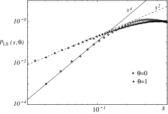
Figure 1: The level spacing distributions $p_{\rm LS}(s;\theta)$ for $\theta=0$ and $\theta=1$. $L=24$ and $W=0.2t$. For both data, the numbers of the level spacings we take are about $10^{6}$.

We have first calculated the level spacing distribution, $p_{\rm LS}(s;\theta)$ with $\theta$ fixed, where $s$ is the spacing between adjacent levels. Indeed we have seen a flux driven crossover from the symplectic to the unitary ensemble. Some typical results are shown in Fig. 1 for $\theta=0$ and $\theta=1$. We find the following power law behavior in the small-$s$ region,

$$p_{\rm LS}(s;\theta)\propto\left\{\begin{array}[]{ll}s^{4}&\mbox{for $\theta=0,\quad{\rm symplectic}$},\\ s^{2}&\mbox{for $\theta=1,\quad{\rm unitary}$},\end{array}\right.$$ (4)

in agreement with the random matrix ensembles with the corresponding symmetry M.L.Mehta (1991): When $\theta=0$, the system has time-reversal symmetry, leading to Kramer’s degeneracy, which is broken when $\theta\neq 0$.

Spectral-Flow Gap Distribution We are mainly interested in the spectral flow due to a varying flux. Typical level-flux diagrams are shown in Fig. 2.

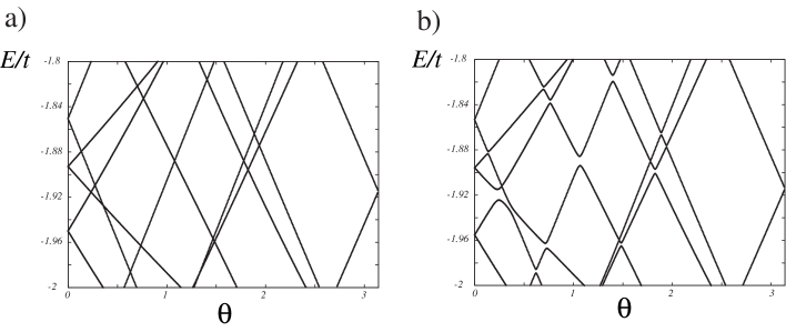
Figure 2: Level diagrams for $L=10$ a) without disorder ($W=0$) and b) with disorder ($W=0.1t$).

Without disorder (i.e. $W=0$), the energy levels cross each other as $\theta$ is varied (Fig. 2a), because momentum $k_{y}$ is a good quantum number. With $W\neq 0$, however, the translation symmetry in $y$-direction is broken by disorder, and generically gaps open near the would-be level-crossings (Fig. 2b). To characterize the spectral flow, one might try to extract from numerical data the statistical distribution of the level-avoiding gap $g$ which is, however, expected to depend on the parameters of the model. So a better way to detect whether there is universality is to plot the distribution $p_{\rm G}(\xi)$ of the normalized gap $\xi$, the value of $g$ normalized by the average $\langle g\rangle$: $\xi=g/{\langle g\rangle}$ with $L$ and $W$ fixed.

Our numerical data for a wide range of $L$ and $W$, as exemplified in Fig. 3a, demonstrates a remarkable universal behavior, namely the distribution, $p_{\rm G}(\xi)$, of the normalized gaps neither depends on $L$ nor $W$. Indeed the distribution is fit nicely by the following function:

$$p_{\rm G}(\xi)=\frac{a\xi^{2}}{{\rm sinh}(b\xi)},\quad{\rm with}\quad a=\frac{2b^{3}}{7\zeta(3)},\;\;b=\frac{\pi^{4}}{28\zeta(3)},$$ (5)

where $\zeta(z)$ is the zeta function, and constants $a$ and $b$ are fixed by the normalization conditions $\int_{0}^{\infty}d\xi p_{\rm G}(\xi)=1$ and $\int_{0}^{\infty}d\xi\xi p_{\rm G}(\xi)=1$. In Fig.3b, we show the data for the behavior of the distribution at large and small gaps: It is linear at small gaps and exponentially decays at large gaps.

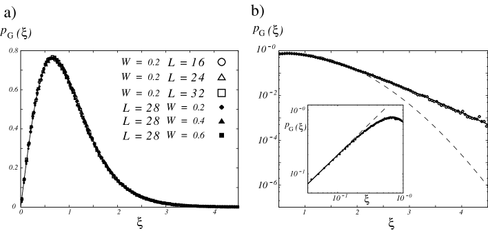
Figure 3: a) The gap distributions $p_{\rm G}(\xi)$ for various $L$ and $W$ (in units of $t$). The solid curve is the function (5). b) The gap distribution $p_{\rm G}(\xi)$ for $L=24$ and $W=0.2t$. For comparison, the function (5) (solid line) and the Gaussian unitary ensemble (GUE) surmise $(\pi\xi/2)e^{-\pi\xi^{2}/4}$ J.Zakrzewski et al. (1993)(dashed line) are also shown. The inset shows the small-$\xi$ behavior which can be fitted by a linear behavior $\propto\xi$ (dashed line). The number of gaps counted for each data point is greater than $5\times 10^{6}$.

To examine whether the SOC is crucial for the appearance of the universal behavior or not, we present in Fig.4 some data for the variance, $\sqrt{\sigma^{2}}=\sqrt{\int_{0}^{\infty}d\xi\xi^{2}p_{\rm G}(\xi)}$, of the normalized gap distribution with and without the SOC, respectively. While the data with $V_{\rm SO}=0.5t$ and $V_{\rm SO}=0.25t$ support a universal behavior, those with $V_{SO}=0$ clearly show non-universal $L$- and $W$-dependence.

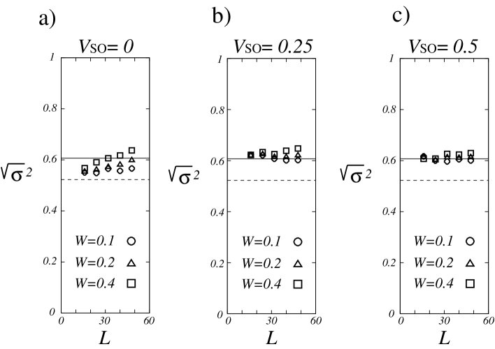
Figure 4: The variances $\sqrt{\sigma^{2}}$ of the gap distribution a) without and b, c) with SOC. For comparison the variance of the function (5)(solid line) and that of the GUE surmise (dashed line) are also shown.

Numerically we have also checked the large-$L$ behavior of the average gap $\langle g\rangle$, which is known to be non-universal. Figure 5a shows that it tends to a non-zero value as $L\to\infty$ with $W$ fixed. This fact is essential for the distribution of the normalized gap (5) to make sense in the thermodynamic limit. When combined with the Laughlin’s argument, it has a profound implication concerning spin Hall transport, which we are going to discuss below. In Fig.5b, we show the $W$-dependence of the limiting value $\langle g\rangle_{0}$; the solid curve is the following function, $\langle g\rangle_{0}=\alpha t\tanh\left(\beta\ln(\gamma W/t+1)\right)$ with $\alpha=2007.8$, $\beta=0.50$ and $\gamma=7.50$.

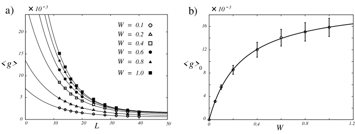
Figure 5: a) Non-universal behaviors of the average gaps $\langle g\rangle$. b) The $W$-dependence of the average gap in the limit $L\rightarrow\infty$.

New Universality of Random Ensembles The above-discovered universality of the distribution $p_{\rm G}(\xi)$ inspires us to search for the random ensemble underlying it. We notice that the spectral flow gaps we focus here are similar to the so-called avoided crossings that have been extensively studied in quantum chaos (see, e.g.Haake (2001)). Our model contains a periodic (flux) parameter $\theta$ in the twisted boundary condition. Since time reversal invariance is respected only for $\theta=0$ and $\pi$, our system should correspond to a random ensemble with unitary symmetry except at $\theta=0$ and $\pi$, near which there are crossovers to symplectic symmetry. The distribution of avoided crossings for Gaussian unitary ensembles (GUE) was studied before in the literature of quantum chaos Haake (2001). In Fig.3b, we show the comparison of our data with the GUE surmise given in Ref. J.Zakrzewski et al. (1993). Though the linear behavior in the small-$\xi$ region agrees with the GUE studied in Refs. M.Wilkinson (1989); E.J.Austin and M.Wilkinson (1992), the exponential decay in the large-$\xi$ region certainly does not J.Zakrzewski et al. (1993). Since the spectral flow is due to a varying parameter $\theta$, a more natural setting should be a matrix quantum mechanical model B.D.Simons et al. (1993), in which the time variable $t$ may be identified with $\theta$. Below let us show that in a wide class of matrix mechanical models, the distribution $p_{\rm G}(\xi)$ is indeed linear at small gaps and is independent of either the size of matrices or the potential in the model. The Lagrangian of the models we consider is

$$L=\frac{1}{2}{\rm Tr}\dot{\Phi}(t)^{2}+{\rm Tr}V(\Phi(t))\ ,$$ (6)

where $\Phi(t)$ is an $N\times N$ Hermitian matrix, and ${\rm Tr}V(\Phi)$ a potential invariant under the automorphism $\Phi\rightarrow G\Phi G^{\dagger}$ with $G$ unitary. Writing $\Phi(t)=U(t)^{\dagger}{\rm diag}(\lambda_{1}(t),\cdots\lambda_{N}(t))U(t)$ in terms of its eigenvalues $\lambda_{i}(t)$ and the unitary matrix $U(t)$ that diagonalizes it, the Lagrangian is recast into

$$L=\sum_{i}\frac{1}{2}\dot{\lambda}^{2}_{i}+\sum_{i<j}\left|\lambda_{i}-\lambda_{j}\right|^{2}\omega_{ij}\omega_{ji}+\sum_{i}V(\lambda_{i})$$ (7)

with $\omega=iU\dot{U}^{\dagger}$. The corresponding Hamiltonian is

$$H=\frac{1}{2}\sum_{i}p_{i}^{2}+\sum_{i}V(\lambda_{i})+\sum_{i<j}\frac{L_{ij}L_{ji}}{|\lambda_{i}-\lambda_{j}|^{2}},$$ (8)

where $p_{i}$ and $L_{ij}$ are the conjugate momenta of $\lambda_{i}$ and $\omega_{ji}$, respectively. The statistical properties are determined by the Gibbs measure,

$$dG_{N}=\frac{1}{{\cal Z}_{N}}e^{-\beta H}\prod_{i}d\lambda_{i}dp_{i}\prod_{i<j}dL_{ij}dL_{ij}^{*},$$ (9)

where ${\cal Z}_{N}$ is the normalization constant. The un-normalized gap distribution $n(g)$ is given by

$$n(g)=N(N-1)\prod_{k=3}^{N}\int_{g/2<|\lambda_{k}|}dG_{N}\sum_{n}\delta(t-t_{n})\delta(-g/2-\lambda_{1})\delta(g/2-\lambda_{2}),$$ (10)

where $t_{n}$ denotes a level avoiding point between $\lambda_{1}$ and $\lambda_{2}$. See Fig.6.

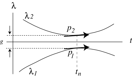
Figure 6: An avoiding gap between $\lambda_{1}$ and $\lambda_{2}$.

From the normalization condition, the gap distribution is obtained by

$$p_{\rm G}(\xi)=\langle g\rangle n(g)\left(\int dgn(g)\right)^{-1}.$$ (11)

At the level avoiding points $t=t_{n}$, we have $p_{1}=p_{2}$ with $\dot{p_{2}}-\dot{p_{1}}>0$. Thus $\sum_{n}\delta(t-t_{n})$ in the integral can be replaced with

$$\sum_{n}\delta(t-t_{n}) = \delta(p_{2}-p_{1})(\dot{p}_{2}-\dot{p}_{1}+|\dot{p}_{2}-\dot{p}_{1}|)/2$$ (12)

$$= -\delta(p_{2}-p_{1})\left(\frac{\partial H}{\partial(\lambda_{2}-\lambda_{1})}-\left|\frac{\partial H}{\partial(\lambda_{2}-\lambda_{1})}\right|\right),$$

where we have used the equations of motion for $p_{1}$ and $p_{2}$. While the resulting integral is hard to perform, the small-$g$ behavior can be easily seen to be

$$n(g)=Ag,$$ (13)

where $A$ is a constant given by

$$A=\frac{4N(N-1)}{\beta{\cal Z}_{N}}\prod_{i=1}^{N}\int dp_{i}\prod_{i<j}\int d\tilde{L}_{ij}\int d\tilde{L}_{ij}^{*}\prod_{k=3}^{N}\int d\lambda_{k}\prod_{2<k<l}(\lambda_{k}-\lambda_{l})^{2}\prod_{k=3}^{N}\lambda_{k}^{4}$$

$$\times\delta(p_{2}-p_{1})\exp\left[-\beta\left(\sum_{i=1}^{N}\frac{p_{i}^{2}}{2}-\sum_{i<j}\tilde{L}_{ij}\tilde{L}_{ji}-\sum_{k=3}^{N}V(\lambda_{k})-2V(0)\right)\right].$$ (14)

Thus we have a universal linear behavior for $p_{\rm G}(\xi)$ in the small-$\xi$ region for any $N\geq 2$. The insensibility of the linear behavior to the number of levels $N$ coincides with that to $L$ for the Rashba model as the number of levels of the Rashba model is given by $2L^{2}$.

We note that the large-$\xi$ behavior of the random matrix quantum mechanics does depend on the form of the potential $V(\lambda)$. This is well-known for usual random matrix ensembles. For example, for polynomial potentials, the kernel of the unitary ensembles in the large $N$ limit has a universal form corresponding to the Gaussian ensembleE.Brézin and Zee (1993):

$$K(x,y)=\frac{\sin\pi(x-y)}{\pi(x-y)};$$ (15)

but for logarithmically growing potentials, $V(\lambda)\sim\frac{1}{2a}(\ln\lambda)^{2}\quad(\lambda\gg 1)$, it shows another universality K.A.Muttalib et al. (1993):

$$K(x,y)=\frac{a}{\pi}\frac{\sin\pi(x-y)}{\sinh a(x-y)}.$$ (16)

It is plausible that there exists a class of potentials in matrix mechanical models, which reproduce the spectral-flow gap statistics we have found from our numerical calculations.

Spectral-Flow Gaps and the Hall Transport In the above we have studied the distribution of spectral-flow gaps in a disordered system with SOC, as a response to twisted boundary conditions. This is in line with the Laughlin gauge argument R.B.Laughlin (1981) for the charge Hall effect, which has been recently adapted to the case of the spin Hall effect D.N.Sheng et al. (2005); X.L.Qi et al. (2006); W.Q.Chen et al. (2005) for systems with SOC. Our data show no level crossing in the spectral flow, in agreement with Refs. D.N.Sheng et al. (2005); W.Q.Chen et al. (2005) for the disordered models. Because of level avoiding, each level always flows back to its original energy after the flux adiabatically increases from zero to the unit flux quantum. In contrast to the quantum (charge) Hall effect, in the present case the system is in the metallic phase, and there are levels going across the Fermi level. At absolute zero temperature and in the adiabatic limit, the levels that are below the Fermi level and never go across it will maintain its own contribution to the spin Hall conductivity, similar to the case of the charge Hall effect. The sum of these levels to the spin Hall conductivity of the system is expected generically to have zero expectation value if the position of the Fermi level is set randomly. However, during the adiabatic variation of the flux, the instantaneous spin Hall conductivity will fluctuate because of the levels that move out of or dive into the Fermi surface. So at least for the cylindrical geometry, the time-averaged spin Hall conductivity should be very small, compared to the clean intrinsic limit.

Moreover, a finite electric field will induce the transition across the Fermi surface between levels with sufficiently small gaps (Landau-Zener-like tunneling). Also at finite temperature, thermal fluctuations will cause similar transitions between levels with gaps smaller than the average thermal energy. Therefore, the fluctuations in spin Hall conductivity may be significant if the temperature is not too low and the applied electric field is not too small. It is no doubt that the knowledge we obtained in this paper on the distribution of level-avoiding gaps and on the magnitude of the average gap will be useful for detailed analyses of the disorder effects on the fluctuations in spin Hall conductivity. Here we only point out some features inferred from our results. First, the level avoiding gap distribution is of a universal form for the normalized gap, which is linear at small gaps. So we expect that there is also a universality in the fluctuations in $\sigma^{\rm spin}_{\rm H}$ if properly scaled. In other words, the fluctuations may have a one-parameter scaling law by the average gap at sufficiently low temperature, where the Landau-Zener tunneling is dominating. Second, since the average gap is non-vanishing in the large-$L$ limit, we expect that the fluctuations in $\sigma^{\rm spin}_{\rm H}$ will be governed by an exponential factor involving the temperature or the electric field over the average gap.

Summary and Discussions In this paper, we examined the distributions of level avoiding gaps in the Rashba model in the presence of disorder. We found that the normalized distribution is of a universal form, independent of the random strength and the system size, while the average value of the gaps is non-universal.

A natural expectation is that our universal distribution works for other models with SOC. (For example, a disordered two-dimensional electron gas with Dresselhaus SOC Mal’shukov and Chao (2005), a generalized Rashba model Nomura et al. (2005), a graphene model with SOC C.L.Kane and E.J.Mele (2005), and a two dimensional hole gas B.A.Bernevig and Zhang (2005).) We note that this does not mean the spin Hall conductivity itself is universal: It depends on the average value of the level-avoiding gaps, thus it could be model dependent. For example, if the average value becomes zero in the thermodynamic limit, a net spin Hall effect can be observed. In addition, what we discuss in the spectral flow argument is not the spin Hall current itself but the spin accumulation after the unit flux insertion. Because the spin is not conserved in general, these two quantities are not necessarily in accordance with each other. This also supports the expectation that systems with different spin Hall conductivities may have the universal gap distribution we discovered.

In the absence of disorder the Rashba model has integrability of the momentum conservation which is the origin of the level crossings. The integrability may explain a mixed behavior of our distribution between the Poisson distribution and the GUE one. Indeed, it is known that the gap distributions for fully chaotic systems without integrability show no mixed behavior and are in good agreement with the GUE surmise J.Zakrzewski et al. (1993).

To conclude, we remark that the new universality we discovered in this paper may have consequences concerning quantum transport in mesoscopic systems with SOC. It may also provide helpful insight into the interplay between localization and SOC in the spin Hall effect of disordered systems.

Acknowledgments The computation in this work has been done using the facilities of the Supercomputer Center, Institute for Solid State Physics, University of Tokyo. The discussions with E. Mishchenko, D.N. Sheng, Z.Y.Weng and M.Wilkinson are acknowledged. Y.S.Wu is supported in part by the U.S. NSF through grant No. PHY-0407187. This work was begun in summer 2005, when he visited the ISSP, University of Tokyo. He thanks the host institution for the financial support and warm hospitality.

References

- S.Murakami et al. (2003) S.Murakami, N.Nagaosa, and S.C.Zhang, Science 301, 1348 (2003).
- E.I.Rashba (2006) E.I.Rashba, Physica E 34, 31 (2006).
- H.-A.Engel et al. (2006) H.-A.Engel, E.I.Rashba, and B.I.Halperin, arXiv. cond-mat/0603306 (2006).
- J.Sinova et al. (2004) J.Sinova, D.Culcer, Q.Niu, N.A.Sinitsyn, T.Jungwirth, and A.H.MacDonald, Phy. Rev. Lett. 92, 126603 (2004).
- E.Mishchenko et al. (2004) E.Mishchenko, A.V.Shytov, and B.I.Halperin, Phys. Rev. Lett. 93, 226602 (2004).
- J.I.Inoue et al. (2004) J.I.Inoue, B.E.W.Bauer, and L.W.Molenkamp, Phys. Rev. B 70, 041303 (2004).
- Thouless (1974) D. Thouless, Phys. Rep. 13, 93 (1974).
- R.B.Laughlin (1981) R.B.Laughlin, Phys. Rev. B 23, R5632 (1981).
- Q.Niu et al. (1985) Q.Niu, D.J.Thouless, and Y.S.Wu, Phys. Rev. B 31, 3372 (1985).
- D.J.Thouless (1989) D.J.Thouless, Phys. Rev. B 40, 12034 (1989).
- D.N.Sheng et al. (2005) D.N.Sheng, L.Sheng, Z.Y.Weng, and F.D.M.Haldane, Phys. Rev. B 72, 153307 (2005).
- X.L.Qi et al. (2006) X.L.Qi, Y.S.Wu, and S.C.Zhang, Phys. Rev. B 74, 085308 (2006).
- W.Q.Chen et al. (2005) W.Q.Chen, Z.Y.Weng, and D.N.Sheng, Phys. Rev. B 72, 235315 (2005).
- M.L.Mehta (1991) M.L.Mehta, Random Matrices (Academic Press, 1991), 2nd ed.
- T.Ando (1989) T.Ando, Phys. Rev. B 40, 5325 (1989).
- J.Zakrzewski et al. (1993) J.Zakrzewski, D.Delande, and M.Kuś, Phys. Rev. E 47, 1665 (1993).
- Haake (2001) F. Haake, Quantum Signatures of Chaos (Springer, 2001), 2nd ed.
- M.Wilkinson (1989) M.Wilkinson, J. Phys. A 22, 2795 (1989).
- E.J.Austin and M.Wilkinson (1992) E.J.Austin and M.Wilkinson, Nonlinearity 5, 1137 (1992).
- B.D.Simons et al. (1993) B.D.Simons, P.A.Lee, and B.L.Altshuler, Phys. Rev. Lett. 72, 64 (1993).
- E.Brézin and Zee (1993) E.Brézin and A. Zee, Nucl. Phys. B 402, 613 (1993).
- K.A.Muttalib et al. (1993) K.A.Muttalib, Y.Chen, M.E.H.Ismail, and V.N.Nicopoulos, Phys. Rev. Lett. 71, 471 (1993).
- Mal’shukov and Chao (2005) A. Mal’shukov and K. A. Chao, Phys. Rev. B 71, 121308(R) (2005).
- Nomura et al. (2005) K. Nomura, J. Sinova, N. Sinitsyn, and A.H.MacDonald, Phys. Rev. B 72, 165316 (2005).
- C.L.Kane and E.J.Mele (2005) C.L.Kane and E.J.Mele, Phys. Rev. Lett. 95, 226801 (2005).
- B.A.Bernevig and Zhang (2005) B.A.Bernevig and S. Zhang, Phys. Rev. Lett. 95, 016801 (2005).