Intensive thermodynamic parameters in nonequilibrium systems

Abstract

Considering a broad class of steady-state nonequilibrium systems for which some additive quantities are conserved by the dynamics, we introduce from a statistical approach intensive thermodynamic parameters (ITPs) conjugated to the conserved quantities. This definition does not require any detailed balance relation to be fulfilled. Rather, the system has to satisfy a general additivity property, which holds in most of the models usually considered in the literature, including those described by a matrix product ansatz with finite matrices. The main property of these ITPs is to take equal values in two subsystems, making them a powerful tool to describe nonequilibrium phase coexistence, as illustrated on different models. We finally discuss the issue of the equalization of ITPs when two different systems are put into contact. This issue is closely related to the possibility of measuring the ITPs using a small auxiliary system, in the same way as temperature is measured with a thermometer, and points at one of the major difficulties of nonequilibrium statistical mechanics. In addition, an efficient alternative determination, based on the measure of fluctuations, is also proposed and illustrated.

I Introduction

The general concept of intensive thermodynamic parameters plays a crucial role in equilibrium statistical mechanics. For systems in contact, ITPs like temperature, pressure or chemical potential equalize their values once the equilibrium state is reached, provided that their associated quantities, energy, volume or number of particles, can be exchanged. Since this property holds even in the case of systems that exhibit different microscopic dynamics, this equalization became the key criterion in equilibrium statistical mechanics to study the influence of the environment on a given system, for example when a reservoir is connected to it. Moreover the theory of phase coexistence as well as the measurement of, for instance, temperature with a thermometer draw on this powerful concept.

Indeed this potency of the ITP formalism motivates the endeavor to generalize the notion of ITPs to nonequilibrium systems. There exist several different approaches mostly focusing on the generalization of temperature out of equilibrium. For stationary nonequilibrium systems that fulfill a local equilibrium condition, equilibrium properties are locally recovered, so that ITPs can be naturally defined on macroscopic scales that remain small in comparison with the system size deGroot . Beyond local equilibrium, more phenomenological endeavors based on thermodynamical grounds Jou have been proposed, as well as statistical approaches illustrated on some specific models Puglisi ; MaxEnt ; Hatano ; BDD ; Jou06 . Finally, in the case of non-stationary slow dynamics, a notion of temperature may be derived from a generalized fluctuation-dissipation relation (FDR) CuKuPe ; Kurchan ; Crisanti ; Ritort in analogy to equilibrium statistical mechanics. Still, in spite of these numerous propositions, the relevance of this concept of effective temperature and its possible generality have been barely discussed.

Besides, other notions of ITPs have appeared in the recent literature on nonequilibrium systems. For instance, in the context of stochastic models with a conserved mass $M$ (or number of particles), like the Zero Range Process or different kinds of mass transport models Evans-Rev05 , a formal grand-canonical ensemble has been defined, in which systems with a total mass $M$ appear with a probability weight proportional to $\exp(-\mu M)$, $\mu$ being called a chemical potential. We call this ensemble a “formal” one, since no definition of the chemical potential is given prior to the grand-canonical construction, and no physical mechanism allowing for fluctuations of the total mass (like, e.g., a contact with a reservoir) is described. Hence, the grand-canonical distributions introduced so-far appear more as mathematical tools with interesting properties, as it may be considered as a Laplace transform with respect to $M$ of the canonical distribution for which $M$ is fixed Arndt ; Evans-Rev05 . Even more importantly, if this formal grand-canonical ensemble was to be considered as defining the chemical potential, nothing could be said from it on the possible equalization of this parameter between two subsystems of a globally isolated system, since in the grand-canonical ensemble, the chemical potential is externally imposed.

The aim of the present work is to introduce a precise and general theoretical background allowing for the definition of ITPs conjugated to conserved quantities in nonequilibrium systems. Note that the systems considered here are out of equilibrium not due to the presence of gradients imposed, for instance, by boundary reservoirs, but because of the breaking of microreversibility (that is, time-reversal invariance) at the level of the microscopic dynamics in the bulk. Accordingly, the ITPs are not space dependent, as would be the case for systems that fulfill the local equilibrium assumption. We state the hypotheses underlying the present construction, and clarify the physical interpretation of the grand-canonical ensemble. We then discuss the relevance and usefulness of the concept of ITP, with particular emphasis on the description of phase coexistence. Although the proposed generalization of ITPs appears to be rather natural, it turns out that non-trivial problems arise as soon as systems with different dynamics are put into contact. This issue is essential if one wants to measure an ITP using a small auxiliary system –just like temperature is measured with a thermometer– and points at one of the main difficulties of nonequilibrium statistical mechanics. Note that part of the results reported here have appeared in a short version short .

The paper is organized as follows. Sec. II introduces the concept of intensive thermodynamic parameters in the framework of nonequilibrium systems. The main condition of validity for this concept is given and some features in analogy to equilibrium statistical physics are discussed. Further the applicability of the definition for systems described with matrices (either matrix product ansatz or transfer matrix method) is studied, and an illustration of this approach on two simple models is given. Sec. III is dedicated to the issue of phase separation, specifically the problem of condensation, in different models. We show how the concept of ITPs could improve the understanding of phase separation in these kind of models. Finally, the contact of two systems with different dynamics is investigated in Sec. IV, with emphasis on the issue of equalization of ITPs. We also explore possible ways of determining the ITPs in experiments or numerical simulations.

II Nonequilibrium intensive thermodynamic parameters

II.1 Framework and definitions

Let us start by considering a general macroscopic system that exhibits a steady state, and such that the dynamics conserves some additive quantities, referred to as $Q_{k}$, $k=1,\ldots,\ell$, in the following. Such systems have been extensively studied for instance in the context of markovian stochastic models, and simple examples include the zero-range process (ZRP) Evans-Rev05 , more general mass transport models Zia04 ; Zia05 ; Evans06 , or the asymmetric exclusion process (ASEP) in a closed geometry Arndt . On the microscopic level, the nonequilibrium character of the dynamics manifests itself (apart from the lack of detailed balance) in the presence of a non-trivial dynamical weight $f_{\alpha}$ associated with each microscopic configuration $\alpha$, in the steady-state probability $P_{\alpha}$. More precisely, the latter reads

$$P_{\alpha}=\frac{f_{\alpha}}{Z(Q_{1},\ldots,Q_{\ell})}\prod_{k=1}^{\ell}\delta(Q_{k}^{\alpha}-Q_{k})\,,$$ (1)

where the product of delta distributions ensures the conservation of the quantities $Q_{k}$. The function

$$Z(Q_{1},\ldots,Q_{\ell})=\sum_{\alpha}f_{\alpha}\prod_{k=1}^{\ell}\delta(Q_{k}^{\alpha}-Q_{k})$$ (2)

serves as normalization factor, which will be referred to as “partition function” in analogy to equilibrium statistical mechanics. Let us emphasize that in equilibrium systems, the probability weight $f_{\alpha}$ is either a constant independent of $\alpha$, or an exponential factor accounting for the exchange of a conserved quantity with a reservoir. For instance, in the equilibrium canonical ensemble, the conserved quantity would be the number of particles, whereas $f_{\alpha}$ would be the Gibbs factor $\exp(-\beta E_{\alpha})$, where $E_{\alpha}$ is the energy of configuration $\alpha$, and $\beta$ is the inverse temperature. On the contrary, in a nonequilibrium system, the weights $f_{\alpha}$ also account for purely dynamical effects related to the absence of microreversibility (the latter being deeply rooted in the hamiltonian properties of equilibrium systems), so that these weights generically depart from a constant, even if no conserved quantity is exchanged with a reservoir.

To introduce a definition for ITPs in nonequilibrium situations, we first recall that their equilibrium definition is related to the exchanges of conserved quantities between subsystems, and ensures the equality of ITPs in different parts of the system. Following the same line of thought in a nonequilibrium context, let us divide our system, in an arbitrary way, into two subsystems $\mathcal{S}_{a}$ and $\mathcal{S}_{b}$. The sum $Q_{ka}$+$Q_{kb}=Q_{k}$ is kept constant due to the conservation law, whereas exchanges of these quantities between the two subsystems are allowed. The microstate $\alpha$ is now defined as the combination of the two microstates $\{\alpha_{a},\alpha_{b}\}$ of the subsystems, so that the probability of a microstate is denoted as $P_{\alpha_{a},\alpha_{b}}$. An important quantity in the following approach is the conditional probability $\Psi(Q_{1a},\ldots,Q_{\ell a}|Q_{1},\ldots,Q_{\ell})$ that the conserved quantities have values $Q_{ka}$ in subsystem $\mathcal{S}_{a}$, given their total values $Q_{k}$

$$\Psi(\{Q_{ka}\}|\{Q_{k}\})=\sum_{\alpha_{a},\alpha_{b}}P_{\alpha_{a},\alpha_{b}}\prod_{k=1}^{\ell}\delta(Q_{ka}^{\alpha_{a}}-Q_{ka})\,.$$ (3)

The key assumption in the following derivation is that the logarithm of $\Psi(\{Q_{ka}\}|\{Q_{k}\})$ satisfies an asymptotic additivity property, namely

$$\ln\Psi(\{Q_{ka}\}|\{Q_{k}\}) = \ln Z_{a}(\{Q_{ka}\})+\ln Z_{b}(\{Q_{k}-Q_{ka}\})$$ (4)

$$- \ln Z(\{Q_{k}\})+\epsilon_{N}(\{Q_{ka}\},\{Q_{k}\})$$

with

$$|\epsilon_{N}(\{Q_{ka}\},\{Q_{k}\})|\ll|\ln\Psi(\{Q_{ka}\}|\{Q_{k}\})|\;,$$ (5)

in the thermodynamic limit $N\to\infty$. In Eq. (4), $Z_{\nu}(\{Q_{k\nu}\})$ refers to the isolated subsystem $\mathcal{S}_{\nu}$, $\nu\in\{a,b\}$, and N is the number of degrees of freedom. That this additivity condition is fulfilled for some rather large classes of nonequilibrium systems will be illustrated in the following examples.

Some of the simplest systems that fulfill Eqs. (4), (5) are lattice models with a factorized steady state distribution (where sites are labelled by $i=1,\dots,N$, and $\alpha=\{\alpha_{i}\}$)

$$P_{\alpha}=\frac{1}{Z(Q_{1},\ldots,Q_{\ell})}\prod_{i=1}^{N}f_{i,\alpha_{i}}\prod_{k=1}^{l}\delta\left(\sum_{i=1}^{N}Q_{ki}^{\alpha_{i}}-Q_{k}\right)\;,$$ (6)

in which case the term $\epsilon_{N}$ vanishes. Well-known examples of models with factorized steady-states are for instance the ZRP Evans-Rev05 and other general mass transport models Zia04 ; Zia05 . Accordingly, the physical interpretation of the additivity condition given in Eqs. (4), (5) is that, on large scale, the system behaves essentially as if the probability weight was factorized, although the genuine probability weight may not be factorized.

As mentioned above, our aim is to define a parameter that takes equal values within the two (arbitrary) subsystems $\mathcal{S}_{a}$ and $\mathcal{S}_{b}$. Guided by the equilibrium procedure, we consider the most probable value of $Q_{ka}$, denoted by $Q_{ka}^{*}$, which maximizes the probability $\Psi(\{Q_{ka}\}|\{Q_{k}\})$. This most probable value satisfies

$$\frac{\partial\ln\Psi(\{Q_{ka}\}|\{Q_{k}\})}{\partial Q_{ka}}\Big{|}_{Q_{ka}^{*}}=0\,.$$ (7)

Using the additivity condition (4), (5), we obtain the following relation

$$\frac{\partial\ln Z_{a}}{\partial Q_{ka}}\Big{|}_{Q_{ka}^{*}}=\frac{\partial\ln Z_{b}}{\partial Q_{kb}}\Big{|}_{Q_{k}-Q_{ka}^{*}}.$$ (8)

Hence, it is natural to define the ITP $\lambda_{k}$ conjugated to the conserved quantity $Q_{k}$ in a nonequilibrium system as

$$\lambda_{k}\equiv\frac{\partial\ln Z}{\partial Q_{k}}\;,\qquad k=1,\dots,\ell\;.$$ (9)

Once the steady state is reached, this quantity equalizes in the two subsystems $\mathcal{S}_{a}$ and $\mathcal{S}_{b}$ due to Eq. (8), and thus satisfies the basic requirement for the definition of an ITP.

Actually, for the approach to be fully consistent, one has to check that the value of $\lambda_{k}$ does not depend on the choice of the partition, as long as both subsystems remain macroscopic. We show in Appendix A that this is indeed the case, at least under the assumption (which is consistent with the additivity condition) that $\ln Z$ is extensive. To achieve this result one shows that the ITP $\lambda_{k}$ obtained from the subsystems is equal to the global ITP defined on the whole system from Eq. (9), independently of the partition chosen (see Appendix A). Thus from now on, we compute the ITP $\lambda_{k}$ using Eq. (9) for the whole system.

II.2 Nonequilibrium “grand-canonical” ensemble

Now that we have defined the notion of ITP, it is natural to try to introduce a grand-canonical ensemble describing a system in contact with a reservoir of conserved quantities, that imposes its values of $\{\lambda_{k}\}$ to the system. Let us consider a partition of a large isolated system into two subsystems $\mathcal{S}_{a}$ and $\mathcal{S}_{b}$, such that one of the macroscopic systems is much smaller than the other. The larger subsystem, say $\mathcal{S}_{b}$, serves as a reservoir for the $\{Q_{k}\}$, leading to a natural definition of a “grand-canonical” distribution. This distribution is obtained by integrating the “canonical” distribution (1) over the degrees of freedom of the reservoir

$$\tilde{P}_{\alpha_{a}} = \frac{f_{\alpha_{a}}}{Z(Q_{1},\ldots,Q_{\ell})}\sum_{\alpha_{b}}f_{\alpha_{b}}\prod_{k=1}^{\ell}\delta(Q_{ka}^{\alpha_{a}}+Q_{kb}^{\alpha_{b}}-Q_{k})$$ (10)

$$= \frac{f_{\alpha_{a}}}{Z(Q_{1},\ldots,Q_{\ell})}Z_{b}(\{Q_{k}-Q_{ka}^{\alpha_{a}}\})$$

Note that in the above equation, we assume the factorization property $f_{\alpha_{a},\alpha_{b}}=f_{\alpha_{a}}f_{\alpha_{b}}$, that is we neglect possible boundary contributions, similarly to the assumptions often made in the equilibrium context. Expanding the logarithm of the partition function $Z_{b}$ for $Q_{ka}^{\alpha_{a}}\ll Q_{k}$, one finds to leading order in $Q_{ka}^{\alpha_{a}}$

$$\ln Z_{b}(\{Q_{k}-Q_{ka}^{\alpha_{a}}\}) \approx \ln Z_{b}(\{Q_{k}\})-\sum_{k=1}^{\ell}\frac{\partial\ln Z_{b}}{\partial Q_{kb}}\Big{|}_{Q_{k}}Q_{ka}^{\alpha_{a}}$$ (11)

$$\approx \ln Z_{b}(\{Q_{k}\})-\sum_{k=1}^{\ell}\lambda_{k}Q_{ka}^{\alpha_{a}}\;,$$

where we approximated

$$\frac{\partial\ln Z_{b}}{\partial Q_{kb}}\Big{|}_{Q_{k}}\approx\frac{\partial\ln Z_{b}}{\partial Q_{kb}}\Big{|}_{Q_{kb}^{*}}=\lambda_{k}\;.$$ (12)

This is justified in the limit $N_{a}/N\to 0$. Therefore we obtain for the “grand-canonical” distribution the following expression

$$\tilde{P}_{\alpha_{a}}=\frac{f_{\alpha_{a}}}{\tilde{Z}(\lambda_{1},\ldots,\lambda_{\ell})}\,\exp\left(-\sum_{k=1}^{l}\lambda_{k}Q_{ka}^{\alpha_{a}}\right)\;.$$ (13)

which defines the grand-canonical partition function

$$\tilde{Z}(\lambda_{1},\ldots,\lambda_{\ell})=\sum_{\alpha_{a}}f_{\alpha_{a}}\,\exp\left(-\sum_{k=1}^{l}\lambda_{k}Q_{ka}^{\alpha_{a}}\right)\;.$$ (14)

Interestingly, the cumulants $<Q_{k_{1}}Q_{k_{2}}\cdots Q_{k_{n}}>_{c}$ may be expressed as a derivative of the logarithm of the grand-canonical partition function $\tilde{Z}(\{\lambda_{k}\})$, which thus appears as the associated generating function, as follows:

$$<Q_{k_{1}}Q_{k_{2}}\cdots Q_{k_{n}}>_{c} = (-1)^{n}$$

$$\frac{\partial}{\partial\lambda_{k_{1}}}\frac{\partial}{\partial\lambda_{k_{2}}}\cdots\frac{\partial}{\partial\lambda_{k_{n}}}\ln\tilde{Z}(\{\lambda_{k}\})$$

Note that some of the indices among $k_{1},\ldots,k_{n}$ may be the same. This result generalizes the corresponding well-known equilibrium result Fulde . Accordingly, checking the validity of such relations in a given system does not show that microstates compatible with the constraints are equiprobable, contrary to what is sometimes implicitely assumed (e.g., in the context of granular matter Swinney ).

II.3 Applicability for nonfactorized steady states

As stated above every nonequilibrium system that exhibits a product measure automatically fulfills the additivity property given in Eqs. (4), (5), since $\epsilon_{N}$ vanishes in this case. The aim of this section is to discuss some typical cases for which the steady-state distribution does not factorize, but still satisfies the additivity condition. As a result, the ITP framework is relevant for such systems. There are two important classes of models with nonfactorized steady states: systems where the stationary state can be expressed by a matrix product ansatz, and models described by a transfer matrix.

II.3.1 Matrix product ansatz

Practically speaking, considering a matrix product ansatz means that, in a one-dimensional system with periodic boundary conditions, one expresses the probability weight $f_{\alpha}$ in the form

$$f_{\alpha}=\mathrm{Tr}\prod_{i=1}^{N}M_{\alpha_{i}}$$ (16)

where $M_{\alpha_{i}}$ is a (possibly infinite) matrix, $\alpha_{i}$ is the state of site $i$, and $\mathrm{Tr}$ is the trace operation over the matrices. For nonperiodic boundary conditions, a slightly different ansatz is used, namely

$$f_{\alpha}=\langle W|\prod_{i=1}^{N}M_{\alpha_{i}}|V\rangle$$ (17)

where the vectors $\langle W|$ and $|V\rangle$ are determined by the boundary conditions (reflecting boundaries or injection of particles from a reservoir for instance). Matrix product ansatz have proved particularly useful in the context of the ASEP, where particles obeying an exclusion principle (that is, at most one particle per site is allowed) perform a biased stochastic motion on a one-dimensional lattice Derrida93 ; Mallick ; Arndt .

To test the additivity condition (4), (5) for such models, let us consider a generic lattice model with periodic boundary conditions. A variable $q_{i}$ is defined on each site $i=1,\dots N$, and we assume that the quantity $Q=\sum_{i=1}^{N}q_{i}$ is conserved by the dynamics. The steady-state distribution is assumed to be described by a matrix product ansatz:

$$P(\{q_{i}\})=\frac{1}{Z(Q)}\,\mathrm{Tr}\prod_{i=1}^{N}M(q_{i})\,\delta\left(\sum_{i=1}^{N}q_{i}-Q\right),$$ (18)

where $M(q)$ is a square matrix. Let us also introduce the matrix $R(Q)$ through

$$R(Q)=\int\prod_{i=1}^{N}[dq_{i}\;M(q_{i})]\,\delta\left(\sum_{i=1}^{N}q_{i}-Q\right),$$ (19)

so that the normalizing factor $Z(Q)=\mathrm{Tr}\,R(Q)$. This leads for the conditional probability distribution $\Psi(Q_{a}|Q)$ to:

$$\Psi(Q_{a}|Q)=\frac{1}{Z(Q)}\,\mathrm{Tr}[R_{a}(Q_{a})R_{b}(Q-Q_{a})]$$ (20)

Loosely speaking, the additivity condition holds if the last factor $\mathrm{Tr}[R_{a}(Q_{a})R_{b}(Q-Q_{a})]$ behaves essentially as $Z_{a}(Q_{a})Z_{b}(Q-Q_{a})$. It is shown in Appendix B that the additivity property (4), (5) is generically fulfilled for a system described by a matrix product ansatz with finite matrices. Whether it also holds for some classes of infinite matrices $M(q)$ remains an open issue.

II.3.2 Models with transfer matrices

Another matrix method that has become very popular, in equilibrium as well as in nonequilibrium statistical physics, is the transfer matrix one. The main idea of this method is to formulate the partition function in terms of a product of a matrix, the so-called transfer matrix.

To give an example of the application of this method for nonfactorized steady states let us consider, as previously, a one-dimensional transport model on a ring, with a local variable $q_{i}$ on each site $i$, and such that the sum $Q=\sum_{i=1}^{N}q_{i}$ is conserved. The variables $q_{i}$ may either be discrete or continuous. Let us now assume a steady-state distribution of the form

$$P(\{q_{i}\})=\frac{1}{Z(Q)}\prod_{i=1}^{N}g(q_{i},q_{i+1})\,\delta\left(\sum_{i=1}^{N}q_{i}-Q\right)$$ (21)

with $q_{N+1}\equiv q_{1}$, and $g(q_{i},q_{i+1})$ is a symmetric function. The partition function $Z(Q)$ is given by

$$Z(Q)=\int\prod_{i=1}^{N}[dq_{i}\,g(q_{i},q_{i+1})]\,\delta\left(\sum_{i=1}^{N}q_{i}-Q\right)\;,$$ (22)

Note that a model of this type has been studied in Evans06 , showing interesting nonequilibrium condensation properties. Let us introduce the quantity $S_{N}(Q,q_{1},q_{N+1})$ defined as

$$S_{N}(Q,q_{1},q_{N+1}) \equiv \int dq_{2}\dots dq_{N}$$

$$\times \prod_{i=1}^{N}g(q_{i},q_{i+1})\,\delta\left(\sum_{i=1}^{N}q_{i}-Q\right)$$

where $q_{1}$ is no longer identified with $q_{N+1}$, contrary to Eq. (21). Then one has

$$Z(Q)=\int_{0}^{\infty}dq_{1}\,S_{N}(Q,q_{1},q_{1})\;,$$ (24)

and the distribution $\psi(Q_{a}|Q)$ can be written as

$$\Psi(Q_{a}|Q) = \frac{1}{Z(Q)}\,\int_{0}^{\infty}dq_{1}\int_{0}^{\infty}dq_{N_{a}+1}$$

$$\times S_{N_{a}}(Q_{a},q_{1},q_{N_{a}+1})\,S_{N_{b}}(Q-Q_{a},q_{N_{a}+1},q_{1})$$

¿From this expression, a calculation similar in spirit to the one presented in Appendix B for the case of matrix product ansatz, allows one to show that the additivity condition (4), (5) holds. The derivation makes use of the Laplace transform $\hat{S}_{N}(s,q_{1},q_{N+1})$ of $S_{N}(Q,q_{1},q_{N+1})$ with respect to $Q$, which can be written as a matrix product (hence the name transfer matrix method):

$$\hat{S}_{N}(s,q_{1},q_{N+1})=e^{-s(q_{1}-q_{N+1})/2}\,\mathbf{T}_{s}^{N}(q_{1},q_{N+1})$$ (26)

where the transfer matrix $\mathbf{T}_{s}$ is defined by

$$\mathbf{T}_{s}(q,q^{\prime})=g(q,q^{\prime})\,e^{-s(q+q^{\prime})/2}$$ (27)

Let us mention, here again, that the derivation of the additivity condition relies on some properties of the transfer matrix that are well established for finite matrices, but that might not be fulfilled in some cases for infinite matrices.

II.4 ITPs at work on simple models

II.4.1 Mass transport model with factorized steady-state

As a first example we consider a simple one-dimensional mass transport model on a ring with only one globally conserved quantity, referred to as mass $M=\sum_{i=1}^{N}m_{i}$, as introduced in Ref. Zia04 . The masses $m_{i}$ are a priori positive and real variables. The continuous time stochastic dynamics is defined as follows. A mass $\mu$ is transferred from a randomly chosen site $i$, containing the mass $m_{i}$, to site $i+1$ according to the following rate

$$\varphi_{i}(\mu|m_{i})=v(\mu)\frac{f_{i}(m_{i}-\mu)}{f_{i}(m_{i})}\;.$$ (28)

Thus transport is totally biased, which generates a flux of mass along the ring. With the above rate, the steady-state distribution is of the form Zia04 (see also Appendix C for a more general case)

$$P(\{m_{i}\})=\frac{1}{Z(M)}\prod_{i=1}^{N}f_{i}(m_{i})\,\delta\left(\sum_{i=1}^{N}m_{i}-M\right)\;,$$ (29)

where the single-site weight $f_{i}(m_{i})$ may be site-dependent. Let us here consider for $f_{i}(m_{i})$ the simple form $f_{i}(m_{i})=m_{i}^{\eta_{i}-1}$ with $\eta_{i}>0$ for all $i$.

To calculate the ITP corresponding to the conserved mass in the system we need to find the dependence of the partition function $Z$ on M:

$$Z(M)=\int\prod_{i=1}^{N}[dm_{i}\,m_{i}^{\eta_{i}-1}]\,\delta\left(\sum_{i=1}^{N}m_{i}-M\right)\;,$$ (30)

where the integrals are over the positive real axis. A simple rescaling $m_{i}=x_{i}M$ reveals the searched dependence:

$$Z(M) = M^{\sum_{i=1}^{N}\eta_{i}-1}\int\prod_{i=1}^{N}[dx_{i}\,x_{i}^{\eta_{i}-1}]\,\delta\left(\sum_{i=1}^{N}x_{i}-1\right)$$ (31)

$$= K_{N}M^{N\overline{\eta}-1}$$

with $\overline{\eta}=N^{-1}\sum_{i=1}^{N}\eta_{i}$, and where $K_{N}$ is a constant independent of M. The ITP is obtained from the derivative of $\ln Z$

$$\lambda=\frac{d\ln Z}{dM}=\frac{N\overline{\eta}-1}{M}$$ (32)

leading in the thermodynamic limit $N\to\infty$ to

$$\lambda=\frac{\overline{\eta}}{\rho}\;,$$ (33)

where $\rho=M/N$ denotes the average density.

II.4.2 Model with pair-factorized steady-state

Let us now consider a second example to illustrate that our approach works as well on systems that do not exhibit a factorized steady state. We therefore consider a model similar to that used in the preceding section, but with a transport rate that depends, besides the mass on the concerned site, also on the masses on the two neighboring sites:

$$\varphi(\mu|m_{i-1},m_{i},m_{i+1}) = v(\mu)\frac{g(m_{i-1},m_{i}-\mu)}{g(m_{i-1},m_{i})}\times$$ (34)

$$\frac{g(m_{i}-\mu,m_{i+1})}{g(m_{i},m_{i+1})}\;.$$

Note that this is a generalization of the dynamics introduced in Evans06 , defined for discrete masses. It can be shown (see Appendix C) that these dynamics lead to a pair factorized steady state of the form

$$P(\{m_{i}\})=\frac{\prod_{i=1}^{N}g(m_{i},m_{i+1})}{Z(M)}\,\delta\left(\sum_{i=1}^{N}m_{i}-M\right)\;,$$ (35)

Choosing, as a simple example, the function $g(m,n)$ as

$$g(m,n)=(m^{\alpha}n^{\beta}+m^{\beta}n^{\alpha})^{\gamma}$$ (36)

with $\alpha,\beta,\gamma\geq 0$, we obtain the behavior of the partition function on M, using again a simple scaling argument:

$$Z(M) = \int\prod_{i=1}^{N}[dm_{i}\,g(m_{i},m_{i+1})]\,\delta\left(\sum_{i=1}^{N}m_{i}-M\right)$$ (37)

$$= M^{N[\gamma(\alpha+\beta)+1]-1}\int\prod_{i=1}^{N}[dx_{i}\,g(x_{i},x_{i+1})]$$

$$\qquad\times\,\delta\left(\sum_{i=1}^{N}x_{i}-1\right)$$

$$= \tilde{K}_{N}M^{N[\gamma(\alpha+\beta)+1]-1}\;$$

with a prefactor $\tilde{K}_{N}$ independent of M. Thus the ITP conjugated to the conserved mass reads

$$\lambda=\frac{d\ln Z}{dM}=\frac{N[\gamma(\alpha+\beta)+1]-1}{M}$$ (38)

yielding in the thermodynamic limit

$$\lambda=\frac{\gamma(\alpha+\beta)+1}{\rho}\;.$$ (39)

Note that here, we did not checked the additivity condition (4), (5), while the distribution (35) would lead to an infinite transfer matrix. Yet, we check in Sec. IV.4.2, on a specific example, that the above results are indeed consistent.

II.5 Discussion on the physical interpretation of ITPs

Now that the formalism is introduced, let us insist on the physical interpretation of ITPs. First, it is important to note that, in the present framework, the grand-canonical ensemble is explicitely derived from the canonical one, and thereby gains a clear physical status, whereas the “formal” grand-canonical ensemble often considered in the literature, is in a sense more like a Laplace transform, without physical ground Arndt . A nice illustration of this difference appears when considering the topology of the physical system which may indeed differ in the canonical and grand-canonical ensemble. For instance, when dealing with a canonical system on a one-dimensional ring, the corresponding grand-canonical system would be on a segment, the complementary segment playing the role of the reservoir. Such a subtility does not emerge when dealing with the Laplace transform of the canonical distribution. Second, in the present context the ITP has the status of a well-defined thermodynamical variable, which equalizes between subsystems. We shall illustrate in the next section how it applies to the description of phase coexistence and how it allows to extend our “thermodynamical way of thinking” to some out-of-equilibrium situations.

One might also argue that, at least when the conserved quantity is a number of particles, the present definition of the associated ITP may be recovered by mapping the nonequilibrium stationary distribution on an effective equilibrium canonical distribution (thus introducing an effective hamiltonian) and computing the corresponding equilibrium chemical potential. Although it leads to the same result as ours, such a procedure is less general and rather confusing, since the nonequilibrium aspects of the system are somehow hidden. Indeed, one may conclude from such a mapping that two nonequilibrium systems in contact should equilibrate their chemical potentials, which is not necessarily true, as will appear more clearly in Sec. IV.

Besides, it is sometimes thought that ITPs somehow identify with fluxes within a given system, for instance the flux of mass between two neighboring sites in a mass transport model. One reason for this is that in one-dimensional models, the stationary flux necessarily takes the same value throughout the system. Yet, this identification is actually not valid in general, but only for special cases such as for instance the one-dimensional ZRP, where the flux $\Phi$ of particles within the systems is equal to the fugacity $e^{-\lambda}$. To illustrate this point, let us take for example a simple mass transport model on a ring with $N$ sites and transport rates $\varphi(\mu|m)$ defined in Eq. (28), assuming for simplicity that $f_{i}(m)=f(m)$ for all $i$. The average flux $\phi$ crossing a given link reads

$$\phi=\int_{0}^{\infty}dm\,P(m)\int_{0}^{m}d\mu\,\mu\varphi(\mu|m)$$ (40)

Using the single site probability $P(m)=Cf(m)e^{-\lambda m}$, C being a normalization constant, one finds

$$\phi=C\int_{0}^{\infty}d\mu\,\mu v(\mu)e^{-\lambda\mu}\int_{0}^{\infty}dx\,f(x)e^{-\lambda x}$$ (41)

with the change of variables $x=m-\mu$. Using the definition of $C$, the above equation reduces to

$$\phi=\int_{0}^{\infty}d\mu\,\mu v(\mu)e^{-\lambda\mu}$$ (42)

Considering this equation we can conclude that the relation between the flux and the ITP can be highly nontrivial, and that the two notions should not be identified. Moreover, there is no obvious reason why, in a generic system of dimension $d>1$, the local flux should take equal values throughout the system. Note also that in models with closed boundary conditions, the global flux of a conserved quantity is forced to be zero, whereas ITPs a priori take nonzero values, making them a more useful characterization of non-equilibrium steady states.

III Relevance of ITP’s to describe phase coexistence

III.1 Principle of the approach

One of the main interest of the notion of ITP, which made its success in equilibrium, is that such parameters take equal values in different subsystems of a given system, regardless of their macroscopic state. Indeed, subsystems may for instance have different densities of a given conserved quantity, but they should have the same value of the associated ITP. A case of great interest where this situation arises is that of phase coexistence. At equilibrium, phase coexistence is described by the equality of the different ITPs (temperature, pressure, chemical potential). We shall now argue that the present ITP formalism allows for a similar description of nonequilibrium phase coexistence, at least when this phenomenon is related to a conservation law, and when the additivity condition (4), (5) holds.

As a simple illustration, we shall consider in this section a well-studied example of nonequilibrium phase coexistence, namely condensation transitions. Such transitions have been reported in ZRP Spohn ; Godreche ; Hanney ; Evans-Rev05 , and in more general mass transport models Zia05 ; Evans06 . These models have in common a critical density $\rho^{crit}$ above which a condensation transition occurs, that is, a finite fraction of the total mass condenses onto a given site (or on a small domain Evans06 ).

The standard way to compute the critical density in ZRP for instance, is to use the grand-canonical partition function $\tilde{Z}$, considered as a function of the fugacity $z=e^{-\lambda}$ Evans-Rev05 :

$$\tilde{Z}(z)=\sum_{N=0}^{\infty}z^{N}Z_{N}(M)$$ (43)

where $z$ is fixed by the density

$$\rho=\frac{M}{N}=\frac{z}{N}\frac{\partial\ln\tilde{Z}}{\partial z}\;,$$ (44)

and to look for the convergence radius of $\tilde{Z}(z)$ in the complex plane of $z$. To study the condensed phase in more details, it is necessary to use a canonical ensemble approach where the total mass is fixed Zia05 . Accordingly, the present ITP formalism turns out to be well-suited for such a study.

In Sec. III.2 and III.3, we illustrate in a pedagogical manner how ITPs may give a natural quantitative description of the condensation phenomenon, on the example of simple mass transport models. Qualitatively, the general procedure proposed is the following. Interpreting the condensation as the coexistence of a fluid phase and a condensed phase, one concludes that from the definition of ITPs, the value of the ITPs should equalize in the two phases. The ITP for the single-site condensate is often easily obtained, in which case the value of the ITP in the fluid phase is also known. Then the equation of state of the fluid phase, computed in the grand-canonical ensemble, can be used to determine the density of this phase (which turns out to be the critical density). Hence, the total mass of the fluid phase is known. ¿From the knowledge of the total mass, one finally deduces the mass of the condensate.

Such a description of phase coexistence is a good illustration of the application of ITPs to a rather simple out-of-equilibrium situation. It is also a first step toward the description of the more complex situation of the contact between two different systems. As we shall see in Sec. IV, this case may reveal some difficulties, unexpected within a formal analogy with equilibrium (for instance by defining a formal grand-canonical distribution, or through the introduction of an effective hamiltonian), but well enlightened in the present framework.

III.2 Mass transport model with one species

III.2.1 Homogeneous model

As a first example of the application of the ITP concept in phase coexistence let us return to the model described in chapter II.4.1, defined by the transport rates given in Eq. (28). Assuming that $f_{i}(m)=f(m)$ for all $i$, and that $f(m)\sim m^{-\gamma}$ for $m\to\infty$, one finds for $\gamma>2$ a condensation if the average density exceeds a critical value Evans-Rev05 ; Zia05 . In the following we revisit this condensation transition, and show how our approach of equalized ITPs can reveal the physics behind this phenomenon. If we assume that the condensate, which occurs on a randomly chosen site $j$, carries the macroscopic mass $M_{c}=\mathcal{O}(N)$, its canonical partition function yields

$$Z_{c}(M_{c}) = \int_{0}^{\infty}dm_{j}\,f(m_{j})\,\delta(m_{j}-M_{c})$$ (45)

$$= f(M_{c})\sim M_{c}^{-\gamma}\;.$$

The ITP conjugated to $M_{c}$ is the chemical potential $\lambda_{c}$ of the condensate, which is given by

$$\lambda_{c}=\frac{d\ln Z_{c}}{dM_{c}}\approx-\frac{\gamma}{M_{c}}\;.$$ (46)

In the thermodynamic limit $M_{c}\to\infty$, one thus obtains $\lambda_{c}=0$. The equality of ITPs for the condensed and the fluid phase therefore leads to $\lambda_{f}=\lambda_{c}=0$. The density $\rho_{f}$ of the fluid phase, associated to $\lambda_{f}$, can be determined from the equation of state computed in the grand-canonical ensemble

$$\rho_{f}=\frac{\int_{0}^{\infty}dm\,mf(m)e^{-\lambda_{f}m}}{\int_{0}^{\infty}dm\,f(m)e^{-\lambda_{f}m}}=\frac{\int_{0}^{\infty}dm\,mf(m)}{\int_{0}^{\infty}dm\,f(m)}$$ (47)

and exactly gives the critical density $\rho^{crit}$ Zia05 . Note that for a value of $\gamma<2$ the critical density becomes infinite, which means that no condensation occurs. Accordingly, the mass of the condensate is given by

$$M_{c}=M-N\rho^{crit}\;,$$ (48)

if the overall density $\rho=M/N$ is larger than $\rho^{crit}$. This therefore leads to a thorough description of the condensation in this system.

III.2.2 Model with an impurity

Another well-known situation where condensation occurs is when a single impurity site exhibits a dynamics which differs from those of the other sites Evans-Rev05 . In this case the condensation no longer occurs on a randomly chosen site, but on the impurity itself. One of the simplest choice for the weights in such a model corresponds to

$$f_{1}(m)=f_{\rm imp}(m)=e^{\xi m}\quad\mbox{with}\quad\xi>0$$ (49)

for the impurity site and

$$f_{i}(m)=f_{\rm hom}(m)=m^{\eta-1}\quad\mbox{with}\quad\eta>0$$ (50)

for the remaining sites $i>1$ (’hom’ stands for ’homogeneous’). In this case the canonical partition function for the condensate reads

$$Z_{c}(M_{c})=e^{\xi M_{c}}\;,$$ (51)

which amounts to an ITP for the condensate

$$\lambda_{c}=\frac{d\ln Z_{c}}{dM_{c}}=\xi.$$ (52)

This yields for the fluid phase $\lambda_{f}=\xi$, again by equalizing the ITPs of the two phases. The equation of state $\rho_{f}(\lambda_{f})$ for the fluid phase, computed in the grand-canonical ensemble, reads

$$\rho_{f}(\lambda_{f})=\frac{\int_{0}^{\infty}dm\,m^{\eta}e^{-\lambda_{f}m}}{\int_{0}^{\infty}dm\,m^{\eta-1}e^{-\lambda_{f}m}}=\frac{\Gamma(\eta+1)}{\lambda_{f}\Gamma(\eta)}=\frac{\eta}{\lambda_{f}}\;.$$ (53)

Thus the equality of the chemical potentials forces the fluid to have a fixed density $\rho_{0}=\eta/\xi$, as long as the condensate is present, that is for $\rho=M/N>\rho_{0}$. Interestingly, $\rho_{0}$ is not in itself the maximum density of the homogeneous fluid phase, but is simply a density imposed by the impurity.

Finally, let us also briefly mention the interesting case where the impurity is defined by

$$f_{\rm imp}(m)=e^{\zeta m^{2}}$$ (54)

while the homogeneous phase is still defined by Eq. (50). Assuming again that there is a condensate on the impurity, one finds $\lambda_{c}=2\zeta M_{c}\to\infty$. Thus one expects $\lambda_{f}\to\infty$, yielding $\rho_{f}=0$ using Eq. (53). This case is of particular interest, since on the one hand there is a full localization of mass on the impurity in the thermodynamic limit, and on the other hand it cannot be studied within the framework of the grand-canonical ensemble, due to the faster-than-exponential divergence of $f_{1}(m)$.

Accordingly, the above calculations provide a simple description of the condensation in terms of the (out-of-equilibrium) “equilibration” of two coexisting phases. In particular, that the condensate may absorb all the excess mass is understood due to the fact that $\lambda_{c}$ is independent of $M_{c}$.

III.3 Mass transport model with two species

The approach explained above for a model with one conserved quantity can easily be extended to more complicated dynamics where more than one species are involved. In the case of two species, the general strategy is the following. Let us consider a lattice model with two conserved masses $M_{1}=\sum_{i=1}^{N}m_{1i}$ and $M_{2}=\sum_{i=1}^{N}m_{2i}$. We assume that a condensate takes place on a given site $i_{0}$. The key point of the approach is that the ITPs conjugated to $M_{1}$ and $M_{2}$ take equal values in both phases. We shall denote these common values as $\lambda_{k}$, $k=1,2$, regardless of the phase we are dealing with. Assuming a factorized steady-state, one can easily compute the values of $\lambda_{k}$ in the condensate as a function of the condensed masses $M_{1c}$ and $M_{2c}$, leading to two equations of the form:

$$\lambda_{k}=\lambda_{kc}(M_{1c},M_{2c})\;,\qquad k=1,2\;.$$ (55)

By analogy with the single-species case, it is expected that at least one of the ITPs vanishes in the condensate in the thermodynamic limit, as long as we consider a system without impurities; we thus assume that $\lambda_{1}=0$. Then, one needs to compute the densities in the fluid phase using the grand-canonical equation of state $\rho_{kf}(\lambda_{1}=0,\lambda_{2})$. Finally, the conservation of the total mass generically yields two coupled non-linear equations for the unknown variables $M_{1c}$ and $M_{2c}$:

$$M_{kc}+N\rho_{kf}(0,\lambda_{2c}(M_{1c},M_{2c}))=M_{k}\;,\quad k=1,2\;.$$ (56)

These equations may be hard to solve analytically in general, but they could be solved numerically. In addition, simplifications may appear in some cases, as we now illustrate on a specific model.

Let us consider a model with two conserved masses as above, which are being transported on a lattice of arbitrary dimension $d$, with periodic boundary conditions. The transfer rates for an amount of mass $\mu_{1}$ or $\mu_{2}$ from a random site to a neighboring one are given by $\varphi_{1}(\mu_{1}|m_{1i},m_{2i})$ or $\varphi_{2}(\mu_{2}|m_{1i},m_{2i})$ respectively, in accordance with

$$\varphi_{1}(\mu_{1}|m_{1i},m_{2i}) = v_{1}(\mu_{1})\,\frac{h(m_{1i}-\mu_{1},m_{2i})}{h(m_{1i},m_{2i})}$$ (57)

$$\varphi_{2}(\mu_{2}|m_{1i},m_{2i}) = v_{2}(\mu_{2})\,\frac{h(m_{1i},m_{2i}-\mu_{2})}{h(m_{1i},m_{2i})}$$ (58)

For lattices of dimensions $d>1$, one allows a symmetric mass transfer in any direction transverse to the flux with the same rates $\varphi_{1}(\mu_{1}|m_{1i},m_{2i})$ and $\varphi_{2}(\mu_{2}|m_{1i},m_{2i})$ as in the direction of the flux. The steady-state distribution in arbitrary dimension $d$ is then given by

$$P(\{m_{ki}\})=\frac{\prod_{i=1}^{N}g(m_{1i},m_{2i})}{Z(M_{1},M_{2})}\prod_{k=1}^{2}\delta\left(\sum_{i=1}^{N}m_{ki}-M_{k}\right)\;.$$ (60)

Guided by the studies of the two-species ZRP Hanney , we choose an exponential form for the weights

$$h(m_{1},m_{2})=\exp(-\kappa m_{1}m_{2}^{-\sigma})$$ (61)

with $\kappa,\sigma>0$. To obtain the conditions under which a condensation occurs, we calculate the canonical partition function of the single-site condensate $Z_{c}(M_{1c},M_{2c})=h(M_{1c},M_{2c})$. Hence one obtains for the chemical potentials of the two species, computed in the condensate

$$\lambda_{1}=\frac{\partial\ln Z_{c}}{\partial M_{1c}} = -\frac{\kappa}{M_{2c}^{\sigma}}\;,$$ (62)

$$\lambda_{2}=\frac{\partial\ln Z_{c}}{\partial M_{2c}} = \kappa\sigma\frac{M_{1c}}{M_{2c}^{\sigma+1}}\;.$$ (63)

Therefore in the thermodynamic limit, one finds for the chemical potential of the first species $\lambda_{1}=0$. The densities in the fluid phase are then computed in the grand-canonical ensemble approach, which yields for $\rho_{1f}$:

$$\rho_{1f}(0,\lambda_{2}) = \frac{\int_{0}^{\infty}dm_{2}\,e^{-\lambda_{2}m_{2}}\int_{0}^{\infty}dm_{1}\,m_{1}e^{-\kappa m_{1}m_{2}^{-\sigma}}}{\int_{0}^{\infty}dm_{2}\,e^{-\lambda_{2}m_{2}}\int_{0}^{\infty}dm_{1}\,e^{-\kappa m_{1}m_{2}^{-\sigma}}}$$ (64)

$$= \frac{1}{\kappa\lambda_{2}^{\sigma}}\frac{\Gamma(1+2\sigma)}{\Gamma(1+\sigma)}\;.$$

For $\rho_{2f}$, one obtains in the same way

$$\rho_{2f}(0,\lambda_{2})=\frac{\int_{0}^{\infty}dm_{2}\,m_{2}e^{-\lambda_{2}m_{2}}\int_{0}^{\infty}dm_{1}\,e^{-\kappa m_{1}m_{2}^{-\sigma}}}{\int_{0}^{\infty}dm_{2}\,e^{-\lambda_{2}m_{2}}\int_{0}^{\infty}dm_{1}\,e^{-\kappa m_{1}m_{2}^{-\sigma}}}\\$$

The integration over $m_{1}$ is straightforward and leads to

$$\rho_{2f} = \frac{1}{\lambda_{2}}\frac{\Gamma(2+\sigma)}{\Gamma(1+\sigma)}=\frac{\sigma+1}{\lambda_{2}}\;.$$ (65)

Hence if a condensate exists, one has $\lambda_{2}>0$ to ensure a finite positive density $\rho_{2f}$ in Eq. (65). Then, from Eq. (63) one finds that $M_{2c}\sim M_{1c}^{1/(\sigma+1)}$, which means that the condensed mass $M_{2c}$ behaves subextensively, and the density of the fluid phase for the second species is thus equal to the overall density, $\rho_{2f}=\rho_{2}$. Due to Eq. (65) it follows that $\lambda_{2}$ is determined only by the value of $\rho_{2}$. Therefore, the value of $\rho_{1f}$ is also fixed by the overall density $\rho_{2}$ of the second species, since it is only dependent on $\lambda_{2}$, as seen in Eq. (64). As a result, a condensate forms only under the condition that $\rho_{1}>\rho_{1}^{crit}(\rho_{2})$ given by

$$\rho_{1}^{crit}(\rho_{2})=\rho_{1f}(0,\lambda_{2}(\rho_{2}))=\frac{\Gamma(1+2\sigma)}{\kappa\,\Gamma(1+\sigma)}\,\left(\frac{\sigma+1}{\rho_{2}}\right)^{\sigma}$$ (66)

Using Eqs. (63) and (65), as well as the relation $M_{1c}=N(\rho_{1}-\rho_{1}^{crit})$, one finds the following expression for the condensed mass of the second species

$$M_{2c}=\left[\frac{\kappa\sigma\rho_{2}}{\sigma+1}N(\rho_{1}-\rho_{1}^{crit})\right]^{\frac{1}{\sigma+1}}\;.$$ (67)

To sum up, we have shown in this section that in the framework of ITPs, a simple procedure can be developed to describe the coexistence of different nonequilibrium phases in mass transport models, based on the idea that ITPs equalize their values in these phases. We now turn to the more complex situation, where systems with a different microscopic dynamics are put into contact.

IV Contact of systems with different dynamics and ITP measure

IV.1 General approach

Within the equilibrium context, the temperature, pressure and chemical potential of two different systems put into contact equalize, as long as the contact allows the conjugated conserved quantity (energy, volume or particles) to be exchanged. This is actually a strong statement, as it is true even if the two systems considered have very different microscopic dynamics, provided that both systems can be described by an hamiltonian. Whether such property also holds in the present more general context of nonequilibrium ITP formalism is thus an essential issue. Potentially interesting applications are the description of the effect of the environment on a system, or the possibility to measure the value of an ITP using a small auxiliary system, in the same way as temperature is measured with a thermometer.

As we shall see in this section, the equalization of the values of the ITPs in two systems in contact is actually not automatically fulfilled in a nonequilibrium context due to the necessity to satisfy the additivity condition (4), (5), and the way the two systems are connected has to be considered carefully. To highlight this point, let us examine two different systems (that is, with different microscopic dynamics) $\mathcal{S}_{1}$ and $\mathcal{S}_{2}$ that separately conserve the same physical quantities $Q$, with values $Q_{1}$ and $Q_{2}$ respectively. When put into contact, the dynamics at the interface generates the distribution $\Phi(Q_{1}|Q)$ for the random partition of $Q=\sum_{i}q_{i}$ into $Q_{1}$ (in system $\mathcal{S}_{1}$) and $Q_{2}=Q-Q_{1}$ (in system $\mathcal{S}_{2}$) respectively. Assuming, in the spirit of equilibrium calculations, that the two systems are weakly coupled, i.e. the only coupling is the exchange of $Q$, the global probability distribution reads

$$P(\{q_{i}\}) = \int_{0}^{Q}dQ_{1}\,\Phi(Q_{1}|Q)P_{1}(\{q_{i_{1}}\})\,P_{2}(\{q_{i_{2}}\})$$ (68)

$$= \frac{\Phi(\sum_{i_{1}\in\mathcal{S}_{1}}q_{i_{1}}|Q)}{Z_{1}(\sum_{i_{1}\in\mathcal{S}_{1}}q_{i_{1}})Z_{2}(Q-\sum_{i_{1}\in\mathcal{S}_{1}}q_{i_{1}})}$$

$$\times F_{1}(\{q_{i_{1}}\})\,F_{2}(\{q_{i_{2}}\})\,\delta\left(\sum_{i}q_{i}-Q\right)$$

where $F_{1}(\{q_{i_{1}}\})$ and $F_{2}(\{q_{i_{2}}\})$ are the probability weights of systems $\mathcal{S}_{1}$ and $\mathcal{S}_{2}$ respectively, taken as isolated. For the ITP to equalize, the additivity condition (4), (5) has to be satisfied, when applied to $\mathcal{S}_{1}$ and $\mathcal{S}_{2}$ considered as the two subsystems of the global system. Intuitively, this additivity condition means that the probability weight essentially factorizes, as already mentioned when describing the grand-canonical ensemble. Due to the appearance of the quantity $\sum_{i_{1}\in\mathcal{S}_{1}}q_{i_{1}}$ in Eq. (68), nonlocal contributions arise in the probability weights appearing in $P(\{q_{i}\})$. For these weights to factorize (and thus for the additivity condition to be fulfilled), the prefactor $\Phi/Z_{1}Z_{2}$ has to be equal to a constant (since it would otherwise depend on the nonlocal quantity $\sum_{i_{1}\in\mathcal{S}_{1}}q_{i_{1}}$) which is nothing but $1/Z(Q)$, up to corrections vanishing in the thermodynamic limit. Thus $\Phi(Q_{1}|Q)$ should necessarily be of the form

$$\Phi(Q_{1}|Q)\approx\frac{Z_{1}(Q_{1})Z_{2}(Q-Q_{1})}{Z(Q)}\;,$$ (69)

again up to possible small corrections. This result may alternatively be interpreted in the following way. The distribution $\Phi(Q_{1}|Q)$ is actually nothing but the conditional distribution $\Psi(Q_{1}|Q)$ introduced in Eq. (4), for the specific partition of the global system into $(\mathcal{S}_{1},\mathcal{S}_{2})$ –whereas $\Psi(Q_{1}|Q)$ is a priori defined for an arbitrary partition. Eq. (69) is then simply the additivity condition (4), (5) applied to the partition $(\mathcal{S}_{1},\mathcal{S}_{2})$.

When putting into contact two nonequilibrium systems, $\Phi(Q_{1}|Q)$ does not obey Eq. (69) in general, so that ITPs do not necessarily equalize. Yet for special cases, this equalization may be recovered, as we shall see in Sec. IV.2. In any case, it is an important challenge to be able to understand which microscopic properties the dynamics of the contact has to satisfy so that equalization of ITPs hold. This is the topic of Sec. IV.3.

To clarify the relation with the equilibrium case, let us consider for instance the equilibrium canonical ensemble, where the conserved quantity would be the number of particles. The system is described by a Boltzmann-Gibbs distribution, and assuming that the hamiltonian does not include long-range interactions, the additivity condition (4), (5) is satisfied. ¿From this, one deduces that Eq. (69) is necessarily satisfied, since otherwise the additivity condition would not hold.

IV.2 Connecting two different mass transport models

To illustrate an implementation of the above idea, we consider two single-species mass transport models in contact, as represented schematically in Fig. 1. The dynamical rules are site-independent within each system, but are different in $\mathcal{S}_{1}$ and $\mathcal{S}_{2}$. To be more specific, the transport rate within system $\mathcal{S}_{\nu}$ reads

$$\varphi_{\nu}(\mu|m)=v(\mu)\frac{f_{\nu}(m-\mu)}{f_{\nu}(m)}\;,\qquad\nu=1,2\;.$$ (70)

Let us emphasize that the function $v(\mu)$ is the same for both systems. The reason for this choice, ensuring the equalization of the ITPs, will be explained in detail in Sec. IV.3. A particular case where this condition holds is the ZRP one, where $\mu=1$ is the only allowed value, and $v(1)$ is set to $1$.

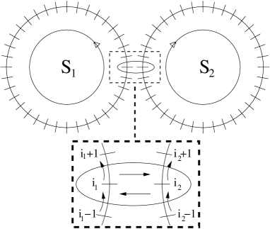
Figure 1: Illustration of two mass transport models with periodic boundary conditions, connected through a contact made of a single additional link. A zoom over the contact is also shown in the dashed frame; arrows indicate the oriented links through which mass is transported.

In order to define the dynamics at the contact, we extend the dynamical rules in such a way that a mass located at site $i_{1}\in\mathcal{S}_{1}$ at the interface (see Fig. 1), is transferred with rate $\varphi_{1}(\mu|m)$ either to the neighboring site $i_{1}+1$ or with the same rate to site $i_{2}\in\mathcal{S}_{2}$. A similar rule is applied for a mass located on site $i_{2}$, regarding the transfer to $i_{1}$. Hence the two homogeneous systems simply combine to an inhomogeneous one, for which one can find a factorized steady-state, as $v(\mu)$ is site-independent, and as the graph on which the system is defined satisfies the required geometrical constraint graph-MTM . It follows that in this case the additivity condition (4), (5) holds, and the ITPs of the two systems equalize.

Let us now give some examples illustrating the consequences of the equalization of ITPs for two systems in contact, within the framework of the above model. It should first be noticed that the equalization of ITPs enforces constraints on the densities of the two systems, which may thus differ one from the other if the two systems have different equations of state. An interesting situation arises in the presence of a condensate. To be more specific, let us consider two different mass transport models, without impurities. The two systems are initially both isolated, and we assume that the first one contains a condensate, while the second one does not. This means that, in this initial stage, $\lambda_{1}=0$ whereas $\lambda_{2}>0$. When put into contact, the dynamics will be such as to equalize the ITPs $\lambda_{1}$ and $\lambda_{2}$, through a transfer of mass between the two systems. As $\lambda$ generically decreases when the density increases, mass has to be transferred from $\mathcal{S}_{1}$ to $\mathcal{S}_{2}$. Withdrawing mass from $\mathcal{S}_{1}$ actually does not affect the fluid phase of $\mathcal{S}_{1}$ (at least in a quasi-static limit) as long as the average density $\rho_{1}$ remains above the critical density $\rho_{1}^{crit}$, and mass is taken from the condensate only, in this first stage. Assuming that the critical density of $\mathcal{S}_{2}$, $\rho_{2}^{crit}$, is infinite, the condensate in $\mathcal{S}_{1}$ eventually disappears, and both ITPs converge to a strictly positive value that lies between the initial values of $\lambda_{1}$ and $\lambda_{2}$. Yet, the final densities of the two systems are different in general.

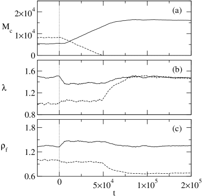
Figure 2: Time dependence of the masses of the condensates (a), the ITPs (b) and the densities of the fluid phases (c) in two mass transport models in contact, $\mathcal{S}_{1}$ (solid line) and $\mathcal{S}_{2}$ (dashed line) –see Fig. 1. Both of them contain an impurity site. Parameter values are $\xi_{1}=1.5$ and $\xi_{2}=1$ for the impurities, $\eta_{1}=2$ and $\eta_{2}=1$ for the homogeneous parts –see text. The systems are separately in steady state (with overall initial densities $\rho_{1}=\rho_{2}=2$) before the contact is established at time t=0 (dotted line). Note that the ITPs eventually equalize, and that the difference between the fluid densities increases after the contact is established.

One may also think of more complex situations. Let us consider the case where each of the two systems contains an impurity (as defined in Sec. III.2.2), with respective parameters $\xi_{1}$ and $\xi_{2}$ ($\xi_{2}<\xi_{1}$). In addition, we consider different functions $f_{\rm hom}(m)$ for the homogeneous part of each system, namely $f_{{\rm hom},\nu}(m)=m^{\eta_{\nu}-1}$ in system $\mathcal{S}_{\nu}$, $\nu=1,2$. Before the contact is switched on, both systems are in steady state and contain a condensate, so that $\lambda_{1}=\xi_{1}$ and $\lambda_{2}=\xi_{2}$. When the contact is established at $t=0$, the ITPs tend to equalize, and as $\lambda_{2}<\lambda_{1}$, mass is transferred from $\mathcal{S}_{2}$ to $\mathcal{S}_{1}$ (as $\rho$ decreases with $\lambda$), independently of the values of $\eta_{1}$ and $\eta_{2}$. But as $\mathcal{S}_{1}$ already contains a condensate, the density of the fluid phase is fixed, and all the mass brought to $\mathcal{S}_{1}$ is actually transferred to the condensate. Hence, the final state corresponds to $\lambda_{1}=\lambda_{2}=\xi_{1}$, with $\mathcal{S}_{1}$ containing a larger condensate than initially, and $\mathcal{S}_{2}$ being at a density $\rho_{2}(\lambda_{2}=\xi_{1})<\rho_{2}^{crit}=\rho_{2}(\lambda_{2}=\xi_{2})$, so that there is no more condensate in $\mathcal{S}_{2}$. Fig. 2 presents the results of numerical simulations of the above situation, showing in particular that the condensate of $\mathcal{S}_{2}$ disappears once the contact is established. In addition, this simulation confirms that the ITPs of the two systems are controlling the direction of the flux of mass. Indeed, mass is transferred from $\mathcal{S}_{2}$ to $\mathcal{S}_{1}$ even though the density of the fluid is larger in $\mathcal{S}_{1}$ than in $\mathcal{S}_{2}$, which might seem rather counterintuitive given that the two systems are in contact through their fluid phases only.

Note also that strictly speaking, the determination of $\lambda$ using the equation of state is valid only in a steady state, so that one should wait until the density $\rho$ is stationary before determining $\lambda$ from $\rho$. Still, for the purpose of illustration, we present here $\lambda(t)$ deduced from the fluid density $\rho_{f}(t)$ even in the nonstationary regime. This is meaningful if the exchanges between the two systems are slow enough so that each system may be considered in a quasi-steady state.

¿From the above result, one sees that the impurity in system $\mathcal{S}_{1}$ (that is, the one with the larger value of $\xi$) plays the role of a reservoir of mass that fixes the value of the ITP of $\mathcal{S}_{2}$ to $\lambda_{2}=\xi_{2}$. Interestingly, $\mathcal{S}_{1}$ only needs to contain a mass of the same order as that of $\mathcal{S}_{2}$ to act as a reservoir, as the ITP $\lambda_{1c}$ of the condensate is independent of its mass $M_{1c}$ as long as $M_{1c}$ is macroscopic. On the contrary, usual reservoirs require a mass much larger than that of the systems they are in contact with.

As we have seen on these simple examples, the notion of ITP allows one to make, essentially without calculations, non-trivial predictions about the behavior of mass transport models put into contact (for instance, the final densities of both systems); only the knowledge of the equation of state for each system taken separately is required. However, such predictions can be made only if the ITPs equalize. In the present case of mass transport models, this equalization holds as long as the transition rates obey the relation (70). What are the conditions for such an equalization to hold in more general situations will be the topic of the next section.

IV.3 Characterization of the dynamics at the contact

In this section, we consider the more general case of two systems in contact as schematically illustrated in Fig. 3. The dimension $d$ of the two systems is arbitrary, and the contact consists in a set of links between the two systems. Generically, the contact relates some parts of the borders of each system, as shown in Fig. 3, but one may also think of more complex types of contact.

Figure 3: Schematic drawing of two generic systems in contact. Arrows illustrate the possibility to transfer a conserved quantity between the two systems. Contrary to Fig. 1, the contact generally extends over many sites.

As mentioned in Sec. IV.1, the dynamics at the contact plays an essential role in the possibility to equalize the ITPs of two connected systems. This equalization occurs if the condition (69), or equivalently, the additivity condition (4), (5), is fulfilled. Yet, testing this condition is a priori very difficult, and its interpretation in terms of the microscopic dynamics at the contact is not obvious. On the other hand, if two systems $\mathcal{S}_{1}$ and $\mathcal{S}_{2}$ are connected and globally isolated, the flux $\phi_{1\to 2}$ transferred from $\mathcal{S}_{1}$ to $\mathcal{S}_{2}$ through the contact has to be equal, in steady state, to the reverse flux $\phi_{2\to 1}$ going from $\mathcal{S}_{2}$ to $\mathcal{S}_{1}$.

For the sake of simplicity, we now introduce some assumptions that allow one to analyze, at least in a simple case, this generic problem of the contact between two systems. For definiteness, let us consider lattice systems $\mathcal{S}_{1}$ and $\mathcal{S}_{2}$ that may exchange a globally conserved quantity. The set of sites belonging to the contact in system $\mathcal{S}_{\nu}$, $\nu=1,2$, is denoted as $\mathcal{C}_{\nu}$. As already mentioned, the situations considered correspond to the weak coupling limit. In the present context, this means that the flux per site crossing the contact is typically much smaller than the local flux between two sites of a given system, so that the contact does not perturb the dynamics of each system, apart from the (slow) exchange of $Q$. In addition, the specific assumptions used in the following arguments are that:

(i) the flux $\phi_{1\to 2}$ depends only on $\lambda_{1}$, and not on the properties of $\mathcal{S}_{2}$ such as $\lambda_{2}$; respectively, $\phi_{2\to 1}$ depends only on $\lambda_{2}$ (yet, the total flux $\phi_{1\to 2}-\phi_{2\to 1}$ depends on both $\lambda_{1}$ and $\lambda_{2}$);

(ii) the probability weights of $\mathcal{S}_{1}$ and $\mathcal{S}_{2}$, each one considered as isolated, are factorized as products of one-site weights.

In the spirit of hypothesis (i), the dynamics at the contact is defined by the probability rate $\varphi_{i_{1}}^{c}(\mu|q_{i_{1}})$ to transfer $\mu$ from site $i_{1}\in\mathcal{C}_{1}$ in $\mathcal{S}_{1}$ to $\mathcal{S}_{2}$; a similar rate $\varphi_{i_{2}}^{c}(\mu|q_{i_{2}})$ defines the transfer from $i_{2}\in\mathcal{C}_{2}$ in $\mathcal{S}_{2}$ to $\mathcal{S}_{1}$. Under these assumptions, one can compute the fluxes $\phi_{1\to 2}(\lambda_{1})$ and $\phi_{2\to 1}(\lambda_{2})$; in particular, $\phi_{1\to 2}(\lambda_{1})$ reads

$$\phi_{1\to 2}(\lambda_{1})=\sum_{i\in\mathcal{C}_{1}}\int_{0}^{\infty}dq_{i}\,P_{1}(q_{i})\int_{0}^{q_{i}}d\mu\,\mu\,\varphi_{i}^{c}(\mu|q_{i}).$$ (71)

where $P_{1}(q_{i})$ is the single site probability distribution in $\mathcal{S}_{1}$. Given that $P_{1}(q)=c_{1}f_{1}(q)\exp(-\lambda_{1}q)$, $c_{1}$ being a normalization constant, it follows that

$$\phi_{1\to 2}(\lambda_{1})=c_{1}\int_{0}^{\infty}dq\int_{0}^{q}d\mu\,\mu\varphi_{1}^{tot}(\mu|q)f_{1}(q)\,e^{-\lambda_{1}q}\;,$$ (72)

where we have introduced the “total” rate

$$\varphi_{1}^{tot}(\mu|q)=\sum_{i\in\mathcal{C}_{1}}\varphi_{i}^{c}(\mu|q)\;.$$ (73)

By exchanging the indexes of the systems, a similar relation holds for $\phi_{2\to 1}(\lambda_{2})$.

For the two systems to equalize their ITPs, it is necessary that the equality $\phi_{1\to 2}(\lambda_{1})=\phi_{2\to 1}(\lambda_{2})$ leads to $\lambda_{1}=\lambda_{2}$, for arbitrary values of (say) $\lambda_{1}$. In other words, the two functions $\phi_{1\to 2}(\lambda)$ and $\phi_{2\to 1}(\lambda)$ must be identical. Let us then compute the difference $\phi_{1\to 2}(\lambda)-\phi_{2\to 1}(\lambda)$. After a straightforward calculation, this difference can be expressed as

$$\phi_{1\to 2}(\lambda)-\phi_{2\to 1}(\lambda)=c_{1}c_{2}\int_{0}^{\infty}dq_{1}\int_{0}^{\infty}dq_{2}\int_{0}^{q_{1}}d\mu$$ (74)

$$\times \mu\,e^{-\lambda(q_{1}+q_{2})}[\varphi_{1}^{tot}(\mu|q_{1})f_{1}(q_{1})f_{2}(q_{2})$$

$$\qquad-\varphi_{2}^{tot}(\mu|q_{2}+\mu)f_{1}(q_{1}-\mu)f_{2}(q_{2}+\mu)]$$

In order that $\phi_{1\to 2}(\lambda)-\phi_{2\to 1}(\lambda)$ vanishes for any value of $\lambda$, it is necessary and sufficient that the expression between brackets vanishes, that is

$$\varphi_{1}^{tot}(\mu|q_{1})f_{1}(q_{1})f_{2}(q_{2})$$ (75)

$$\qquad\qquad=\varphi_{2}^{tot}(\mu|q_{2}+\mu)f_{1}(q_{1}-\mu)f_{2}(q_{2}+\mu)$$

One can check that Eq. (75) is precisely a detailed balance relation between configurations $(q_{1},q_{2})$ and $(q_{1}^{\prime}=q_{1}-\mu,q_{2}^{\prime}=q_{2}+\mu)$. Yet, let us emphasize that this detailed balance relation does not concern the true microscopic dynamics at the contact, but rather an effective, coarse-grained dynamics, defined by $\varphi_{\nu}^{tot}(\mu|q)$ that reduces the contact to a single effective link. To illustrate this point, one can imagine a contact made of two fully biased links between $\mathcal{S}_{1}$ and $\mathcal{S}_{2}$. The first link can only transfer the conserved quantity $Q$ from $\mathcal{S}_{1}$ to $\mathcal{S}_{2}$, whereas the second one only allows $Q$ to be transferred from $\mathcal{S}_{2}$ to $\mathcal{S}_{1}$. Then, the microscopic dynamics at the contact does not satisfy detailed balance, but the coarse-grained dynamics may fulfill this condition.

Note that if the true contact already consists in a single link as illustrated on Fig. 1, the effective dynamics is the true one, so that the dynamics at the contact really satisfies detailed balance. This is basically the interpretation of the condition used in Eq. (70), according to which $v(\mu)$ has to be the same in the two systems: this condition ensures detailed balance at the contact, even though detailed balance breaks down in each system due to the presence of fluxes. In constrast, if the functions $v(\mu)$ were to be different in the two systems the ITPs would not equalize due to the lack of detailed balance at the contact.

In summary, we have seen the importance of the dynamics of the contact, which must fulfill condition (69) to ensure the equalization of the ITPs among the connected systems. On the other hand, the effective detailed balance Eq. (75) is a priori a less general statement, due to the simplifying assumptions used to derive it. However it provides us with a physical interpretation of the conditions required for the dynamics at the contact. One may hope that the resulting physical picture might be relevant beyond the strict validity of Eq. (75).

IV.4 Measure of an ITP

IV.4.1 Notion of ITP-meter

An essential issue about ITPs would be the ability to measure them. In analogy to the measurement of temperature in equilibrium statistical mechanics, one could imagine to realize such a measurement by connecting an auxiliary system to the system under consideration. This problem has also been addressed in Hatano . In this general framework, we shall call this (perhaps conceptual) instrument “ITP-meter”, in reference to the nomenclature “thermometer”. There are three essential requirements which have to be fulfilled to perform such an implementation. First, the values of $\lambda$ in the gauged system and in the ITP-meter need to equalize. Second, the measured system must not be disturbed by the measurement, so that the ITP-meter should be small with respect to the system upon which the measure is performed. Third, the equation of state of the ITP-meter has to be known, since one needs to deduce the value of its ITP from the measure of a directly accessible physical quantity. Accordingly, these different conditions turn the realization of an ITP-meter into a highly nontrivial problem.

Nevertheless it is possible for certain simple cases to realize a measurement with an ITP-meter, using for instance two connected mass transport models as described in Sec. IV.2. The systems are similar to the ones shown in Fig. 1, but now $\mathcal{S}_{2}$, used as an ITP-meter, is much smaller than $\mathcal{S}_{1}$. We present in Fig. 4 numerical simulations in which each system $\mathcal{S}_{\nu}$ ($\nu=1,2$) is homogeneous, and obeys the transport rate defined in Eq. (70) with $f_{\nu}(m)=m^{\eta_{\nu}-1}$, where $\eta_{1}\neq\eta_{2}$. By measuring the density $\rho_{\nu}$ of each system, one can determine the value of $\lambda_{\nu}$ using the equations of state, namely $\lambda_{\nu}=\eta_{\nu}/\rho_{\nu}$. In practice, one would of course only measure the density of the ITP-meter, but here we determine both $\lambda_{1}$ and $\lambda_{2}$ to check the validity of the approach.

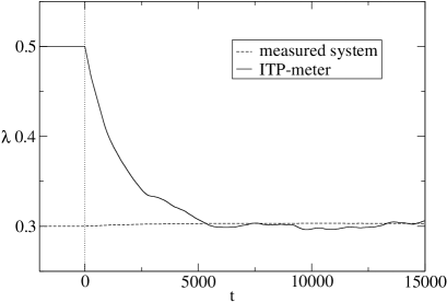
Figure 4: Measurement process on a system $\mathcal{S}_{1}$ using an ITP-meter $\mathcal{S}_{2}$. The values of the ITPs $\lambda_{1}$ (dashed line) and $\lambda_{2}$ (solid line) are plotted versus time. The systems are characterized by parameters $\eta_{1}=3$, $\eta_{2}=5$ (see text). The contact is switched on at time $t=0$. Initially, $\rho_{1}=\rho_{2}=10$, so that $\lambda_{1}=0.3$ and $\lambda_{2}=0.5$. Note that $\lambda_{1}$ almost stays constant whereas after a sufficient time $\lambda_{2}$ converges to $\lambda_{1}$.

Numerical simulations are run using systems of size $N_{1}=64510$ and $N_{2}=1024$, with equal initial densities, $\rho_{1}=\rho_{2}=\rho$, and with $\eta_{1}<\eta_{2}$. Hence the initial values of the ITPs are different, namely $\lambda_{1}=\eta_{1}/\rho$ and $\lambda_{2}=\eta_{2}/\rho$. At time zero the contact between the two systems is switched on, and mass flows from $\mathcal{S}_{1}$ to the ITP-meter $\mathcal{S}_{2}$, since $\lambda_{1}<\lambda_{2}$. As predicted theoretically and confirmed by the numerical simulations, the ITPs of the two systems equalize once the steady-state is reached. In addition, the value of $\lambda_{1}$ does not change significantly along this process, which is the basic requirement for a non-perturbative measurement. Accordingly, the ITP-meter indeed measures the value of $\lambda_{1}$. Quite importantly, this measure is done without knowing the value of the parameter $\eta_{1}$ defining the dynamics of $\mathcal{S}_{1}$. This value was only used to determine $\lambda_{1}$ from $\rho_{1}$ in order to check the measurement.

The above example illustrates on a simple model that it is in principle possible to measure an ITP using an ITP-meter in nonequilibrium systems. Still, in more realistic situations, finding a suitable definition for the dynamics at the contact that allows for the equalization of ITPs turns out to be a major challenge. As seen in the preceding section, Eq. (75) gives a condition for the equalization of ITPs between the two systems, and it provides useful information to design the contact. Yet, it is important to notice that Eq. (75) is a detailed balance relation with respect to the stationary distributions of $\mathcal{S}_{1}$ and $\mathcal{S}_{2}$. Hence, to satisfy this relation, one requires some important information on the gauged system, namely its steady state weight $f_{1}(q)$. Such an information is usually unavailable in nonequilibrium systems, contrary to what happens in equilibrium, where the weights are either uniform (microcanonical ensemble) or given by the Boltzmann-Gibbs factor (canonical ensemble).

IV.4.2 Measure within subsystems

An alternative route, that has been exploited recently in the context of granular matter Nowak ; Swinney , consists in trying to determine the ITP through an interpretation of direct measurements on the system, instead of using an auxiliary system (the ITP-meter) . More precisely, let us consider a system with a globally conserved quantity $Q$. Then, from Eq. (II.2), the variance of the quantity $Q_{N}$, measured over a “mesoscopic” subsystem of size $N$, obeys the following relation, derived from the grand-canonical ensemble:

$$\langle Q_{N}^{2}\rangle-\langle Q_{N}\rangle^{2}=-\frac{d\langle Q_{N}\rangle}{d\lambda}\;.$$ (76)

Let us assume, consistently with the additivity condition (4), (5), that the variance of $Q_{N}$ is linear in the subsystem size $N$, at least for $1\ll N\ll N_{\rm tot}$, where $N_{\rm tot}$ is the size of the global system. Hence the variance may be written as

$$\langle Q_{N}^{2}\rangle-\langle Q_{N}\rangle^{2}=Ng(\rho)$$ (77)

with $\rho=\langle Q_{N}\rangle/N$. Then Eq. (76) leads to

$$g(\rho)=-\frac{d\rho}{d\lambda}\;.$$ (78)

Given a reference point $(\rho_{0},\lambda_{0})$, one can then determine the equation of state of the system, simply by integrating Eq. (78) numerically:

$$\lambda=\int_{\rho}^{\rho_{0}}\frac{d\rho}{g(\rho)}+\lambda_{0}\;.$$ (79)

As a first example, we now apply this procedure to a mass transport model on a ring with dynamics defined by $f(m)=(1+m)^{2}$ and $v(\mu)=1$ (see Eq. (28)), for which the equation of state $\lambda(\rho)$ cannot be determined easily by scaling arguments as in Sec. II.4. By measuring in a numerical simulation the variance of the mass $M_{N}$ over subsystems of different size $N$, we find as expected a linear behavior in $N$ already for small sizes (see inset of Fig. 5(a)), since the grand-canonical distribution is fully factorized. The result of the numerical integration for the equation of state is in very good agreement with the theoretical curve obtained using the grand-canonical ensemble (see Fig. 5(a)), for which $\rho$ can be determined as a function of $\lambda$, as done for instance in Eq. (47).

The fact that this procedure works as well for cases in which the steady state does not fully factorize, can be seen in another numerical experiment exhibiting a pair-factorized steady state. Let the dynamics be defined as in Eq. (34), with $v(\mu)=1$ and $g(m,n)=m+n$, that is, we assume $\alpha=1$, $\beta=0$ and $\gamma=1$ in Eq. (36). Measuring again the variance of the mass $M_{N}$ over subsystems of size $N$, shows that the measurement of the ITP $\lambda$ should be performed for higher values of $N$ than in the fully factorized case to have access to the linear regime (see inset of Fig. 5(b)). Note that the results of the measurement (see Fig. 5(b)) agree equally well with the theoretical curve, which can be obtained in this case by the simple scaling argument presented in Sec. II.4.2.

In these examples, we obtained for simplicity a reference point ($\rho_{0},\lambda_{0}$) using the theoretical equation of state. In a more realistic situation where the equation of state is unknown, one can estimate as well a reference point only through the information obtained from the measured variances. Measuring numerically the function $g(\rho)$ for large values of $\rho$, one can fit its asymptotic (large $\rho$) expression with a power law, $g(\rho)\approx A\rho^{\delta}$; in the two models above, one has $\delta=2$. Then, assuming that $\lambda$ vanishes when $\rho\to\infty$, and that $\delta>1$, the reference value $\lambda_{0}$ corresponding to a given large density $\rho_{0}$ is obtained as

$$\lambda_{0}=\int_{\rho_{0}}^{\infty}\frac{d\rho}{g(\rho)}\approx\int_{\rho_{0}}^{\infty}\frac{d\rho}{A\rho^{\delta}}=\frac{1}{A(\delta-1)\rho_{0}^{\delta-1}}\;.$$ (80)

Note that alternatively, one may also determine a reference point from the distribution of $Q_{N}$, as proposed in Dauchot .

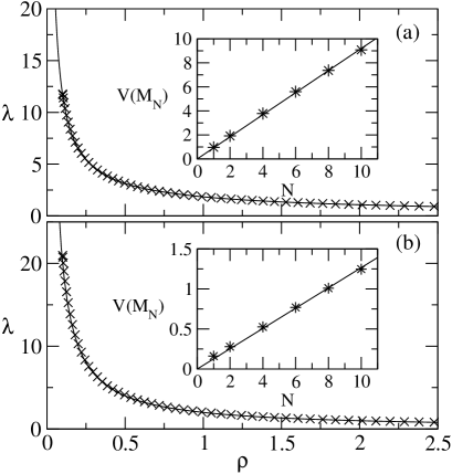
Figure 5: Equation of state $\lambda$ as a function of $\rho$ in two mass transport models, obtained by numerical simulations using the measurement procedure described in the text ($\times$), compared with the theoretical prediction $\rho(\lambda)$ derived in the grand-canonical ensemble (solid line); (a) fully factorized steady state with $f(m)=(1+m)^{2}$, (b) pair-factorized case with $g(m,n)=m+n$. Insets: dependence of the variance $V(M_{N})$ on the subsystem size $N$ ($\ast$) for densities $\rho=1.2$ (a) and $\rho=0.5$ (b); solid lines are linear fits.

Accordingly, the present approach provides a rather simple way to measure experimentally or numerically ITPs in realistic systems for which no information on the microscopic probability distribution (like the weight factors $f(m)$ for instance) is available. As mentioned above, this method has already been used in the context of granular material Nowak ; Swinney . However, it was thought to rely on Edwards’ thermodynamic construction which explicitely assumes the equiprobability of states compatible with the constraints (conserved quantities), whereas this assumption is not necessary, as illustrated in the above examples –see also Dauchot . Indeed, the validity of the approach is much more general, making it a convenient way to determine practically ITPs in nonequilibrium systems.

V Conclusions

In this paper, we highlight that the notion of generalized ITPs for steady-state nonequilibrium systems serves as a new tool in the study of nonequilibrium phenomena. Within the range of validity of the additivity condition (4), (5), there is a vast variety of models for which our approach can be useful, like models with a factorized steady-state distribution, or one-dimensional systems described by a matrix product ansatz or the transfer matrix method (at least with finite matrices). The method should also be of interest for models which are well approximated by a mean field approach.

Introduced by generalizing the equilibrium concept, for which physical intuition is well developed, ITPs benefit from a rather clear physical interpretation. They provide a convenient way to describe the coexistence of two phases, as may be easily illustrated on the case of the condensation transition. An essential issue, which made the success of the ITP concept in equilibrium, is the possibility to equalize ITPs in different systems put into contact. Contrary to equilibrium situations, such an equalization is not automatically fulfilled in the nonequilibrium case, and the dynamics at the contact turns out to play a major role. We have derived, under simplifying assumptions, a coarse-grained detailed balance relation that needs to be satisfied by the contact dynamics in order that ITPs equalize. Deriving a more general criterion by relaxing some of the assumptions made would be interesting to gain further insights on this important issue.

A related difficulty with the approach is that the additivity property (4), (5) may be hard to test directly. Still, measuring the variance of the globally conserved quantity over subsystems of a homogeneous system may lead to an indirect test of this property: indeed, one expects that the variance introduced in Eq. (76), becomes linear in $N$ for $N\gg 1$ if the additivity property is satisfied.

¿From the point of view of measurements, it turns out that realizing an ITP-meter remains a major challenge, mostly due to the difficulties with the choice of the dynamics at the contact. Indeed, one would need to find a dynamics for the contact that satisfies the condition for equalization of ITPs (that is, the coarse-grained detailed balance relation (75) or a generalization of it), without having information on the probability weights of the system on which the measure should be done. Alternatively, measurements of ITPs using the variance of the globally conserved quantity in subsystems of “mesoscopic” size seem to be a promising route.

Appendix A Independence of the choice of subsystems

In this appendix, we show that, according to the claim made in Sec. II.1, the value of the ITP $\lambda_{k}$ does not depend on the partition chosen. To this aim, let us relate the ITP $\lambda_{k}$ obtained from the subsystems, to a global ITP defined on the whole system. Knowing that

$$\int\prod_{k=1}^{\ell}dQ_{ka}\;\Psi(\{Q_{ka}\}|\{Q_{k}\})=1$$ (81)

and neglecting the correction term $\epsilon_{N}$ appearing in Eq. (5) in the large N limit, one can derive an expression for $Z(\{Q_{k}\})$ depending on the partition functions of the subsystems

$$Z(\{Q_{k}\})=\int\prod_{k=1}^{\ell}dQ_{ka}\;Z_{a}(\{Q_{ka}\})Z_{b}(\{Q_{k}-Q_{ka}\})\;.$$ (82)

Consistently with the additivity property (4), (5), we assume a general scaling form for the partition functions $Z_{\nu}$ for a large number of sites $N_{\nu}$

$$Z_{\nu}(\{Q_{k\nu}\})=A_{\nu}\exp\left\{N_{\nu}\zeta_{\nu}\left(\frac{Q_{1\nu}}{N_{\nu}},\ldots,\frac{Q_{\ell\nu}}{N_{\nu}}\right)\right\}$$ (83)

This amounts to assuming that $\ln Z_{\nu}(\{Q_{k\nu}\})$ is extensive. This choice allows us to perform a saddlepoint approximation for the integrals in Eq. (82) and thus we obtain

$$Z(\{Q_{k}\}) = N^{\ell}Z_{a}(\{Q^{*}_{ka}\})Z_{b}(\{Q_{k}-Q^{*}_{ka}\})\times$$ (84)

$$\int_{0}^{q_{k}}\prod_{k=1}^{\ell}dq_{ka}\;e^{-N(f_{a}(q_{ka})+f_{b}(q_{ka}))}$$

where $q_{k}=Q_{k}/N$, $q_{k\nu}=Q_{k\nu}/N$ and $q_{k\nu}^{*}=Q_{k\nu}^{*}/N$, $\nu\in\{a,b\}$. The functions $f_{\nu}$ read with $n_{\nu}=N_{\nu}/N$

$$f_{a}(\{q_{ka}\}) = -\frac{n_{a}}{2}\sum_{i,j=1}^{\ell}\frac{\partial^{2}\zeta_{a}}{\partial q_{ia}\partial q_{ja}}\left(\left\{\frac{q_{ka}}{n_{a}}\right\}\right)\Big{|}_{(q_{ia}^{*},q_{ja}^{*})}\times$$

$$\qquad(q_{ia}-q_{ia}^{*})(q_{ja}-q_{ja}^{*})$$

$$f_{b}(\{q_{ka}\}) = -\frac{n_{b}}{2}\sum_{i,j=1}^{\ell}\frac{\partial^{2}\zeta_{b}}{\partial q_{ia}\partial q_{ja}}\left(\left\{\frac{q_{k}-q_{ka}}{n_{b}}\right\}\right)\Big{|}_{(q_{ia}^{*},q_{ja}^{*})}\times$$ (85)

$$\qquad(q_{ia}-q_{ia}^{*})(q_{ja}-q_{ja}^{*})$$

Taking the logarithm of the above expression, Eq. (84), leads to

$$\ln Z(\{Q_{k}\}) = \ln Z_{a}(\{Q_{ka}^{*}\})+\ln Z_{b}(\{Q_{k}-Q_{ka}^{*}\})$$ (86)

$$+ \ln\xi(q_{k})$$

where $\xi(q_{k})$ is given by the finite integrals of Eq. (84). We thus obtain for the derivative with respect to $Q_{k}$, using Eq. (9),

$$\frac{\partial\ln Z(\{Q_{k}\})}{\partial Q_{k}}=\lambda_{k}\frac{\partial Q_{ka}^{*}}{\partial Q_{k}}+\lambda_{k}\left(1-\frac{\partial Q_{ka}^{*}}{\partial Q_{k}}\right)+\frac{1}{N}\frac{\partial\ln\xi}{\partial q_{k}}\;.$$ (87)

Since $\xi(q_{k})$ is expected to be bounded when $N\to\infty$ while the ratio $q_{k}=Q_{k}/N$ is kept constant, the last term vanishes in the thermodynamic limit, and we find

$$\frac{\partial\ln Z(\{Q_{k}\})}{\partial Q_{k}}=\lambda_{k}$$ (88)

where the value of $\lambda_{k}$ stays finite in the limit defined above due to the scaling form of $Z_{\nu}$ in Eq. (83). The fact that we can compute the value of $\lambda_{k}$ directly from the whole system shows the independence of the partition chosen. This means that the ITPs $\lambda_{k}$ ($k=1,\dots,\ell$) are global values that can be used to characterize the macroscopic state of the whole system.

Appendix B Additivity condition for matrix product ansatz

The aim of this appendix is to show that, under reasonable assumptions, a system described by a matrix product ansatz with finite matrices fulfills the additivity property (4), (5). For the sake of simplicity, we only deal with the case of a single conserved quantity, but generalizations to several conserved quantities are rather straightforward. We also use periodic boundary conditions, though calculations with open boundaries would essentially be similar. Considering a generic lattice model as defined in Eq. (18), the conditional distribution $\Psi(Q_{a}|Q)$ reads:

$$\Psi(Q_{a}|Q)=\frac{1}{Z(Q)}\,\mathrm{Tr}[R_{a}(Q_{a})R_{b}(Q-Q_{a})]$$ (89)

To proceed further, one needs to introduce the Laplace transforms $\hat{R}(s)$ and $\hat{M}(s)$ of $R(Q)$ and $M(q)$ respectively, which leads to $\hat{R}(s)=\hat{M}(s)^{N}$. Making the further hypothesis that $\hat{M}(s)$ is invertible, one can find a matrix $B(s)$ such that $\hat{M}(s)=\exp[B(s)]$, yielding $\hat{R}(s)=\exp[NB(s)]$. The matrix $B(s)$ can be decomposed into a sum of two complex-valued matrices Horn :

$$B(s)=D(s)+L(s)$$ (90)

where $D(s)$ is a diagonalizable matrix, and $L(s)$ is a nilpotent one, meaning that there exists a positive integer $p(s)$ such that $L(s)^{p(s)}=0$. In addition, the matrices $D(s)$ and $L(s)$ commute. Using Eq. (90), one has

$$\hat{R}(s)=e^{ND(s)}\,e^{NL(s)}\\ =e^{ND(s)}\,{\cal P}_{s}(NL(s))$$ (91)

where ${\cal P}_{s}$ is a polynomial of degree $p(s)-1$, since higher order terms in the expansion of $\exp[NL(s)]$ vanish. Accordingly, in the large $N$ limit, the dominant contribution to $\hat{R}(s)$ is proportional to $N^{p(s)-1}\exp[ND(s)]$. Then, as $D(s)$ is diagonalizable, there exists a matrix $V(s)$ such that $D(s)=V^{-1}(s)\Lambda(s)V(s)$, where $\Lambda(s)$ is the diagonal matrix. It results that

$$e^{ND(s)}=V^{-1}(s)\,e^{N\Lambda(s)}V(s)$$ (92)

so that the dominant contribution to $\exp[ND(s)]$ is proportional to $\exp[N\ell_{1}(s)]$, $\ell_{1}(s)$ being the eigenvalue of $D(s)$ with the largest real part. Altogether, $\hat{R}(s)$ takes the following form, to leading order in $N$:

$$\hat{R}(s)\sim N^{p(s)-1}\exp(N\ell_{1}(s))K(s)$$ (93)

where $K(s)$ is a matrix that does not depend on $N$. Then $R(Q)$ is obtained through an inverse Laplace transform:

$$R(Q)\sim\int_{s_{0}-i\infty}^{s_{0}+i\infty}\frac{ds}{2\pi i}\,N^{p(s)-1}\exp[N(\ell_{1}(s)+s\rho)]K(s)$$ (94)

with $\rho=Q/N$, and where $s_{0}$ is an arbitrary real number, greater than the real part of all the singularities of the integrand. Assuming that the equation $G(s)=d\ell_{1}/ds+\rho=0$ has a solution $s^{*}$, and that $s_{0}$ can be chosen as $s^{*}$, a saddle-point calculation shows that the dominant contribution to $R(Q)$ is proportional to $\exp[N(\ell_{1}(s^{*})+s^{*}\rho)]$. The remaining Gaussian integral around the saddle (on the imaginary axis) converges since $G^{\prime\prime}(s)=\ell_{1}^{\prime\prime}(s)>0$. This last property can be shown in the following way. The logarithm of the grand-canonical partition function satisfies $\ln\tilde{Z}(s)\approx N\ell_{1}(s)$, with the identification $\lambda=s$. Then, from Eq. (II.2), the second derivative of $\ln\tilde{Z}$ is the variance of $Q$, which is positive; hence $\ell_{1}^{\prime\prime}(s)>0$. Since $Z(Q)=\mathrm{Tr}R(Q)$, $Z(Q)$ is also proportional to $\exp[N(\ell_{1}(s^{*})+s^{*}\rho)]$. As a result, one finds

$$\ln\mathrm{Tr}[R_{a}(Q_{a})R_{b}(Q_{b})] \approx N_{a}(\ell_{1}^{a}(s_{a}^{*})+s_{a}^{*}\rho_{a})$$

$$\qquad\qquad+N_{b}(\ell_{1}^{b}(s_{b}^{*})+s_{b}^{*}\rho_{b})$$

$$\approx \ln Z_{a}(Q_{a})+\ln Z_{b}(Q_{b})\;,$$

from which the additivity condition (4), (5) follows.

Appendix C Pair factorized steady state for a continuous mass model

Let us show that the model introduced in Sec. II.4.2, defined through the transport rate given in Eq. (34), leads to a pair factorized steady state (35). This can be verified with the master equation for this model, which reads:

$$\frac{dP(\{m_{i}\},t)}{dt} = \sum_{i=1}^{N}\int_{0}^{m_{i+1}}d\mu\,\varphi(\mu|m_{i-1},m_{i}+\mu,m_{i+1}-\mu)P(\ldots m_{i}+\mu,m_{i+1}-\mu,\ldots,t)$$ (96)

$$- \sum_{i=1}^{N}\int_{0}^{\infty}d\mu\,\varphi(\mu|m_{i-1},m_{i},m_{i+1})P(\{m_{i}\},t)\;$$

where $P(\{m_{i}\},t)$ describes the time evolution of the probability of a microstate $\{m_{i}\}$. In the steady state the time derivative vanishes. Plugging Eqs. (34) and (35) into the master equation and dividing by $Z^{-1}\prod_{i=1}^{N}g(m_{i},m_{i+1})$ yields:

$$\sum_{i=1}^{N}\int_{0}^{m_{i+1}}d\mu\,v(\mu)\frac{g(m_{i},m_{i+1}-\mu)}{g(m_{i},m_{i+1})}\frac{g(m_{i+1}-\mu,m_{i+2})}{g(m_{i+1},m_{i+2})}$$ (97)

$$= \sum_{i=1}^{N}\int_{0}^{\infty}d\mu\,v(\mu)\frac{g(m_{i-1},m_{i}-\mu)}{g(m_{i-1},m_{i})}\frac{g(m_{i}-\mu,m_{i+1})}{g(m_{i},m_{i+1})}$$

Substituting $i+1$ by $i$ on the left hand side and knowing that $g(m,n)=0$ for values of $m$ or $n$ smaller than zero one finds the above equality verified.

References

- (1) S. de Groot and P. Mazur, Non-equilibrium Thermodynamics, (North-Holland, Amsterdam, 1962).
- (2) J. Casas-Vázquez and D. Jou, Rep. Prog. Phys. 66, 1937 (2003).
- (3) A. Puglisi, A. Baldassarri, and V. Loreto, Phys. Rev. E 66, 061305 (2002); A. Barrat, V. Loreto, and A. Puglisi, Physica A 334, 513 (2004).
- (4) B. N. Miller and P. M. Larson, Phys. Rev. A 20, 1717 (1979); F. Sastre, I. Dornic, and H. Chaté, Phys. Rev. Lett. 91, 267205 (2003).
- (5) T. Hatano and D. Jou, Phys. Rev. E 67, 026121 (2003).
- (6) E. Bertin, O. Dauchot, and M. Droz, Phys. Rev. Lett. 93, 230601 (2004); Phys. Rev. E 71, 046140 (2005).
- (7) M. Criado-Sancho, D. Jou and J. Casas-Vázquez, Phys. Lett. A 350, 339 (2006).
- (8) L. F. Cugliandolo, J. Kurchan, and L. Peliti, Phys. Rev. E 55, 3898 (1997).
- (9) J. Kurchan, J. Phys.: Cond. Matt. 12, 6611 (2000); Nature 433, 222 (2005).
- (10) A. Crisanti and F. Ritort, J. Phys. A. 36, R181 (2003).
- (11) A. Garriga and F. Ritort, Phys. Rev. E 72, 031505 (2005); F. Ritort, J. Phys. Chem. B 109, 6787 (2005).
- (12) M. R. Evans and T. Hanney, J. Phys. A 38, R195 (2005).
- (13) P. F. Arndt, T. Heinzel, and V. Rittenberg, J. Stat. Phys. 97, 1 (1999).
- (14) E. Bertin, O. Dauchot, and M. Droz, Phys. Rev. Lett. 96, 120601 (2006).
- (15) M. R. Evans, S. N. Majumdar and R. K. P. Zia, J. Phys. A 37, L275 (2004).
- (16) S. N. Majumdar, M. R. Evans, and R. K. P. Zia, Phys. Rev. Lett. 94, 180601 (2005).
- (17) M. R. Evans, T. Hanney and S. N. Majumdar, Phys. Rev. Lett. 97, 010602 (2006).
- (18) See e.g. P. Fulde, Electron Correlations in Molecules and Solids, Springer Verlag (1995).
- (19) M. Schröter, D. I. Goldman, H. L. Swinney, Phys. Rev. E 71, 030301(R) (2005).
- (20) B. Derrida, M. R. Evans, V. Hakim, and V. Pasquier, J. Phys. A 26, 1493 (1993).
- (21) F. H. L. Essler and V. Rittenberg, J. Phys. A 29, 3375 (1996); K. Mallick and S. Sandow, J. Phys. A 30, 4513 (1997).
- (22) S. Grosskinski, G. M. Schütz, and H. Spohn, J. Stat. Phys. 113, 389 (2003).
- (23) C. Godrèche, J. Phys. A 36, 6313 (2003).
- (24) T. Hanney and M. R. Evans, Phys. Rev. E 69, 016107 (2004); S. Grosskinski and T. Hanney, Phys. Rev. E 72, 016129 (2005).
- (25) M. R. Evans, S. N Majumdar, and R. K. P. Zia, J. Phys. A 39, 4859 (2006).
- (26) E. R. Nowak, J. B. Knight, E. Ben-Naim, H. M. Jaeger, and S. R. Nagel, Phys. Rev. E 57, 1971 (1998).
- (27) F. Lechenault, F. da Cruz, O. Dauchot, and E. Bertin, J. Stat. Mech. P07009 (2006).
- (28) See e.g., A. Horn and C. R. Johnson, Matrix analysis, Cambridge University Press (1991).