Reading-out the state of a flux qubit by Josephson transmission line solitons

Abstract

We describe the read-out process of the state of a Josephson flux qubit via solitons in Josephson transmission lines (JTL) as they are in use in the standard rapid single flux quantum (RSFQ) technology. We consider the situation where the information about the state of the qubit is stored in the time delay of the soliton. We analyze dissipative underdamped JTLs, take into account their jitter, and provide estimates of the measuring time and efficiency of the measurement for relevant experimental parameters.

I Introduction

The last few years have brought substantial breakthroughs in experiments with Josephson qubits, with further progress depending to a large extent on our ability to control the circuits with high precision and, at the same time, avoid decoherence. One of the promising ideas combines Josephson flux qubits with the well developed classical rapid single flux quantum (RSFQ) technology Averin ; Kaplunenko . RSFQ elements should allow for more reliable on-chip control and measurements than what can be achieved with control pulses sent over long coaxial cables. However, they have the drawback to be dissipative and thus noisy. The effect of this noise needs to be investigated, and ways need to be found to minimize it.

In this article we consider one of the possible elements of an RSFQ circuit, namely a Josephson transmission line (JTL). The JTL supports propagating signals in the form of Josephson solitons (phase slips), also called fluxons. As suggested by Averin et al. Averin ballistic fluxons in the JTL can be used to read out the state of a superconducting flux qubit in a setup as shown in Fig. 1. In the proposed schemes the information about the state of a qubit is contained either in the fluxon transmission probability (transmission detection mode) or propagation time (delay time detection mode). Under certain ideal conditions the measurement time is equal to the back-action dephasing time, which proves that the JTL can operate as an ideal detector. In this paper we investigate the efficiency that can be achieved in the delay time detection mode. For that purpose we evaluate the delay time in three different setups: a) when the qubit is kept away from the symmetry point all the time; b) when the qubit is initially prepared at the symmetry point, but the approaching soliton pushes the qubit far from the symmetry point; c) when the qubit is near the symmetry point all the time. We analyze the relation between the delay time and the dissipation as well as the probability of errors introduced by the measurement. Finally, we compare the delay time with the characteristic time uncertainty due to jitter (thermal fluctuations) in the JTL, and we determine how many solitons are needed for a reliable measurement.

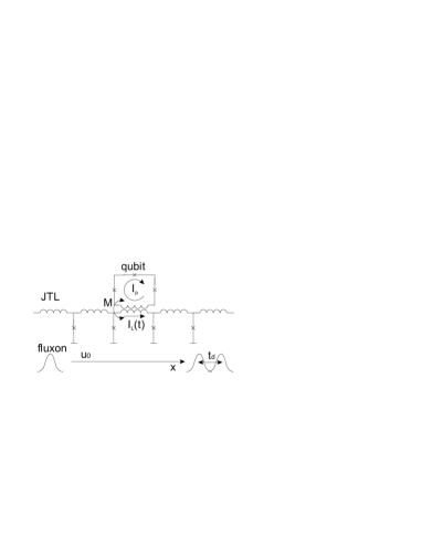
Figure 1: Setup for the read-out of the persistent current qubit based on the delay time of a soliton in the Josephson transmission line (JTL).

For a flux qubit operated far from the symmetry point the eigenstates are persistent current states. The persistent current in the qubit loop induces an external magnetic flux in the JTL, which provides a scattering potential for the fluxon and is responsible for the time delay of the fluxon propagation. The sign of the magnetic flux and the value of the delay time depend on the state of the qubit, which allows measuring its quantum state.

For a qubit prepared in one of the energy eigenstates at the symmetry point the expectation value of the current in the loop vanishes. However, for strong qubit-JTL coupling the fluxon shifts the working point of the qubit away from the symmetry point, and then again the qubit produces a magnetic flux in the JTL. The delay time is approximately the same as if the qubit would have been in a persistent current state corresponding to the induced shift.

For weak qubit-JTL coupling a fluxon shifts the working point of the qubit only slightly around the symmetry point. For this case we demonstrate that the qubit introduces an effective inductance to the JTL with sign depending on the qubit eigenstate. The local change of the inductance of the JTL also serves as a scattering potential for the fluxons, leading to a delay in the fluxon propagation time. This property can in principal be used for a measurement of the qubit at the symmetry point even for weak qubit-JTL coupling.

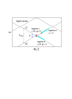
Figure 2: Energy diagram of the qubit for the considered measurement schemes: a) The qubit is kept away from the symmetry point. b) The qubit is initially prepared at the symmetry point, but the approaching soliton pushes the qubit far from the symmetry point. c) The qubit remains near the symmetry point all the time.

For a realistic assessment of the feasibility for the proposed measurement schemes we need to consider the major sources of errors. One of them is thermal noise in the JTL, as a result of which fluxons show fluctuations in their velocity, which lead to an uncertainty (jitter) in the propagation time. In order to distinguish different eigenstates of the qubit the induced delay time should exceed this time jitter. Another source of errors are non-adiabatic transitions of the qubit caused by the moving fluxons. This back-action effect of the JTL on the qubit needs to be taken into account if the qubit is measured at the symmetry point. Still another source of errors are intrinsic relaxation processes of the qubit due to noise not related to the JTL. The relaxation destroys the state of the qubit to be measured and should be much slower than the measurement time. Finally, in order to be detectable the delay times should exceed the time resolution of the RSFQ detector used for delay time measurement.

Our calculations show that for suitable JTL parameters the induced delay times well exceed the time resolution of the RSFQ detector. For strong qubit-JTL coupling the qubit measurement by a single fluxon at the symmetry point, as well as far from it, can be performed with an accuracy of $70-90\%$ for experimentally accessible parameters. For high velocities of the fluxon the measurement efficiency is mostly limited by the jitter and, if the qubit is at the symmetry point, by Landau-Zener transitions. For low velocities the intrinsic relaxation of the qubit may be important. To improve the accuracy one has to use many fluxons for the measurement. If one optimizes the fluxon velocity and number the qubit can be measured with accuracy reaching $99\%$ far from the symmetry point and above $90\%$ at the symmetry point for strong qubit-JTL coupling. The measurement time remains approximately 4 ns for both cases. For weak qubit-JTL couping the qubit prepared at the symmetry point stays there during the whole measurement. In this case the measurement of the qubit is not feasible for standard JTL parameters.

II The model

We focus on the readout of a persistent current qubit PCQ1 ; PCQ2 via its coupling to solitons in a Josephson transmission line (JTL) in a setup as shown in Fig. 1. The qubit consists of a superconducting loop with three Josephson junctions and is inductively coupled to the JTL. The Hamiltonian of the total system is

$$H=H_{qb}+H_{JTL}+H_{I},$$ (1)

where $H_{qb}$ describes the qubit, $H_{JTL}$ the JTL, and $H_{I}$ the qubit-JTL coupling.

In the basis of the two lowest persistent current states, $|0\rangle$, $|1\rangle$, corresponding to currents $\pm I_{p}$ circulating in the qubit loop in opposite directions, the qubit Hamiltonian can be expressed in terms of Pauli matrices PCQ2 ,

$$H_{qb}=-\frac{\epsilon_{0}}{2}\sigma_{z}-\frac{\Delta}{2}\sigma_{x}.$$ (2)

The tunneling amplitude $\Delta$, leading to transitions between both states, is fixed by the experimental setup. The energy bias $\epsilon_{0}$ between the two persistent current states depends on the deviation of the external magnetic flux $\Phi$ in the loop from the symmetry point,

$$\epsilon_{0}=2I_{p}(\Phi-\Phi_{0}/2),$$ (3)

where $\Phi_{0}$ is the magnetic flux quantum.

The Hamiltonian of the discrete dissipationless JTL, shown in Fig. 3, in vanishing external magnetic field can be expressed in terms of the charges $q_{n}$ and the phase differences $\phi_{n}$ of the $n^{\rm th}$ Josephson junctions

$$H_{JTL} = \sum_{n=1}^{N}\left(\frac{q_{n}^{2}}{2C}+E_{J}(1-\cos\phi_{n})\right.$$ (4)

$$+\left.\left(\frac{\Phi_{0}}{2\pi}\right)^{2}\frac{(\phi_{n+1}-\phi_{n})^{2}}{2L}-\frac{\hbar I_{e}}{2e}\phi\right).$$

Here, $N$ is the total number of junctions in the JTL, which here are assumed to be equal, $C$ is the capacitance, and $E_{J}=\hbar I_{c}/2e$ the Josephson energy of the junction with $I_{c}$ being the junction critical current. The inductance of each cell of the JTL is denoted by $L$, and $I_{e}$ is the bias current supplied externally to each junction.

The dimensions of the qubit are much smaller than the length $a$ of a unit cell of the JTL. Therefore, one can assume that the qubit is inductively connected only to one cell of the JTL denoted by label $m$. The corresponding mutual inductance is $M=k\sqrt{L_{qb}L}$, where $L_{qb}$ is the inductance of the qubit loop and $k$ is the coefficient of coupling. Thus the Hamiltonian of the qubit-JTL interaction in the linear response regime is given by

$$H_{I}=\sigma_{z}MI_{p}I_{L}=-\frac{g}{2}\sigma_{z}(\phi_{m}-\phi_{m+1}),$$ (5)

where $I_{L}$ is the electrical current in the inductance of the $m$-th JTL cell and $g=2I_{p}M\Phi_{0}/(2\pi L)$ is the effective qubit-JTL coupling strength.

The classical dynamics of the uniform, discrete, dissipative JTL is governed by Kirchhoff circuit equations Likharev which lead to a system of $N$ discrete sine-Gordon equations

$$\frac{\ddot{\phi}_{n}}{\omega_{p}^{2}}+\frac{\dot{\phi}_{n}}{\omega_{c}}+\sin\phi_{n} = \frac{I_{e}}{I_{c}}+\frac{1}{L}(\Phi^{e}_{n-1}-\Phi^{e}_{n})$$

$$-\frac{\Phi_{0}}{2\pi LI_{c}}\left(\phi_{n-1}-2\phi_{n}+\phi_{n+1}\right).$$

Here, $\omega_{p}=(2eI_{c}/\hbar C)^{1/2}$ is the plasma frequency of the junction, $\omega_{c}=2eI_{c}/\hbar G_{N}$ the junction characteristic frequency with $G_{N}$ being the normal conductance of the junction determining the dissipation in the system, and $\Phi^{e}_{n}$ is the external magnetic flux in the $n-$th cell induced by the qubit.

For low inductances, $LI_{c}\ll\Phi_{0}$, and weak external magnetic fields, $\Phi_{n}^{e}\ll\Phi_{0}$, the phases $\phi_{n}$ of the neighboring junctions are close to each other, and we can rewrite (II) in dimensionless differential form,

$$\ddot{\phi}-\phi_{xx}+\sin\phi=j_{e}-\alpha\dot{\phi}+f^{qb}(\phi,x).$$ (7)

Here the time $t$ and continuous space variable $x$ are measured in the units of the inverse plasma frequency $\omega_{p}^{-1}$ and the Josephson penetration depth $\lambda_{J}=a\left(\Phi_{0}/(2\pi LI_{c})\right)^{1/2}$, respectively, and the phase difference $\phi(x)$ is a function of $x$. Furthermore, $\alpha=\omega_{p}/\omega_{c}$ is the dissipation strength due to a non-vanishing normal conductance $G_{N}$, and $f^{qb}(\phi,x)$ is the perturbation induced by the qubit.

In the following sections we will show that far from the symmetry point, $\epsilon_{0}\gg\Delta$, the perturbation is created by the magnetic flux due to the qubit and can be expressed as

$$f^{qb}_{\rm flux}(\phi,x)=\pm 2\pi\left(MI_{p}/\Phi_{0}\right)\delta^{\prime}(x)\,,$$ (8)

where the different signs, $\pm$, correspond to the two persistent current states $|0\rangle$ and $|1\rangle$ of the qubit, respectively.

For a qubit remaining at the symmetry point, $\epsilon_{0}=0$, $g\ll\Delta$, we obtain an inductive type interaction, and the perturbation is given by

$$f^{qb}_{\rm ind}(\phi,x)=\pm\frac{4I_{p}^{2}M^{2}/\Delta}{L\lambda_{J}/a}\frac{\partial}{\partial x}\left[\delta(x)\phi_{x}\right].$$ (9)

Herethe different signs, $\pm$, correspond to the energy eigenstates of the qubit at the symmetry point, $|\pm\rangle=(1/\sqrt{2})(|0\rangle\pm|1\rangle)$.

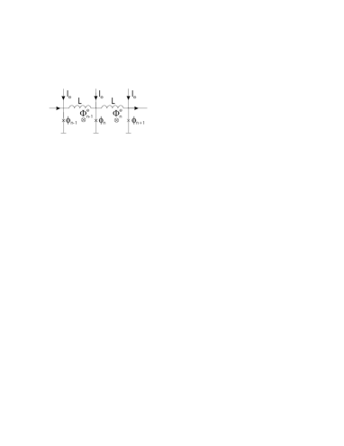
Figure 3: Two elementary cells of the discrete JTL.

In the limit $\alpha=j_{e}=f^{qb}=0$ the exact soliton solution of Eq. (7) has the form

$$\phi_{0}(x,t)=4\tan^{-1}\left[\exp\left(\frac{x-ut-x_{0}}{(1-u^{2})^{1/2}}\right)\right],$$ (10)

where the positive (negative) sign corresponds to a fluxon (antifluxon), $x_{0}$ is the initial position of the soliton, and $u$ its velocity, which can take any value between $-1$ and $1$. To analyze the fluxons dynamics in the JTL following from Eq. (7) in the general case we make use of the collective coordinate perturbation theory developed by McLaughlin and Scott McLaughlin . It is based on the assumption that $j_{e}$, $\alpha\dot{\phi}$, $f^{qb}(\phi,x)\ll 1$, which allows writing the fluxon solution in the form

$$\phi_{0}(x,t;u,X)=4\tan^{-1}\left[\exp\left(\frac{x-X(t)}{(1-u^{2}(t))^{1/2}}\right)\right].$$ (11)

For simplicity we consider here the case where only one fluxon is present in the system.

Without coupling to the qubit, $f^{qb}=0$, the stationary velocity of a fluxon can be derived from the power balance equation McLaughlin , and is given by

$$u_{0}=\left(1+\left(\frac{4\alpha}{\pi j_{e}}\right)^{2}\right)^{-1/2}.$$ (12)

When the qubit is coupled to the JTL, for arbitrary form of the perturbation $f^{qb}(\phi,x)$, the variation parameters $X(t)$ and $u(t)$ obey the differential equations McLaughlin

$$\frac{du}{dt} = \frac{1}{4}\pi j_{e}(1-u^{2})^{3/2}-\alpha u(1-u^{2})-\frac{1}{4}(1-u^{2})$$ (13)

$$\times\int_{-\infty}^{\infty}f^{qb}\left(\phi_{0}(\Theta)\right){\rm sech}\Theta\;dx,$$

$$\frac{dX}{dt} = u-\frac{1}{4}u(1-u^{2})^{1/2}$$ (14)

$$\times\int_{-\infty}^{\infty}f^{qb}\left(\phi_{0}(\Theta)\right)\Theta\;{\rm sech}\Theta\;dx,$$

where $\Theta=(x-X(t))/(1-u^{2})^{1/2}$. In the following section Eqs. (13) and (14) will be solved for both forms of the qubit perturbation $f^{qb}$ given in Eqs. (8) or (9).

Table 1: Parameters of the JTL and the persistent current qubit.

Parameters of JTL Averin ; Savin					$\mid$	Qubit-JTL coupling, k		$\mid$	Parameters of persistent current qubit qubit
$I_{c}$($\mu$A)	$J_{c}$(A/cm2)	$\lambda_{J}$($a$)	$L$(pH)	$\omega_{p}/2\pi$(GHz)	$\mid$	$g\gg\Delta$	$g\ll\Delta$	$\mid$	$\Delta/2\pi$(GHz)	$\epsilon_{max}/2\pi$(GHz)	$L_{qb}$(pH)	$I_{p}$(nA)
0.6	30	2	137	24	$\mid$	0.96	0.05	$\mid$	5.5	55	5	300
2	30	2	41	24	$\mid$	0.53	0.025	$\mid$

III Delay times.

III.1 Qubit far from the Symmetry Point

We first consider the situation where the qubit is prepared far from the symmetry point, $\epsilon_{0}\gg\Delta$. In this case the eigenstates of the qubit are the persistent current states, $|0\rangle$ and $|1\rangle$. For each of them a magnetic flux $\pm MI_{p}$ penetrates the cell of the JTL which is inductively coupled to the qubit. If the size of the qubit is much less than the Josephson penetration depth $\lambda_{J}$ the external magnetic flux in the JTL can be written as

$$\Phi^{e}(x)=\pm MI_{p}\theta(x),$$ (15)

where $\theta(x)$ is the step function, and we assumed the qubit to be located at $x=0$. The corresponding perturbation term in the equation of motion (7) can be written as

$$f^{qb}_{\rm flux}(\phi,x)=\pm\phi^{q}_{1}\delta^{\prime}(x),$$ (16)

where $\phi^{q}_{1}=2\pi MI_{p}/\Phi_{0}$ is the dimensionless qubit-JTL coupling. A thorough experimental and theoretical study of the fluxon dynamics described by the sine-Gordon equation with delta-function terms was performed in Refs. Ustinov ; Malomed for long annular Josephson junctions. Propagation of the charge soliton in 1D array of serially coupled Josephson junction was studied in Ref. charge soliton .

The dimensionless coupling $\phi^{q}_{1}$ depends linearly on the mutual inductance $M$, which for typical experimental conditions is much lower than $1$. Increasing the coupling coefficient $k$ between the qubit loop and the JTL cell enhances the influence of the qubit on the fluxon dynamics in the JTL, but at the same time increases the back-action of the fluxon on the qubit. In particular, the fluxon induces a magnetic flux in the qubit loop, which shifts the working point of the qubit. The persistent current qubit is only well defined when the external flux in the qubit loop is close to the symmetry point $\Phi_{0}/2$. For larger values of the external magnetic flux the form of qubit-JTL perturbation (16) is not valid and a more elaborated model should be used. Moreover, large deviations of the working point can lead to non-adiabatic transitions to higher levels, which also makes the two-level model invalid. In the following we require $MI_{p}I_{L}|_{max}<\epsilon_{max}/2$, where $\epsilon_{max}$ is the maximum value of the energy bias between two persistent current states for which our system is still regarded as the persistent current qubit. This condition translates to the following limitation for the dimensionless coupling

$$\phi_{1}^{q}<\frac{\epsilon_{max}}{\Phi_{0}^{2}a/(\pi^{2}L\lambda_{J})},$$ (17)

and for the coupling coefficient $k=M/\sqrt{LL_{qb}}$,

$$k<\frac{\pi}{2}\left(\frac{\epsilon_{max}\lambda_{J}}{I_{p}\Phi_{0}a}\right)\left(\frac{L}{L_{qb}}\right)^{1/2}.$$ (18)

The right hand side of Eq. (17) is the ratio between the qubit energy splitting and the magnetic energy of a fluxon $\Phi_{0}^{2}a/(\pi^{2}L\lambda_{J})$. It demonstrates that the efficiency of the measurement is low if the magnetic energy of a soliton is much higher than the qubit energy, because one needs to decrease the coupling coefficient $k$ according to (18).

The magnetic energy of a soliton in the JTL can be reduced by decreasing the critical current $I_{c}$ of the junctions. We evaluate the delay times for two specific values of the critical current, $I_{c}=0.6~{}\mu$A and $I_{c}=2~{}\mu$A. Given these values the cell inductance $L$ has to be chosen appropriate to yield suitable values of the Josephson penetration depth $\lambda_{J}$. This length should be large to minimize effects of the discreteness of the JTL, $\lambda_{J}\geq 2a$. On the other hand, it is useful to have $\lambda_{J}$ as small as possible to decrease the magnetic energy of a fluxon and to keep the number of Josephson junctions in the JTL within practical limits. Based on these considerations Averin we choose $\lambda_{J}=2a$. The parameters of the JTL and the qubit which were used in the calculations are listed in Table 1.

From (13-16) we obtain

$$\frac{du}{dt} = \frac{1}{4}\pi j_{e}(1-u^{2})^{3/2}-\alpha u(1-u^{2})$$ (19)

$$\pm\frac{1}{4}(1-u^{2})^{1/2}\phi^{q}_{1}{\rm sech}^{2}\Theta_{0}{\rm sh}\Theta_{0},$$

$$\frac{dX}{dt} = u\pm\frac{1}{4}u\phi^{q}_{1}\left({\rm cosh}\Theta_{0}-\Theta_{0}{\rm sh}\Theta_{0}\right){\rm sech}^{2}\Theta_{0}.$$ (20)

where $\Theta_{0}=X/(1-u^{2})^{1/2}$.

In the ballistic regime, $j_{e}=0$ and $\alpha=0$, we can integrate (19, 20) analytically and obtain the fluxon velocity $u$ and center coordinate $X$ as functions of the parameter $\Theta_{0}$ for the qubit prepared in the eigenstates $|0\rangle$:

$$u(\Theta_{0}) = \left[1-(1-u_{0}^{2})\left(\frac{\phi^{q}_{1}+4{\rm cosh}\Theta_{0}}{4{\rm cosh}\Theta_{0}}\right)^{2}\right]^{1/2},$$ (21)

$$X(\Theta_{0}) = \Theta_{0}(1-u_{0}^{2})^{1/2}\left(1+\frac{\phi^{q}_{1}}{4{\rm cosh}\Theta_{0}}\right).$$ (22)

The solution for the state $|1\rangle$ is obtained by replacing $\phi^{q}_{1}$ by $-\phi^{q}_{1}$.

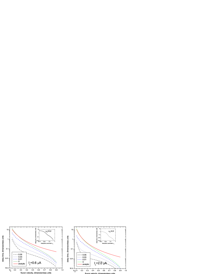
Figure 4: Delay time of a soliton induced by the qubit as a function of initial soliton velocity $u_{0}$ when the qubit is far from the symmetry point, $\epsilon_{0}\gg\Delta$. The velocity and time are measured in units of $\lambda_{J}\omega_{p}$ and $\omega_{p}^{-1}$, respectively. Four curves are obtained numerically from Eqs. (13, 14) for different values of the dissipation strength $\alpha$ (shown in the legend box). The red solid line shows the analytical solution (25). The parameters of the JTL and the persistent current qubit are listed in Table 1. The inset shows the dependence of the delay time on the dissipation strength $\alpha$ for the initial soliton velocity $u_{0}=0.2$.

To proceed we first consider the situation, where the soliton is able to pass the potential and, therefore, we can always introduce the delay time caused by the perturbation due to the qubit as

$$t_{d} = |t_{|0\rangle}-t_{|1\rangle}|=2|t_{|0\rangle}-t_{0}|$$ (23)

$$=\frac{2}{u_{0}}\int_{-\infty}^{\infty}\left|\frac{u_{0}-u(X)}{u(X)}\right|dX.$$

Here $t_{|0\rangle}$ and $t_{|1\rangle}$ are the propagation times corresponding to the two persistent current states of the qubit, and $t_{0}$ is the value without qubit interaction. The factor $2$ in Eq. (23) reflects the fact that the perturbation $f^{qb}_{\rm flux}$ has the same magnitude but different signs for the two persistent current states. When the velocity is only slightly perturbed by the qubit, $\varepsilon_{1}=(1-u_{0}^{2})\phi^{q}_{1}/(4u_{0}^{2})\ll 1$, we find

$$u(\Theta_{0})=u_{0}\left(1-\varepsilon_{1}{\rm sech}\Theta_{0}\right)+o(\varepsilon_{1}^{2}).$$ (24)

The delay time (23) can then be evaluated as

$$t_{d}=\frac{2\varepsilon_{1}}{u_{0}^{2}}\int_{-\infty}^{\infty}\varepsilon_{1}{\rm sech}\left(\frac{X}{(1-u_{0}^{2})^{1/2}}\right)dX\simeq\frac{\pi\phi^{q}_{1}}{2u_{0}^{3}},$$ (25)

where the last part of the equation describes the “non-relativistic case” $u_{0}\ll 1$.

From (21) we see that for $\phi^{q}_{1}/4>(1-u_{0}^{2})^{-1/2}-1$ the soliton does not have enough kinetic energy to pass the potential barrier induced by the the qubit in the state $|0\rangle$. After approaching the qubit the soliton will be reflected by the barrier. Due to the combination of dissipation and driving the soliton will oscillate and eventually stop at the “pinning point” where $u=0$ and $\dot{X}=0$. The pinning of a fluxon and can also be used for the transmission detection mode of measurement, but will not be analyzed here further.

The results of a numerical evaluation of the delay times for the JTL with dissipation are presented in Fig. 4. As expected the analytical formula (25) gives a good estimate even for intermediate values of the soliton velocity $u_{p}\ll u_{0}\ll 1$, where $u_{p}$ is the minimal possible velocity for which a fluxon is still able to pass the potential barrier created by the qubit.

Another observation is, that for fixed value of the soliton velocity $u_{0}$ the delay time decreases with increasing strength of the dissipation $\alpha$. This property is displayed by Fig. 5, which shows the velocity as a function of the soliton coordinate for different values of $\alpha$. One can see that with increasing dissipation the fluxon velocity deviates from the dissipationless solution (13,14). The initial decline of the fluxon velocity becomes less effective and is also partially compensated by the following acceleration of the fluxon. The compensation is the more complete the higher is the dissipation, which leads to zero delay times in the limit of strong dissipation. This behavior is typical for the particle driven in viscous media and can be understood from power balance considerations. Let us consider the case when the qubit induces a positive potential barrier for a fluxon. When a fluxon is moving with stationary velocity far from the qubit its energy gain and losses are equal. Approaching the potential barrier the velocity of a fluxon decreases, which leads to a reduction in energy losses due to dissipation. However, the gain of energy due to driving stays on the same level. As a result a fluxon receives an excess amount of energy, which later leads to an increase of the fluxon velocity above the initial value. Thus, we can use the dissipationless solution as an approximation for evaluating the delay times of a fluxon only if $\alpha<\phi^{q}_{1}$. For $\alpha>\phi^{q}_{1}$ the delay times degrade rapidly with increasing $\alpha$. We expect that the delay times can be reliably detected only if $\alpha\lesssim\phi^{q}_{1}$. This establishes another limitation to the parameters of the JTL for the case of very weak qubit-JTL coupling.

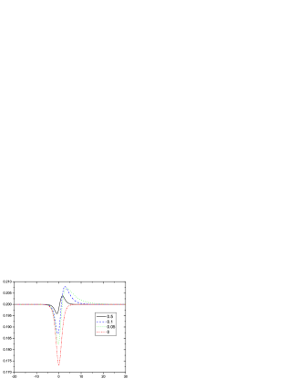
Figure 5: Fluxon velocity as function of its coordinate for different values of the dissipation strength $\alpha$ (shown in the legend box)

.

Next we consider the situation when the qubit is initially prepared at the symmetry point but shifted far from it by the moving fluxon. In what follows we will show that this regime is approximately equivalent to that when the qubit is kept far from the symmetry point all the time, and we can use the previous results for the delay time. Indeed for typical parameters of the JTL and chosen inductive coupling we have $g\gg\Delta$, which proves that even if the qubit is initially prepared at the symmetry point, $\epsilon_{0}=0$, it is shifted far from it by the flux induced in the qubit loop by the moving fluxon. At the symmetry point the persistent current in the qubit loop is zero, and the qubit induces no magnetic flux in the JTL cell, $I_{L}(t)=0$. As soon as the approaching fluxon shifts the qubit from the symmetry point, $2MI_{p}I_{L}(t)\sim\Delta$, the persistent current is no longer zero. The maximum value of the persistent current, $I_{p}$, is reached once the qubit is pushed far away from the symmetry point, $2I_{p}MI_{L}(t)\gg\Delta$. When the fluxon moves away the qubit returns to the symmetry point with zero persistent current in its loop. These considerations, of course, are valid only if the qubit was prepared in an energy eigenstate and if the shift by the fluxon occurs adiabatically. The qubit affects the fluxon dynamics only during the period of time $\sim\lambda_{J}/u_{0}$ when the fluxon is moving close to the qubit. Most of this time the qubit is already shifted far from the symmetry point and induces the perturbation to the fluxon motion according to Eq. (8). The quick switching of the persistent current from zero to $I_{p}$ and back in the initial and final stages of the qubit-JTL magnetic flux exchange yield only a small contribution to the overall delay time experienced by the fluxon. Therefore, we can use the calculated delay times shown in Fig. 4 even if the qubit is initially prepared at the symmetry point for $g\gg\Delta$. However, we need to evaluate the probability of non-adiabatic transitions of the qubit to another eigenstate, which creates an additional source of error for the measurement. These results will be presented in Section IV.

III.2 Qubit at the Symmetry Point

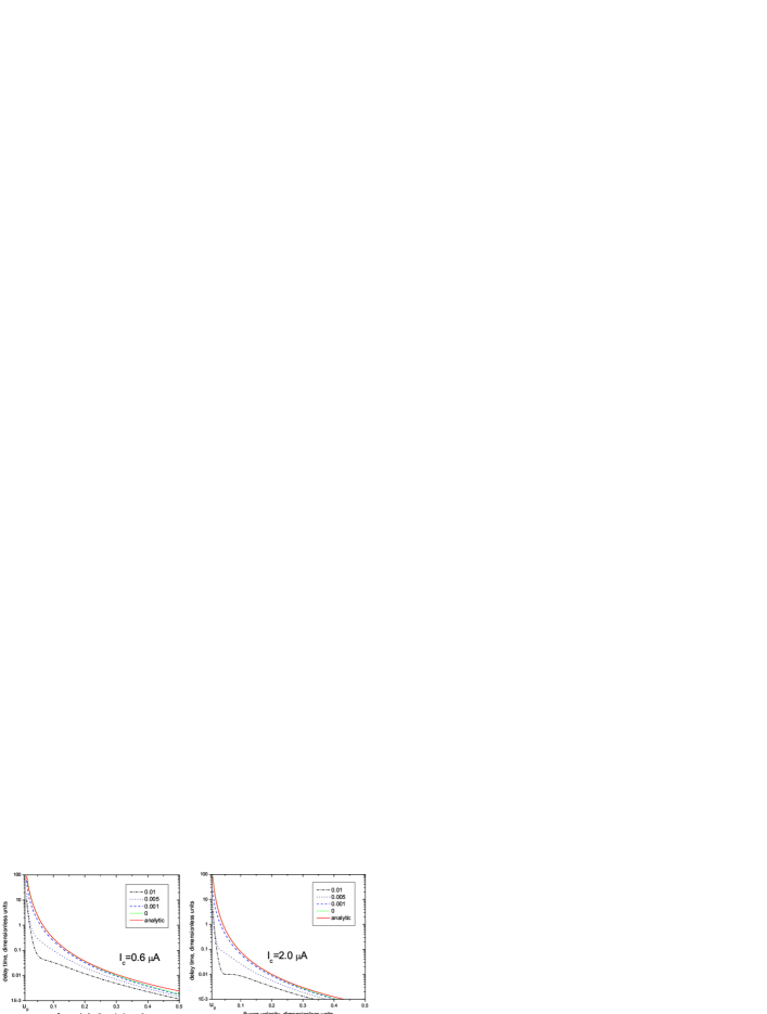
Figure 6: Delay time of a soliton induced by the qubit as function of the initial soliton velocity $u_{0}$ when the qubit remains at the symmetry point $\epsilon_{0}=0$. The velocity and time are measured in units of $\lambda_{J}\omega_{p}$ and $\omega_{p}^{-1}$, respectively. Four curves are numerical solutions of Eqs. (13, 14) for different values of the dissipation strength $\alpha$ (shown in the legend box). The red solid curve shows the analytical solution (34). The parameters of the JTL and persistent current qubit are given in Table 1. The coupling coefficient between the qubit loop and the cell of the JTL is $k=0.05$ which leads to the dimensionless coupling $\phi^{q}_{1}=3\times 10^{-4}$ in the sine-Gordon equation. The value of the coupling coefficient is reduced in order to keep the qubit all the time at the symmetry working point.

In this subsection we consider the situation where the qubit is prepared initially at the symmetry point $\epsilon_{0}=0$ and remains nearby during the measurement. This requires that the coupling between qubit and JTL is weak and $g\ll\Delta$ to ensure that a soliton does not shift the qubit from the symmetry point significantly. As a consequence the expectation value of the flux in the energy eigenstates of the qubit is close to zero. If the coupling term (5) varies slowly we can treat the sum $H_{qb}+H_{I}$ in an adiabatic approximation and diagonalize it to obtain

$$H_{qb}+H_{I} = \rho_{z}\sqrt{\Delta^{2}/4+M^{2}I_{p}^{2}I_{L}^{2}(t)}$$

$$\simeq\frac{\Delta}{2}\rho_{z}+\frac{L_{eff}I_{L}^{2}(t)}{2}\rho_{z}=H_{qb}^{adiab}+H_{I}^{adiab},$$

where $L_{eff}=2I_{p}^{2}M^{2}/\Delta$. The approximation is valid if $P\ll 1$, where $P$ is the probability of Landau-Zener transition between energy eigenstates due to time dependence of $I_{L}(t)$, which is calculated in the next section.

The interaction term $H_{I}^{adiab}$ indicates that the qubit-JTL interaction in the adiabatic approximation is equivalent to the change of the inductance of the JTL cell which is coupled to the qubit by the additional value of $L_{eff}$ whose sign depends on the energy eigenstate of the qubit. This property can be used for the read out of the qubit when it is always kept at the symmetry point $\Phi=\Phi_{0}/2$.

The qubit-JTL interaction $H_{I}^{adiab}$ leads to the following perturbation term in the sine-Gordon equation (7)

$$f^{qb}_{\rm ind}(\phi,x)=\pm\phi^{q}_{2}\frac{\partial}{\partial x}\left[\delta(x)\phi_{x}\right],$$ (27)

where $\phi^{q}_{2}=L^{eff}a/(L\lambda_{J})$ is the corresponding dimensionless qubit-JTL coupling and $\pm$ correspond to the eigenstates $|\pm\rangle=(1/\sqrt{2})(|0\rangle\pm|1\rangle)$.

The Hamiltonian (III.2) is valid only for $g\ll\Delta$, which establishes the condition for the maximum possible dimensionless coupling

$$\phi_{2}^{q}\ll\frac{\Delta/2}{\Phi_{0}^{2}a/(\pi^{2}L\lambda_{j})},$$ (28)

and coupling coefficient

$$k\ll\frac{\pi}{2}\left(\frac{\Delta\lambda_{J}}{I_{p}\Phi_{0}a}\right)\left(\frac{L}{L_{qb}}\right)^{1/2}.$$ (29)

In order to keep the qubit at the symmetry point for the chosen parameters of the qubit and the JTL (shown in Table 1) the coupling coefficient should satisfy: $k\ll 0.096$ for $I_{c}=0.6~{}\mu$A and $k\ll 0.053$ for $I_{c}=2.0~{}\mu$A. For the calculation we take $k=0.05$ and $k=0.025$ which leads to $\phi^{q}_{2}=3\times 10^{-4}$ and $\phi^{q}_{2}=8\times 10^{-5}$, respectively.

From (13,14) and (27) we obtain

$$\frac{du}{dt} = \frac{1}{4}\pi j_{e}(1-u^{2})^{3/2}-\alpha u(1-u^{2})$$ (30)

$$\pm\frac{\phi^{q}_{2}}{2}{\rm sech}^{2}\Theta_{0}{\rm tanh}\Theta_{0},$$

$$\frac{dX}{dt} = u\pm\frac{\phi^{q}_{2}}{2}\frac{u\;{\rm sech}^{2}\Theta_{0}}{(1-u^{2})^{1/2}}\left(1-\Theta_{0}{\rm tanh}\Theta_{0}\right).$$ (31)

For $\alpha=j_{e}=0$ in the non-relativistic limit $u\ll 1$ one can evaluate for the qubit in the eigenstate $|+\rangle$

$$u^{2}=u_{0}^{2}-\frac{\phi^{q}_{2}}{2}{\rm sech}^{2}X,$$ (32)

and

$$u\simeq u_{0}\left(1-\varepsilon_{2}{\rm sech}^{2}X\right)+o(\varepsilon_{2}^{2}),$$ (33)

where $\varepsilon_{2}=\phi^{q}_{2}/(4u_{0}^{2})$. The pinning of the fluxon occurs if $u_{0}^{2}<\phi^{q}_{2}/2$. We can calculate the delay time according to (23) as

$$t_{d}=\frac{2\varepsilon_{2}}{u_{0}}\int_{-\infty}^{\infty}{\rm sech}^{2}XdX=\frac{\phi^{q}_{2}}{u_{0}^{3}}.$$ (34)

The results of the numerical evaluation of the delay times in this regime are shown in Fig. 6. For the same values of the fluxon speed the delay times are smaller as compared to Fig. 4. However, since the pinning of a soliton occurs at slower velocities we can, in principle, achieve larger values of the delay times.

IV Back-action of a Fluxon on the Qubit

The back-action of a fluxon on the qubit produces several effects including dephasing of the qubit in the measurement basis Averin2 and a shift of the working point of the qubit. Dephasing, i.e., the decay of the off-diagonal elements of the density matrix of the qubit in the measurement basis, does not affect the measurement outcomes studied here dephasing and is not considered further.

In contrast, the shift of the working point of the qubit can potentially “destroy” the qubit and, furthermore, induce non-adiabatic transitions between the qubit states. Both processes create errors in the measurement and should be taken into account. By restricting the qubit-JTL coupling according to (18) or (29) we insure that the system remains a persistent current qubit during the whole time of the measurement. In this section we derive the probability of non-adiabatic transition between eigenstates of the qubit due to a passing fluxon. It should be noted that non-adiabatic transitions are a potential problem only if the qubit is initially prepared at the symmetry point. Far from the symmetry point the Hamiltonian of the qubit (2) and the interaction Hamiltonian (5) approximately commute and non-adiabatic transitions are negligible.

In order to study nonadiabatic transitions we assume that the qubit is initially prepared in the excited state $|-\rangle$ at the symmetry point $\epsilon_{0}=0$ where its unperturbed dynamics is described by the Hamiltonian $H_{qb}=-(\Delta/2)\sigma_{x}$. For a fluxon passing the qubit the time-dependent qubit-JTL coupling can be written according to (5) and (10) as

$$H_{I} = MI_{p}I_{L}(t)\sigma_{z}$$

$$= -\frac{MI_{p}\Phi_{0}}{\pi L(\lambda_{J}/a)\sqrt{1-u^{2}_{0}}}\;{\rm sech}\left(\frac{u_{0}t}{\sqrt{1-u_{0}^{2}}}\right)\sigma_{z}.$$

Here we neglected the action of the qubit on the fluxon. The transition probability from the excited state $|-\rangle$ to the ground state $|+\rangle$ induced by one passing fluxon is then given by Zener

$$P=MI_{p}(2\hbar)^{-2}\left|\frac{\sin A}{A}\int^{\infty}_{-\infty}I_{L}(t)e^{it\Delta/\hbar}dt\right|^{2},$$ (36)

where $A=MI_{p}(2\hbar)^{-2}\int^{\infty}_{-\infty}I_{L}(t)dt$. After inserting (IV) we obtain

$$P=\sin^{2}\left(\frac{I_{p}M\Phi_{0}}{L(\lambda_{J}/a)u_{0}\hbar\omega_{p}}\right){\rm sech}^{2}\left(\frac{\pi\sqrt{1-u_{0}^{2}}\Delta}{2u_{0}\omega_{p}}\right).$$ (37)

We will use this result to evaluate the measurement efficiency in Section VII.

V Soliton Jitter

In order to be detected the delay time should exceed the time fluctuations induced by thermal noise in the JTL. We can account for thermal noise by adding a stochastic term $\xi(x,t)$ to the sine-Gordon equation (7),

$$\ddot{\phi}-\phi_{xx}+\sin\phi=j_{e}-\alpha\phi_{t}-\xi(x,t).$$ (38)

The noise is assumed to be white with autocorrelation function

$$\langle\xi(x,t)\xi(x^{\prime},t^{\prime})\rangle=16\alpha(k_{B}T/E_{0})\delta(x-x^{\prime})\delta(t-t^{\prime}).$$ (39)

Here $E_{0}=8\left(\hbar J_{c}\lambda_{J}/2e\right)$ is the rest energy of a soliton, and the coefficient $16\alpha(k_{B}T/E_{0})$ is fixed by the fluctuation-dissipation theorem Salerno . The noise spectral density for the fluxon velocity is given by joergensen ; Salerno

$$S_{\Delta u}(\omega)=\frac{2\alpha k_{B}T}{E_{0}}\frac{(1-u_{0}^{2})^{5/2}}{\alpha^{2}+\omega^{2}},$$ (40)

where $\Delta u(t)=u(t)-u_{0}$. Starting from the initial condition that at $t=0$ the velocity of the fluxon is controlled and equal to $u_{0}$ we find the velocity autocorrelation function to be given by

$$\langle\Delta u(t_{1})\Delta u(t_{2})\rangle = \frac{k_{B}T}{E_{0}}(1-u_{0}^{2})^{5/2}$$ (41)

$$\times\left(e^{-\alpha|t_{1}-t_{2}|}-e^{-\alpha|t_{1}+t_{2}|}\right).$$

The uncertainty in the velocity of the fluxon leads to an uncertainty of its coordinate $\Delta X(t)=\int_{0}^{t}\Delta u(t^{\prime})dt^{\prime}$ and propagation time $\Delta t=\Delta X/u_{0}$. The time jitter of the fluxon, defined as the standard deviation of the propagation time $\delta t\equiv\left(\langle\Delta t^{2}\rangle\right)^{1/2}$, is then given by

$$\delta t = \left(\frac{2k_{B}T}{\alpha^{2}E_{0}}\right)^{1/2}\frac{(1-u_{0}^{2})^{5/4}}{u_{0}}$$ (42)

$$\times\left(t\alpha+e^{-\alpha t}-1-\frac{1}{2}\left(1-e^{-\alpha t}\right)^{2}\right)^{1/2}.$$

Limiting cases of Eq. (42) are $\delta t\propto t^{1/2}$ in the diffusive regime $\alpha t\gg 1$, and $\delta t\propto t^{3/2}$ in the ballistic regime $\alpha t\ll 1$. The time jitter (42) leads to further errors in the measurement procedure, which will be analyzed in section VII.

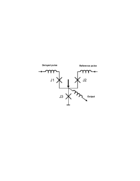
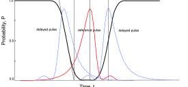
(a) (b)

Figure 7: (a) Schematic of RSFQ confluence buffer, and (b) the probability of double switching of output junction J3.

VI RSFQ delay detector

Before turning to a quantitative analysis of the measurement errors we describe in this section an RSFQ delay detector that is need to measures the time between two SFQ pulses propagating through a JTL. We first evaluate the time resolution of a single RSFQ decision gate and the time resolution of the improved detector based on a time vernier. Based on realistic parameters we estimate the hardware complexity of the detector and discuss possible designs of the circuit presently developed experimentally VTT .

The operation of any RSFQ gate is based on the time resolution between SFQ pulses. The gates produce binary output depending on the relative time between either clock and data pulses or between two input data pulses. The simplest RSFQ gate that can be used as a decision circuit is the asynchronous OR or confluence buffer shown in Fig. 7. The figure also illustrates the operation of the confluence buffer as a time detector. A single SFQ pulse on either input produces a SFQ pulse on output. Therefore, for delayed input pulses two output SFQ pulses are produced. In case of simultaneous arrival the input pulses compensate each other resulting in a single SFQ pulse on output. Such behavior of the RSFQ confluence buffer is well known and has been experimentally verified many times, see for example Ref. Bunyk97 .

In general, the time resolution of any RSFQ gate is determined by the resolution of the balanced comparator formed by two junctions connected in series. In the confluence buffer balanced comparators are formed by junctions J1, J3 or J2, J3. The probability of junction switching in the comparator obeys a normal distribution with $\sigma_{c}\approx 0.13t_{SFQ}$, where $t_{SFQ}$ is the width of SFQ pulse Ortlep06 ; Filippov99 . In time units normalized to $1/\omega_{p}$, the width of the SFQ pulse is approximately

$$t_{SFQ}\approx 6\frac{1}{\sqrt{\beta_{c}}},$$ (43)

where $\sqrt{\beta_{c}}=\omega_{c}/\omega_{p}$ is the McCumber-Stewart parameter. The corresponding normalized one-sigma jitter of a single decision gate with $\beta_{c}=2$ is

$$\sigma_{c}=0.13t_{SFQ}\approx 0.78\frac{1}{\sqrt{\beta_{c}}}\approx 0.55.$$ (44)

For a measurement error of $10^{-2}$ the time resolution of a single RSFQ gate, $t_{r}^{g}$, is given by $4\sigma_{c}$ and equal to $t_{r}^{g}=2.2$. This time resolution does not dependent on the temperature since the measurement involves symmetric stochastic processes of the switching of two balanced junctions HerrIsec .

As it is shown in Section III, the delay time between SFQ pulses that needs to be detected is in the range of $t_{d}=0.1-5$ depending on the actual dissipation in long JTLs and the accuracy in fixing the initial fluxon velocity. In order to improve the time resolution of the RSFQ delay detector time a vernier with $N$ decision gates can be used Kirichenko01 ; Fujimaki06 , the block diagram of which is shown in Fig. 8. After the JTLs, both pulses propagate through the chain of splitters and arrive on a chain of $N$ decision gates with inputs delayed in time by $t_{d}$. The operation principle of the time vernier is the same as that of a multibit analog-to-digital converter where each bit compares the signal with a slightly shifted threshold. In accordance with the standard theory for analog-to-digital converters the resolution improves as the square root of the number of bits ADC .

Time resolution of the vernier is $t_{r}^{v}=t_{r}^{g}/\sqrt{N}$ and relative time difference between stages of the vernier is $t_{s}=t_{r}^{g}/N$. The error of time measurements depends on the ratio between time difference, $t_{s}$, and jitter accumulated in the pulse pathes, $\sigma_{v}$,

$$P_{err}=\frac{1}{2}{\rm erfc}(\frac{t_{s}}{\sigma_{v}}).$$ (45)

The accumulated jitter is

$$\sigma_{v}=\sqrt{2*N_{v}}\sigma_{J},$$ (46)

where $N_{v}$ is number of Josephson junctions in each pulse path and $\sigma_{J}$ is a jitter per Josephson junction. The factor two comes from the fact that there are two chains of splitters involved. The number of Josephson junctions in the splitter chain grows like $N_{v}=N\log N$. The single junction jitter at 4.2 K is about $\sigma_{J}=0.015t_{SFQ}$ Ortlep06 and it scales as square root of temperature and as square root of shunts resistors of the junction.

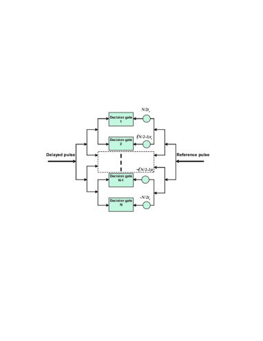
Figure 8: Block diagram of a RSFQ time vernier.

Typical operating bath temperatures for the qubit experiments are about 30 mK. For process with operating frequency below 5  GHz and assuming use of cooling fins for thermalization of the hot electrons in the normal metal shunts, the effective noise temperature of the RSFQ gates can be reduced down to 80 mK for a 30 A/cm² process and to 30 mK for a 10 A/cm² process Ohki06 . The temperature range between 30-80 mK corresponds to one-sigma jitter of $\sigma_{J}=0.0012-0.0004$ for a single Josephson junction with $\beta_{c}=2$.

For measurement errors of $10^{-2}$ the time resolution of the RSFQ time vernier is given by $4\sigma_{v}$ that results in the following relation for the optimum number of stages,

$$\frac{4\sigma_{c}}{N}=4\sqrt{2*N\log N}\sigma_{J}.$$ (47)

Equation (47) gives $N=40$ and corresponding $t_{r}^{v}=0.33$ for 30 mK (10 A/cm² process) and $N=20$ and corresponding $t_{r}^{v}=0.5$ for 80 mK (30 A/cm² process).

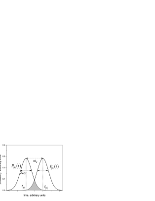
Figure 9: Sketch of the distribution functions which describe the propagation time of a soliton. The two functions $P_{|0\rangle}(t)$ and $P_{|1\rangle}(t)$ are peaked around the average values of the propagation times $t_{|0\rangle,|1\rangle}$ corresponding to the different eigenstates of the qubit $|0\rangle$ and $|1\rangle$. The standard deviation and peak separation are given by $\sqrt{n}\,\delta t$ and $n\,t_{d}$, respectively. The overlap of the distribution functions (grey color) indicates the regime where the measurement yields an error.

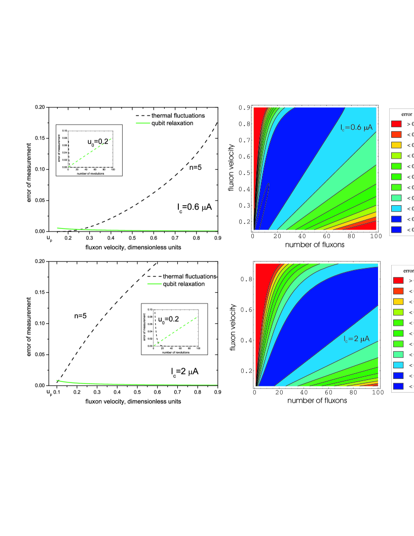
Figure 10: Different contributions to the measurement error for $L_{r}=25\lambda_{J}$, $T=20\;{\rm mK}$, $\alpha=0.001$. The upper plots correspond to $I_{c}=0.6~{}\mu$A and $k=0.96$ while for the lower plots $I_{c}=2~{}\mu$A and $k=0.53$. The qubit is initially prepared far from the symmetry point. See text for detailed explanations.

VII Measurement errors

In an experimental implementation the length $L_{JTL}$ of the JTL is finite. For $L_{JTL}\gg\lambda_{J}$ the delay time of a fluxon induced by the qubit is that of the infinite JTL shown in Figs. 4 and 6. The time jitter of a fluxon at the end of the JTL is given by Eq. (42) with $t=L_{JTL}/u_{0}$. Due to the jitter the propagation time of a soliton will be scattered around the average values $t_{|0\rangle}$ and $t_{|1\rangle}$ corresponding to the different energy eigenstates of the qubit $|0\rangle$ and $|1\rangle$ if the qubit is far from the symmetry point. (A similar analysis holds for distinguishing the states $|+\rangle$ and $|-\rangle$ if the qubit is at the symmetry point.) We can introduce the corresponding distribution functions $P_{|0\rangle}(t)$ and $P_{|1\rangle}(t)$ for the propagation time of a soliton, which have maxima at $t_{|0\rangle}$ and $t_{|1\rangle}$, separated by the delay time $t_{d}$ and whose standard deviations are equal to the jitter $\delta t$. The overlap of the two distribution functions $P_{|0\rangle}(t)$ and $P_{|1\rangle}(t)$ characterizes the potential to distinguish the two eigenstates of the qubit. For a normal distribution the area of the overlap and the associated error of the measurement are erfc$[t_{d}/\left(2\sqrt{2}\delta t\right)]$ and (1/2)erfc$[t_{d}/\left(2\sqrt{2}\delta t\right)]$, respectively. For experimentally relevant case of large separation of the distribution functions, $t_{d}\gg\delta t$, the error can be approximated by $\left(\sqrt{2}\delta t/t_{d}\right)\exp\left(-t_{d}^{2}/8\delta t^{2}\right)$. The ratio of the delay time to the jitter, which determines the error of measurement due to thermal fluctuations, can be estimated for a JTL with low dissipation, $\alpha\ll\phi^{q}_{1,2}$, according to the expressions (25), (34) and (42) as

$$\frac{t_{d}}{\delta t}\propto\frac{\pi\phi^{q}}{2u_{0}^{3/2}}\left(\frac{E_{0}\alpha}{2k_{B}TL_{JTL}}\right)^{1/2}.$$ (48)

This results suggests that in order to decrease the effect of thermal noise it is favorable to use slower fluxons. On the other hand, low velocity fluxons can be difficult to produce and control technologically. To avoid pinning by the qubit we also cannot choose the speed of the fluxons too small.

For realistic experimental situations some of the magnetic flux from the control circuit of the qubit $\Phi_{ext}$ penetrates the JTL and create an additional potential barrier for fluxons. If the external flux $\Phi_{ext}$ is much smaller than the flux quantum $\Phi_{0}$ we can again use the collective perturbation theory to analyze its effect on the delay time. According to the definition (23) there is no effect of $\Phi_{ext}$ on the difference in the delay times since the potential barrier does not depend on the qubit quantum state. However, for $\Phi_{ext}>MI_{p}$ the pinning velocity of a fluxon will be larger. This should be taken into account and can affect the measurement because low fluxon velocities could be no longer accessible.

For further improvement of the signal-to-noise ratio one can use $n$ fluxons, sending them to the JTL one after another. After $n$ fluxon passings the sum of the delay times and separation of the peaks of the distribution functions will scale linearly as $n\,t_{d}$, but the jitter will increase only as $\sqrt{n}\,\delta t$, and the resulting measurement error decreases according to $(1/2){\rm erfc}[\sqrt{n}t_{d}/\left(2\sqrt{2}\delta t\right)]$.

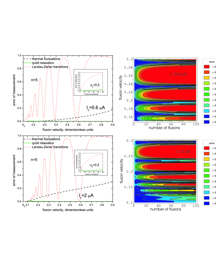
Figure 11: Different contributions to the measurement error for $L_{JTL}=25\lambda_{J}$, $T=20\;{\rm mK}$, $\alpha=0.001$. The upper plots correspond to $I_{c}=0.6~{}\mu$A and $k=0.96$ while for the lower plots $I_{c}=2~{}\mu$A and $k=0.53$. The qubit is initially prepared at the symmetry point but is shifted far from it by a moving soliton. See text for detailed explanations.

The qubit also experiences other sources of noise during the measurement which are not related to the JTL. Their effect can be described phenomenologically by two characteristic time scales: the relaxation time $T_{1}$ and the decoherence time $T_{2}$. The pure decoherence, i.e., the decay of the off-diagonal elements of the density matrix of the qubit, has no effect on the measurement outcome and is not relevant in our case. The relaxation changes the probability distribution described by the diagonal elements of the density matrix and, thus, affects the measurement. For a qubit initially prepared in the excited state, after $n$ passings fluxons the probability to find the qubit in the ground state is $1-\exp(-nL/(u_{0}T_{1}))$. We take this probability as the approximate (upper bound) measure of the possible error of measurement due to relaxation of the qubit.

Table 2: Error of measurement by a single fluxon for $L_{JTL}=25\lambda_{J}$, $T=20\;{\rm mK}$, $u_{0}=0.2$, $\alpha=0.001$.

	Variant 1	Variant 2	Variant 3
$I_{c}$($\mu$A)	0.6	2	0.6
k	0.93	0.53	0.05
$t_{d}$($\omega_{p}^{-1}$)	4.5	1.2	0.04
$\delta t$($\omega_{p}^{-1}$)	1.5	0.84	1.5
Errors of measurement (in $\%$)
jitter	7	24	50
relaxation	0.08	0.08	0.08
LZ transitions, $\epsilon_{0}=0$	2	2	6.8
total error, $\epsilon_{0}\gg\Delta$	7	24	-
total error, $\epsilon_{0}=0$	9	26	55

Finally, if measure the qubit at the symmetry point there is an additional error associated with Landau-Zener transitions between the qubit eigenstates. Following considerations similar to the previous paragraph we define the measure of the error due to Landau-Zener transitions as $1-\exp(-nP)$ where probability $P$ is given by (37).

The efficiency of the qubit measurement by a single fluxon is given in Table 2. The qubit can be measured at the symmetry point and far from it with accuracy of approximately $90\%$ for $I_{c}=0.6~{}\mu$A and $75\%$ for $I_{c}=2~{}\mu$A. To improve the accuracy one needs to use many fluxons. Figs. 10 and 11 show the error of the measurement for the qubit initially prepared far from symmetry point and at the symmetry point, respectively. The total errors of the measurements are shown on the right contour plots as a function of the number of fluxons passings and the initial velocity of the fluxons. They are estimated as $1-\exp\left[-{\rm erfc}(\sqrt{n}t_{d}/2\sqrt{2}\delta t)-nL/(u_{0}T_{1})\right]$ for Fig. 10 and $1-\exp\left[-{\rm erfc}(\sqrt{n}t_{d}/2\sqrt{2}\delta t)-nL/(u_{0}T_{1})-nP\right]$ for Fig. 11. The different contributions to the total error are also plotted separately as a function of the fluxon velocity (the left plots) and number of fluxon passings (the insets of the left plots). The non-adiabatic transitions are suppressed if the qubit is prepared far from the symmetry point, hence there is no curve related to Landau-Zener transitions in Fig. 10. One can see that for high fluxon velocities the measurement quality is limited by the jitter and the Landau-Zener transition probability (if the qubit is at the symmetry point). For low velocities the measurement time increases and the relaxation of the qubit becomes also important. Under optimum conditions the qubit can be measured with probability of error below $1\%$ far from symmetry point and below $7\%$ at the symmetry point with the measurement time of approximately $4$ ns.

Fig. 12 shows the measurement error for $L_{JTL}=25\lambda_{J}$, $T=20\;{\rm mK}$, $\alpha=0.001$ and $k=0.05$. The qubit stays at the symmetry point during complete measurement. The coupling coefficient is chosen small to prevent a shift of the qubit from the symmetry point by the passing soliton. Thus, the influence of the qubit on a soliton is also weak, which affects the sensitivity of the measurement. From Fig. 12 it becomes clear that in order to achieve better measurements we need low soliton speed and a large number of fluxons passings. As a result the time of measurement which is required to extract the information about the qubit quantum state is comparable to the relaxation time of the qubit. This makes it impossible to efficiently measure a qubit in this regime for the chosen parameters of the JTL. A reduction of the critical current of the Josephson junctions may allow decreasing the magnetic energy of the solitons and consequently increase the coupling coefficient. In this case the accuracy of the measurement will be improved while the qubit will remain all the time at the symmetry point.

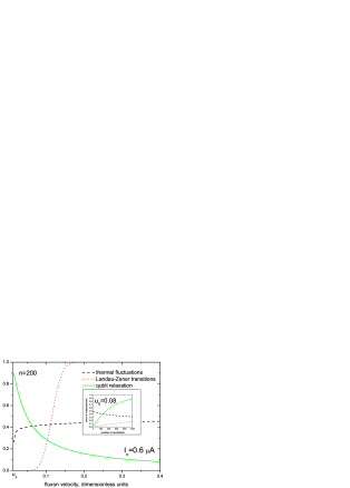
Figure 12: Different contributions to the error of a measurement for $L_{JTL}=25\lambda_{J}$, $T=20\;{\rm mK}$, $\alpha=0.001$, $I_{c}=0.6~{}\mu$A and $k=0.05$. The qubit stays at the symmetry point during the measurement.

VIII Summary

In summary, we analyzed the measurement process of a quantum state of a flux qubit by solitons propagating in an underdamped JTL. The coupling between the qubit and the JTL is inductive. We focused on the regime in which the information about the measured state is stored in the delay time of JTL solitons passing by (scattering from) the qubit. If the qubit is in an energy eigenstate far from the symmetry point its persistent current induces an external magnetic flux in the JTL which serves as a scattering potential for the JTL solitons. Two eigenstates induce different (opposite) scattering potentials, thus producing different delay times. A similar measurement mechanism works when the qubit is prepared at the symmetry point but, due to strong coupling, each passing soliton pushes the qubit far from the symmetry point.

We have demonstrated that the delay times are longer for lower magnetic energies and velocities of the fluxons and lesser dissipation in the JTL. Since the Josephson penetration depth is fixed by the design requirement $\lambda\approx 2a$ the only possibility to reduce the magnetic energy of the soliton is to decrease the Josephson junction critical currents $I_{c}$. For low critical currents $I_{c}=0.6~{}\mu$A and $I_{c}=2.0~{}\mu$A the delay times are in the range $t_{d}=0.1-10\omega_{p}^{-1}$ which can be reliably detected by the RSFQ delay detector. The major sources of the measurement errors are the propagation time uncertainty of a fluxon due to thermal noise in the JTL and the intrinsic qubit relaxation. Non-adiabatic transitions between the energy eigenstate induced by fluxons can cause an additional error if the qubit is measured at the symmetry point. For a JTL consisting of 50 elementary cells, dissipation strength $\alpha=0.001$, temperature $T=20$ mK, fluxon velocity $u_{0}=0.2$, and coupling coefficient $k\sim 1$ the measurement errors of the qubit by a single fluxon are $9\%$ and $26\%$ for $I_{c}=0.6~{}\mu$A and $I_{c}=2.0~{}\mu$A, respectively. In order to increase the signal-to-noise ratio one can use many fluxons which results in the improved accuracy of measurement exceeding $99\%$ for the qubit far from the symmetry point and $90\%$ at the symmetry point.

For weak qubit-JTL coupling, $k\ll 0.01$, a qubit prepared at the symmetry point stays there all the time and induces no magnetic field in the JTL. In this case the measurement can be based on the fluxon scattered by the potential associated with the change of the effective inductance of that JTL cell which is coupled to the qubit loop. We found that a further reduction of the critical current of the Josephson junction is required for an effective measurement in this regime.

- (1) D. V. Averin, K. Rabenstein, and V. K. Semenov, Phys. Rev. B 73, 094504 (2006).
- (2) V. K. Kaplunenko and A. V. Ustinov, Eur. Phys. J. B 38, 3 (2004).
- (3) J. E. Mooij, T. P. Orlando, L. Levitov, L. Tian, C. H. van der Wal, and S. Lloyd, Science 285, 1036 (1999).
- (4) T. P. Orlando, J. E. Mooij, L. Tian, C. H. van der Wal, L. Levitov, S. Lloyd, and J. J. Mazo, Phys. Rev. B 60, 15398 (1999).
- (5) K. K. Likharev, Dynamics of Josephson Junctions and Circuits. New York: Gordon and Breach (1996).
- (6) D. W. McLaughlin and A. C. Scott, Phys. Rev. A 18, 1652 (1978).
- (7) A. V. Ustinov, Appl. Phys. Lett. 80, 3153 (2002).
- (8) B. A. Malomed and A. V. Ustinov, Phys. Rev. 69, 064502 (2004).
- (9) Z. Hermon, E. Ben-Jacob, and G. Schön, Phys. Rev. B 54, 1234-1245 (1996).
- (10) A.M. Savin, J.P. Pekola, T. Holmqvist, J. Hassel, L. Grönberg, P. Helistö, A. Kidiyarova-Shevchenko, Appl. Phys. Lett. 89, 133505 (2006).
- (11) J. Hassel, H. Seppä, and P. Helistö, cond-mat/0510189.
- (12) A. Lupascu, C.J.P.M. Harmans, and J.E. Mooij, Phys. Rev. B 71, 184506 (2005).
- (13) D.V. Averin in: “Quantum Noise in Mesoscopic Physics”, Ed. by Yu.V. Nazarov, (Kluwer, 2003) p. 229; cond-mat/0301524.
- (14) Yu. Makhlin, G. Schön, and A. Shnirman, Physica C 368, 276 (2002).
- (15) E. Joergensen, V.P. Koshelets, R. Monaco, J. Mygind, M. R. Samuelsen, and M. Salerno, Phys. Rev. Lett. 49, 1093 (1982).
- (16) M. Salerno, E. Joergensen and M.R. Samuelsen, Phys. Rev. B 30, 2635 (1984).
- (17) N. Rosen and C. Zener, Phys. Rev. 40, 502 (1932).
- (18) I. Chiorescu, Y. Nakamura, C.J.P.M. Harmans, and J.E. Mooij, Science 299, 1869 (2003).
- (19) L. Grönberg, J. Hassel, P. Helisto, M. Kiviranta, H. Seppa, M. Kulawski, T. Riekkinen, and M. Ylilammi, Proceedings of the International Superconductive Electronics Conference (2005).
- (20) P. Bunyk, A. Kidiyarova-Shevchenko, P. Litskevitch, IEEE Trans. Appl. Supercond. 7, 2697 (1997).
- (21) T. Ortlep and F. H. Uhlmann, to be published in IEEE. Tran. Applied. Supercond., (2006).
- (22) T. Flippov, M. Znosko, Proceedings of the International Superconductive Electronics Conference, (1999).
- (23) Q. Herr, D. Miller, J. Przybysz, Supercond. Science and Technology, 19, S387 (2006).
- (24) S.B. Kaplan, A.F. Kirichenko, O.A. Mukhanov, S. Sarwana, IEEE Trans. Appl. Supercond. 11, 978 (2001).
- (25) M. Terabe, A. Sekiya, T. Yamada and A. Fujimaki, to be published in IEEE Trans. Appl. Supercond. (2006).
- (26) P. M. Aziz, H. V. Sorensen, J. Van Der Spiegel, Signal Processing Magazine IEEE, 13, 61 (1996).
- (27) T. Ohki, A. Savin, J. Hassel, L. Grönberg and Anna Kidiyarova-Shevchenko, to be published in IEEE Trans. Appl. Supercond. (2006).