Quantum tunneling of magnetization in single molecular magnets coupled to ferromagnetic reservoirs

Abstract

The role of spin polarized reservoirs in quantum tunneling of magnetization and relaxation processes in a single molecular magnet (SMM) is investigated theoretically. The SMM is exchange-coupled to the reservoirs and also subjected to a magnetic field varying in time, which enables the quantum tunneling of magnetization. The spin relaxation times are calculated from the Fermi golden rule. The exchange interaction of SMM and electrons in the leads is shown to affect the spin reversal due to quantum tunneling of magnetization. It is shown that the switching is associated with transfer of a certain charge between the leads.

Introduction Single molecular magnets (SMMs) form a class of systems whose permanent magnetic moments stem from their molecular structure Sessoli-etalNature365/93 ; Gatteschi-SessoliAngewChem42/03 . Generally, SMMs are characterized by a large ground state spin number $S$ and a relatively large uniaxial-type magnetic anisotropy. As a result, an energy barrier appears for switching SMM’s spin between the two stable spin states $|\pm S\rangle$. At higher temperatures SMMs behave like paramagnetic or superparamagnetic particles with a large magnetic moment. When temperature is lowered, the thermal energy is not sufficient to reverse spin orientation of the molecule.

It has been recently predicted that the molecule’s spin can be reversed by a spin current Misiorny06 ; Elste06 . This method allows magnetic switching without any external magnetic field and is of great interest from the point of view of future applications in spintronics and information technology Joachim-etalNature408/00 ; Timm-ElstePRB73/06 . Another way to switch spin of the molecule relies on the phenomenon of quantum tunneling of magnetization (QTM) Chudnovsky-TejadaMQTbook , which occurs in a magnetic field varying (linearly) in time. The quantum tunneling takes then place between the energetically matched levels on the opposite sides of the barrier, and leads to successive steps observed in hysteresis loops Thomas-etalNature383/96 .

An important problem associated with the phenomenon of QTM is the spin relaxation. Such a relaxation can take place for instance via spin-orbit or spin-spin couplings. In this paper we consider spin switching via QTM, associated with the spin relaxation due to coupling of the molecule with two reservoirs of spin polarized electrons. More specifically, the system under consideration consists of a SMM located in a junction, and separated from two ferromagnetic leads by tunnel barriers, see fig. 1(a). For simplicity, we take into account only collinear (parallel and antiparallel) magnetic configurations of the leads. Moreover, the magnetic easy axis of the molecule is parallel to the magnetic moments of the leads. To allow the QTM, an external time-dependent magnetic field is applied to the molecule along its easy axis, see fig. 1(b). We assume that the field has no influence on the magnetic configuration of the system, which can be controlled by different means (exchange anisotropy, for instance). In addition, we assume a significantly weaker magnetic field perpendicular to the magnetic easy axis.

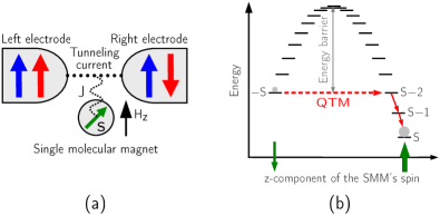
Figure 1: (color online) (a) Schema of the system under consideration for parallel (black solid arrows) and antiparallel (grey solid arrows) magnetic configurations. (b) Energy levels corresponding to different spin states of the SMM. The grey dots represent the occupancy of the molecular spin states when the third resonant field is reached.

Theoretical description In a recent paper Misiorny06 we considered the situation when a bias voltage was applied between the two external ferromagnetic leads, and the spin reversal was due to the associated spin current. Here, we consider a different situation, i.e. the system is unbiased but instead an external magnetic field is applied to switch the molecule owing to the QTM phenomenon. The switching is accompanied by a current impulse between the leads, which is a consequence of the spin relaxation processes. This, in turn, is associated with transfer of a certain charge between the leads.

The simplest model Hamiltonian describing the SMM takes the form vanHammen-SutoEurphysLett1/86 ; Dobrovitsky-ZvezdinEurophysLett38/97 ; Wernsdorfer-SessoliScience284/99

$$\mathcal{H}_{S\!M\!M}=\mathcal{H}_{0}+\mathcal{H}_{QT\!M}+\mathcal{H}_{I}.$$ (1)

The first term includes the uniaxial anisotropy and the Zeeman energy of the molecule in a field along the anisotropy axis (the field varies linearly in time),

$$\mathcal{H}_{0}=-DS_{z}^{2}+g\mu_{B}S_{z}H_{z},$$ (2)

where $S_{z}$ is the $z$-component of the spin operator, $D$ is the uniaxial magnetic anisotropy constant, $g$ is the Landé factor, and $\mu_{B}$ stands for the Bohr magneton.

The next term, $\mathcal{H}_{QT\!M}$, of the Hamiltonian is involved in the phenomenon of QTM, and includes the transverse anisotropy and the Zeeman energy of the molecule in a field perpendicular to the anisotropy axis,

$$\mathcal{H}_{QT\!M} =E(S_{x}^{2}-S_{y}^{2})+C(S_{+}^{4}+S_{-}^{4})$$

$$+g\mu_{B}(S_{x}H_{x}+S_{y}H_{y}),$$ (3)

where $S_{x}$ and $S_{y}$ are the transverse components of the spin operator, $S_{\pm}=S_{x}\pm\imath S_{y}$, whereas $E$ and $C$ are the transverse magnetic anisotropy constants. The perpendicular magnetic field is much weaker than the longitudinal component $H_{z}$, and is assumed to grow in time with the same time scale as $H_{z}$, i.e. $H_{x}=0.1H_{z}$ ($H_{y}=0$ for simplicity).

The last term of the Hamiltonian, $\mathcal{H}_{I}$, describes exchange interaction between electrons of both leads and the SMM AppelbaumPRL17/66 ; AppelbaumPR154/67 ; KimPRL92/04 ,

$$\mathcal{H}_{I}=\frac{1}{2}\sum_{q,q^{\prime}}\sum_{{\bf k}{\bf k}^{\prime}\alpha\beta}\frac{J_{q,q^{\prime}}}{\sqrt{N_{q}\,N_{q^{\prime}}}}\>\bm{\sigma}_{\alpha\beta}\cdot\mathbf{S}\>a_{{\bf k}\alpha}^{q{\dagger}}a_{{\bf k}^{\prime}\beta}^{q^{\prime}}\ \>+\>\textrm{H.c.}.$$ (4)

Here, $\mathbf{S}$ is the SMM’s spin operator, $\bm{\sigma}=(\sigma^{x},\sigma^{y},\sigma^{z})$ is the Pauli spin operator for conduction electrons, $a^{q}_{{\bf k}\alpha}$ ($a^{q{\dagger}}_{{\bf k}\alpha}$) are the annihilation (creation) operators of electrons in the left ($q=L$) or right ($q=R$) electrodes, ${\bf k}\ ({\bf k^{\prime}})$ denotes a wave vector, and $\alpha\ (\beta)$ is the electron spin index. In eq. (4) $J_{q,q^{\prime}}$ is the relevant exchange parameter, assumed to be independent of energy and polarization of the leads. In a general case $J_{L,L}\neq J_{R,R}\neq J_{L,R}=J_{R,L}$. In the following, however, we assume the symmetrical situation, where $J_{L,L}=J_{R,R}=J_{L,R}=J_{R,L}\equiv J$. Owing to the proper normalization, $J$ is also independent of the electodes’ size. Finally, in eq. (4) $N_{q}$ ($q=L,R$) denotes the number of elementary cells in the $q$-th electrode. Since we consider only the unbiased situation, we have omitted the direct tunneling between the leads (i.e., tunneling without exchange interaction with the molecule).

First, we present some general equations describing spin relaxation of the molecule, and start from the transition rates $\gamma_{m}^{>(<)}=\gamma_{m}^{L\!R\,>(<)}+\gamma_{m}^{R\!L\,>(<)}+\gamma_{m}^{L\!L\,>(<)}+\gamma_{m}^{R\!R\,>(<)}$, at which the molecule’s spin changes from $|m\rangle$ to the upper (lower) state $|m\pm 1\rangle$ due to coupling to the leads. Here, $\gamma_{m}^{L\!R\,>(<)}$ is the transition rate of electrons tunneling from the left to right electrode, whereas $\gamma_{m}^{R\!L\,>(<)}$ corresponds to electrons tunneling the other way. Similar meaning have the rates $\gamma_{m}^{L\!L\,>(<)}$ and $\gamma_{m}^{R\!R\,>(<)}$. They refer, however, to electrons which when interacting with the molecule change its magnetic state, but remain in the same electrode. All these transition rates can be calculated from the Fermi golden rule, and for instance

$$\gamma_{m}^{L\!R\,>(<)}=\sum_{{\bf k}\alpha}\sum_{{\bf k^{\prime}}\beta}W^{L{\bf k}\alpha m}_{R{\bf k}^{\prime}\beta m\pm 1}\>f(\epsilon_{{\bf k}\alpha}^{L})\left[1-f(\epsilon_{{\bf k}^{\prime}\beta}^{R})\right],$$ (5)

where $f(\epsilon)$ is the Fermi–Dirac distribution, and $\epsilon_{{\bf k}\alpha}^{q}$ ($q=L,R$) is the energy of electron states in the leads. The probability of electron transitions from the initial state $i\leftrightarrow\{L{\bf k}\alpha m\}$ to the final one $j\leftrightarrow\{R{\bf k}^{\prime}\beta m\pm 1\}$ is given by $W^{i}_{j}=(2\pi/\hbar)|\langle j|\mathcal{H}_{I}|i\rangle|^{2}\delta(E_{j}-E_{i})$, where $E_{i}=\epsilon_{{\bf k}\alpha}^{L}+E_{m}$, and $E_{m}$ is the energy of the unperturbed molecular spin state $|m\rangle$. Energy $E_{j}$ of the final state is given by a similar expression. Finally, similar formulae also hold for the transition rates $\gamma_{m}^{R\!L\,>(<)}$, $\gamma_{m}^{L\!L\,>(<)}$ and $\gamma_{m}^{R\!R\,>(<)}$.

The final expressions for the transition rates $\gamma_{m}^{>(<)}$ are given by the formulae

$$\gamma_{m}^{>(<)} =\frac{2\pi}{\hbar}|J|^{2}A_{\pm}(m)$$

$$\hskip 11.38092pt\times\Big{\{}D_{\uparrow}^{L}D_{\downarrow}^{R}+D_{\downarrow}^{L}D_{\uparrow}^{R}+D_{\uparrow}^{L}D_{\downarrow}^{L}+D_{\uparrow}^{R}D_{\downarrow}^{R}\Big{\}}$$

$$\hskip 11.38092pt\times\zeta\Big{(}\pm D(2m+1)\mp g\mu_{B}H_{z}\Big{)},$$ (6)

where $D_{\sigma}^{q}$ is the density of states (DOS) at the Fermi level in the $q$-th electrode for spin $\sigma$, $A_{\pm}(m)$ is defined as $A_{\pm}(m)=S(S+1)-m(m\pm 1)$, and $\zeta(\epsilon)=\epsilon\big{[}1-\exp(-\epsilon\beta)\big{]}^{-1}$ with $\beta^{-1}=k_{B}T$.

Since our objective is to calculate the average value of the $z$ component of SMM’s spin, $\langle S_{z}\rangle=\sum_{m}mP_{m}$, we have to determine the probabilities $P_{m}$ of finding the SMM in the spin state $|m\rangle$. To start with, we assume the initial spin state of the SMM to be $|-S\rangle$. Taking into account negative sign of the gyromagnetic factor, we write $H_{z}=-H$. Thus, in the initial state the magnetic field $H$ is negative. The field $H$ grows then linearly in time and the SMM’s spin undergoes transitions (due to QTM) at relevant resonant fields from the state $|-S\rangle$ to states $|S-M\rangle$ (consecutively for $M=0$, $M=1$, etc) on the opposite side of the energy barrier. The probabilities of all other states (for each $M$), i.e. of states $|-S+1\rangle,\ldots,|S-M-1\rangle$, are then equal to zero. If the SMM’s spin tunnels to the state other than $|S\rangle$, the interaction of the molecule with the electron reservoirs leads to further relaxation of the spin to the final state $|S\rangle$, fig. 1(b).

There are two time scales set respectively by the speed $c$ at which the magnetic field is increased, $c=dH/dt$, and the relaxation processes due to interaction with the electrodes, with the latter scale being much shorter. This fact can be used to simplify the problem, and the probabilities $P_{m}$ can be then found from the set of master equations, separately for each field range between the successive resonant fields at which the QTM occurs. Moreover, when $T\ll D$, the relevant relaxation processes are those which lower energy of the molecule (and increase the quantum number $m$ in the case under consideration). For the $M$-th range the equations take then the form

$$\left\{\begin{aligned} c\,\dot{P}_{S-M}&\>=\>-\>\gamma_{S-M}^{>}P_{S-M},\\ c\,\dot{P}_{m}&\>=\>-\>\gamma_{m}^{>}P_{m}\>+\>\gamma_{m-1}^{>}P_{m-1},\\ c\,\dot{P}_{S}&\>=\>\gamma_{S-1}^{>}P_{S-1},\end{aligned}\right.$$ (7)

for $m\in\langle S-M+1,S-1\rangle$, and $\dot{P}$ defined as $\dot{P}\equiv dP/dH$. One should bear in mind that the transition rates $\gamma_{m}^{>}$ depend on magnetic field (see eq. (Quantum tunneling of magnetization in single molecular magnets coupled to ferromagnetic reservoirs)). Additionally, we note that $\gamma_{m}^{<}\approx 0$ for $m\geq 1$, which justifies the absence of terms corresponding to the transitions to lower molecular spin states in eqs. (7).

The boundary conditions for the probabilities in eqs. (7) (at the resonant field $H^{(M)}$) are:

$$\left\{\begin{aligned} P_{S-M}\Big{(}H^{(M)}\Big{)}&\>=\>\widetilde{P}_{S-M},\\ P_{m}\Big{(}H^{(M)}\Big{)}&\>=\>P_{m}^{M-1}\Big{(}H^{(M)}\Big{)}\\ \end{aligned}\right.$$ (8)

for $m\in\langle S-M+1,S\rangle$. In eqs. (8) $P_{m}^{n}\big{(}H^{(n+1)}\big{)}$ denotes the probability $P_{m}$ calculated for the field range $\langle H^{(n)},H^{(n+1)}\rangle$ and taken at the field $H^{(n+1)}$. Moreover, $\widetilde{P}_{S-n}$ is the probability of the QTM to occur between the states $|-S\rangle$ and $|S-n\rangle$. This probability can be obtained analytically with the repetitive use of the two-level Landau-Zener model KimPRL92/04 ; ZenerPRSL32/137 , $\widetilde{P}_{S-n}=\big{(}1-\exp[-2\pi\lambda_{n}]\big{)}\prod_{l=0}^{n-1}\exp[-2\pi\lambda_{l}]$, where $\lambda_{n}=\Delta_{n}^{2}/\big{[}4\hbar(2S-n)g\mu_{B}c\big{]}$ and $\Delta_{n}$ is the splitting of the two states due to the $\mathcal{H}_{QT\!M}$ term in Hamiltonian.

Numerical results Numerical calculations have been obtained for an octanuclear iron(III) oxo-hydroxo cluster of the formula $\left[\textrm{Fe}_{8}\textrm{O}_{2}(\textrm{OH})_{12}(\textrm{tacn})_{6}\right]^{8+}$ (shortly $\textrm{Fe}_{8}$), whose total spin number is $S=10$. The anizotropy constants $D=0.292$ K, $E=0.046$ K, $C=-2.9\times 10^{-5}$ K as well as the splittings $\Delta_{n}$ are adopted from refs. Wernsdorfer-SessoliScience284/99 ; Rastelli-TassiPRL64/01 . We assume that $J\approx 100$ meV. Furthermore, for both leads we assume the elementary cells are occupied by 2 atoms contributing 2 electrons each. The density of free electrons is assumed to be $n\approx 10^{29}m^{-3}$. The electrodes are characterized by the polarization parameter $P^{q}=(D_{+}^{q}\>-\>D_{-}^{q})/(D_{+}^{q}\>+\>D_{-}^{q})$, where $D_{+(-)}^{q}$ denotes the DOS of majority (minority) electrons in the $q$-th electrode. The temperature of the system is assumed to be $T=0.01$ K, which is below the blocking temperature $T_{B}=0.36$ K of $\textrm{Fe}_{8}$.

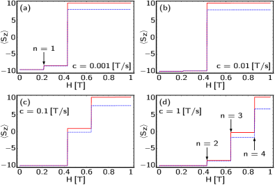
Figure 2: (color online) The average value of the SMM’s spin, $\langle S_{z}\rangle$, as a function of external magnetic field $H$ for various field sweeping speeds $c$. The magnetic moments of the electrodes are in the parallel configuration and $P^{L}=P^{R}=0.5$. Solid lines represent the case of the SMM’s spin coupled to electrons, whereas dashed ones describe the system without the exchange interaction between the molecule and electrons (and in the absence of other spin relaxation processes).

Let us consider first the average value of the z component of SMM’s spin, $\langle S_{z}\rangle$, in an external magnetic field increasing linearly in time, fig. 2. The reversal of the SMM’s spin is due to the QTM, whose signature is the characteristic staircase pattern. The steps occur at the resonant fields where the QTM is allowed, and their heights are determined by the field sweeping speed $c$ and parameters of the $\mathcal{H}_{QT\!M}$ term. For small values of $c$ full reversal occurs already at the third resonance field (corresponding to $n=2$). The exchange coupling with reservoirs is essential to observe the full reversal of the spin – after QTM the spin relaxes to the state $|S\rangle$.

Typical values of the transition times $1/\gamma_{m}^{>}$ (for the parameters assumed) are of the order of $10^{-13}-10^{-12}$ s. The duration of the SMM’s spin reversal is thus set by the rate $c$ at which the field $H$ is augmented, and it varies between $1$ s, fig. 2(d), and $10^{3}$ s, fig 2(a). As a consequence, the steps in figs. 2 are very sharp.

Generally, the values of $\gamma_{m}^{>}$ depend on the magnetic configuration of the system. Assume the same total density of states in both electrodes, but generally different spin polarizations. In the parallel (P) configuration $\gamma_{m}^{P\,>}\propto 1-(P^{L}+P^{R})^{2}/4$, whereas in the antiparallel (AP) one $\gamma_{m}^{A\!P\,>}\propto 1-(P^{L}-P^{R})^{2}/4$. If additionally we assume now $P^{L}=P^{R}\equiv P$, the above formulae reduce to $\gamma_{m}^{P\,>}\propto 1-P^{2}$ for the parallel configuration, while in the antiparallel configuration $\gamma_{m}^{A\!P\,>}$ is independent on the polarization $P$. The difference between these two configurations can be clearly seen for $P=1$, which corresponds to the situation with both electrodes being perfect halfmetallic ferromagnets. In this limiting situation $\gamma_{m}^{P\,>}\rightarrow 0$ while $\gamma_{m}^{A\!P\,>}$ is nonzero and independent of $P$.

The quantum tunneling phenomenon leads to another interesting feature of the system under consideration. Generally, variation of the $S_{z}$ component of the SMM’s spin by one is associated with spin reversal of one of the electrons in the leads. In the considered situation, an electron flips its spin from $\uparrow$ to $\downarrow$, which is accompanied by the transition of the molecule state from $|m\rangle$ to $|m+1\rangle$. This process is continued until the probability of finding the SMM in the spin state $|S\rangle$ is equal to 1, which corresponds to full reversal of the SMM’s spin. Moreover, some of the spin-flip relaxation processes are associated with a transfer of a single electron charge from one electrode to the other. Owing to the spin asymmetry, the average charge transferred between the leads during magnetic moment switching becomes nonzero. As a consequence, one can expect a current pulse ($I_{r}$) associated with the spin relaxation after crossing each resonant magnetic field Elste06a . The general formula for the relaxation current flowing from the left to right side of the junction is $I_{r}=e\sum_{j=1}^{M}\sum_{m=1}^{j}P_{S-m}\big{(}\gamma_{S-m}^{R\!L\,>}-\gamma_{S-m}^{L\!R\,>}\big{)}$, where $e$ is the electron charge, and $P_{S-m}$ as well as $\gamma_{S-m}^{R\!L(L\!R)\,>}$ depend on the field $H$. Here, $M$ is determined from the condition $\widetilde{P}_{S-(M+1)}\approx 0$. The time scale on which relaxation currents vanish is of the order of the relaxation times. For these reasons, current impulses are very short for the parameters corresponding to fig. 2 and would not be resolved.

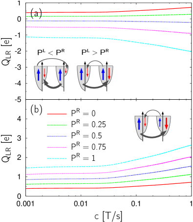
Figure 3: (color online) The average charge $Q_{L\!R}$ transferred between the electrodes during the SMM’s spin reversal process as a function of the field sweeping speed $c$ for various polarizations of the right electrode $P^{R}$. The polarization of the left electrode is $P^{L}=0.4$. The magnetic moments of the leads are kept either in the parallel (a) or in the antiparallel (b) configuration. The insets represent the DOS at the Fermi level in the leads, where the arrows indicate the direction of the charge transfer between the leads.

We note that the transition times only slightly change when the field is increased, and the corresponding time scale is considerably smaller than the time scale set by $c$. Therefore one can assume that they are constant, which allows us to find analytic expression for the total electronic charge transferred from the left to the right lead during the reversal of the SMM’s spin, $Q_{L\!R}=e\Gamma\sum_{j=1}^{M}j\widetilde{P}_{S-j}$, see figs. 3. $\Gamma$ is a coefficient whose value depends on the magnetic configuration of the leads, and $\Gamma_{A\!P(P)}=2(P^{L}\pm P^{R})/[4-(P^{L}\mp P^{R})^{2}]$, respectively for the parallel (lower sign) and antiparallel (upper sign) magnetic configurations.

The sign of $Q_{LR}$, which is related to the direction of average charge flow, is determined by the magnetic configuration of the system. In the antiparallel configuration we observe only one direction of the average charge flow, i.e. from left to right. In the parallel configuration, on the other hand, the average flow can be either from left to right ($P^{L}>P^{R}$) or from right to left ($P^{R}>P^{L}$). For $P^{L}=P^{R}$ there is no resultant flow of charge. The change of the charge transfer direction can be explained by considering the DOS at the Fermi level in both electrodes and taking into account that a change in the SMM’s spin state is possible only when it is associated with the flip of an electron from $\uparrow$ to $\downarrow$.

In conclusions, we have considered spin reversal of a SMM due to the phenomenon of QTM in a time dependent magnetic field and in the presence of two external spin-polarized leads. The molecule was assumed to be coupled to electrons in both leads via exchange coupling. We showed that full spin reversal is associated with a transfer of certain charge from one lead to the other, despite no bias voltage is applied. When external bias is applied, then new effects may be observed Heersche06 ; Jo06 ; Leuenberger06 ; Romeike06 .

Acknowledgements This work is partly supported by funds of the Polish Ministry of Science and Higher Education as a research project in years 2006-2009.

References

- (1) R. Sessoli, D. Gatteschi, A. Caneschi and M.A. Novak, Nature(London) 365, 141 (1993).
- (2) D. Gatteschi and R. Sessoli, Angew. Chem. Int. Ed. 42, 268 (2003).
- (3) M. Misiorny and J. Barnaś, Phys. Rev. B 75, 134425 (2007).
- (4) F. Elste and C. Timm, cond-mat/0611108 (to be published in Phys. Rev. B).
- (5) C. Joachim, J.K. Gimzewski and A. Aviram, Nature 408, 541 (2000).
- (6) C. Timm and F. Elste, Phys. Rev. B 73, 235304 (2006).
- (7) E. M. Chudnovsky and J. Tejada, Macroscopic Quantum Tunneling of the Magnetic Moment (Cambridge University Press, 1998).
- (8) L.Thomas et al., Nature(London) 383, 145 (1996).
- (9) J. L. van Hemmen and A. Sütő, Europhys. Lett. 1 (10), 481 (1986).
- (10) V. V. Dobrovitsky and A. K. Zvezdin, Europhys. Lett. 38 (5), 377 (1997).
- (11) W. Wernsdorfer and R. Sessoli, Science 284, 133 (1999).
- (12) J. Appelbaum, Phys. Rev. Lett. 17, 91 (1966).
- (13) J. Appelbaum, Phys. Rev. 154, 633 (1967).
- (14) G.-H. Kim and T.-S. Kim, Phys. Rev. Lett. 92, 137203 (2004).
- (15) C. Zener, Proc. R. Soc. London, Ser. A 137, 696 (1932).
- (16) E. Rastelli and A. Tassi, Phys. Rev. B 64, 64410 (2001).
- (17) F. Elste and C. Timm, Phys. Rev. B 73, 235305 (2006).
- (18) H.B. Heersche, Z. de Groot, J.A. Folk, and H.S.J. van der Zant et al., Phys. Rev. Lett. 96, 206801 (2006).
- (19) M.-H. Jo et al., Nano Lett. 6, 2014 (2006).
- (20) M.N. Leuenberger and E.R. Mucciolo, Phys. Rev. Lett. 97, 126601 (2006).
- (21) C. Romeike, M.R. Wegewijs, W. Hofstetter, and H. Schoeller, Phys. Rev. Lett. 96, 196601 (2006).