A supercritical series analysis for the generalized contact process with diffusion

Abstract

We study a model that generalizes the CP with diffusion. An additional transition is included in the model so that at a particular point of its phase diagram a crossover from the directed percolation to the compact directed percolation class will happen. We are particularly interested in the effect of diffusion on the properties of the crossover between the universality classes. To address this point, we develop a supercritical series expansion for the ultimate survival probability and analyse this series using d-log Padé and partial differential approximants. We also obtain approximate solutions in the one- and two-site dynamical mean-field approximations. We find evidences that, at variance to what happens in mean-field approximations, the crossover exponent remains close to $\phi=2$ even for quite high diffusion rates, and therefore the critical line in the neighborhood of the multicritical point apparently does not reproduce the mean-field result (which leads to $\phi=0$) as the diffusion rate grows without bound.

1 Introduction

Phase transitions in stochastic models have attracted a great attention in recent years. Although much work has been done on systems whose stationary states are described by thermodynamics, also phase transitions in systems far from equilibrium have been studied in much detail, and it is remarkable that concepts of scaling and universality, developed in the context of thermodynamic phase transitions, have been applied successfully in these new situations as well. In particular, systems which exhibit absorbing states, and therefore do not obey detailed balance, are a rich group of models where out of equilibrium phase transitions have been studied. Much of this work has been done based on numerical simulations, stochastic models are very well fitted to these techniques, but analytical approaches are also useful and may sometimes lead to very precise results. Therefore, as in other fields of Physics, simulational and analytical approaches are complementary to study non-equilibrium phase transitions [1].

One of the largest and most studied universality classes in models with absorbing states is the directed percolation (DP) class, and in this class the most studied model is the contact process (CP), which in one of his interpretations was formulated as a very simple model to describe the evolution of an epidemic disease, which spreads through contact between healthy and sick individuals, placed on sites of a lattice. In this model, at each site of the lattice an individual is located, and this individual will be in one of two states: healthy or sick. It is usual to associate a sick individual to a particle and a healthy one to a hole. Particles are created autocatalytically, that is, a particle may be created at an empty site with a rate which is proportional to the number of occupied first neighbor sites of this site. An occupied site may become empty with a unitary rate (spontaneous healing). Even in one dimension, a phase transition is found in the model between the absorbing stationary state (in which all individuals are healthy and no new sick person may be generated by contact, or else for a lattice without any particle) and a stationary phase with a nonzero fraction of particles, called active state [2]. The contact process is related to several other stochastic models [3, 4, 5, 6], and the directed percolation universality class seems to include all models where a transition between an absorbing and an active state occurs, with a scalar order parameter, short range interactions and no conservation laws [7]. No exceptions to this conjecture have been reported so far [8].

Recently, a generalization of the CP was studied using mean-field approximations and simulations [9], as well as series expansions [10]. In this model, an additional process is included besides the autocatalytic creation and the spontaneous annihilation of particles: the autocatalytic creation of holes, that is, an occupied site may become empty by two processes: either spontaneously or with a rate which is proportional to the number of empty first neighbor sites. It is more natural to describe this model in terms of two distinct types of particles, $A$ and $B$, requiring that each lattice site at any time is either occupied by an $A$ or a $B$ particle. The process $B\to A$ occurs with a rate which is proportional to the number of first neighbor sites with $A$ particles, whereas the opposite process $A\to B$ may happen either spontaneously or with a rate proportional to the number of first neighbor sites occupied by $B$ particles. The CP is a particular case of this model where no autocatalytic creation of $B$ particles is allowed. In another particular case, an additional symmetry is present in the model: when the spontaneous creation of $B$ particles is suppressed, the model becomes symmetric with respect to the interchange of $A$ and $B$ particles for equal creation rates of $A$ and $B$ particles, being known as the biased voter model [11], with a transition between two symmetric absorbing states, where the lattice is totally filled with the same type of particle. If the rates of the two processes ($A\to B$ and $B\to A$) are the same, the density of $A$ and $B$ particles does not change as the system evolves, but if the rate of one of these processes is larger, the system will reach the absorbing state in which only the particles created at a larger rate are present. This model, having an additional symmetry, belongs to the compact directed percolation (CDP) class, with critical exponents which are different from the ones found in the CP. The crossover between both universality classes was the major motivation to study this generalized model. In particular, the results of a two-variable series expansion for the ultimate survival probability of the model lead to rather precise evidences that the crossover exponent at the point where the universality class of the model changes is given by $\phi=2$, coincident with the mean-field value, which agrees both with the limits obtained by Liggett [12] and with simulational results [13] for the same crossover in the Domany-Kinzel automaton [14], thus providing an evidence that the process of update (parallel in the DK automaton and sequential in the CP) does not change the value of the crossover exponent.

It is of interest to study the effect of diffusion on the behavior of such models. This was already done for the CP, with the result that the transition point becomes a critical line as the new variable (rate of diffusion) is introduced in the model [15, 16]. In this case, as expected, mean-field results are obtained in the limit where the evolution of the system is dominated by diffusion, both in the values of the transition rate and of critical exponents. Thus the limit of infinite diffusion rate may also be viewed as a crossover transition between non-classical and classical behavior. These results may be heuristically justified if we note that in this limit, since diffusion processes are much more probable that the others, for each other process the local densities may be replaced by the global ones, eliminating the effect of fluctuations.

In this work we include diffusion in the generalized CP model described above, in order to find out its effect on the phase diagram and critical exponents of the model. After defining the model more precisely in section 2, we obtain its phase diagram in the two-site cluster mean-field approximation in section 3. We then proceed obtaining supercritical series expansions for the survival probability in section 4, which are analysed using Padé approximants and two-variable partial differential approximants in section 5. Conclusions and final comments may be found in section 6.

2 Definition of the model

The model is defined on a one-dimensional lattice with $N$ sites and periodic boundary conditions. Each site is occupied either by a particle $A$ or a particle $B$, no holes are allowed. The microscopic state of the model may thus be described by the set of binary variables $\eta=(\eta_{1},\eta_{2},\ldots,\eta_{N})$, where $\eta_{i}=0$ or $1$ if site $i$ is occupied by particles $B$ or $A$, respectively.

The model evolves in time according to the following Markovian rules:

1. A site $i$ of the lattice is chosen at random.

2. If the site is occupied by a particle B, it becomes occupied by a particle A with a transition rate equal to $p_{a}n_{A}/2$, where $n_{A}$ is the number of A particles in the sites which are first neighbors to site $i$.

   $$\framebox{A}\mbox{ }B\mbox{ }\framebox{B}\stackrel{{\scriptstyle\tiny{p_{a}/2}}}{{\longrightarrow}}\framebox{A}\mbox{ }A\mbox{ }\framebox{B}$$

3. If site $i$ is occupied by a particle A, it may become occupied by a particle B through three processes:

   • Spontaneously, with a transition rate $p_{c}$.

     $$A\stackrel{{\scriptstyle\tiny{p_{c}}}}{{\longrightarrow}}B$$

   • Through an autocatalytic reaction, with a rate $p_{b}n_{B}/2$, where $n_{B}$ is the number of B particles in the sites which are first neighbors to site $i$.

     $$\framebox{A}\mbox{ }A\mbox{ }\framebox{B}\stackrel{{\scriptstyle\tiny{p_{b}/2}}}{{\longrightarrow}}\framebox{A}\mbox{ }B\mbox{ }\framebox{B}$$

   • By interchanging the $B$ particle with an $A$ particle located in a first neighbor site to site $i$. This transition occurs with rate equal $\tilde{D}$.

     $${}A\mbox{ }\framebox{B}\stackrel{{\scriptstyle\tiny{\tilde{D}}}}{{\longrightarrow}}B\mbox{ }\framebox{A}$$

   where indicates the state of the first neighbour.

We define the time in such a way the the non-negative rates $p_{a}$, $p_{b}$, and $p_{c}$ obey the normalization $p_{a}+p_{b}+p_{c}=1$. We may then discuss the behavior of the model in the $(p_{a},p_{c},\tilde{D})$ space without loss of generality.

When $p_{c}\neq 0$ the configuration where all the sites are occupied by particles $B$ is absorbing, while for $p_{c}=0$ both symmetrical configurations in which all sites are occupied by the same particles are absorbing, independently of the value of $\tilde{D}$. In the particular case $p_{b}=0$, in which the model corresponds to the CP with diffusion, there exists a critical line in the $(p_{a},p_{b},\tilde{D})$ space where an active configuration (with nonzero density of $A$ particles) becomes identical with the absorbing one. This line becomes a critical surface in the general case $p_{b}\neq 0$. Based on the symmetries of the model this surface must be of second order with critical exponents of DP class for finite values of the diffusion rate $\tilde{D}$, except for the case $p_{c}=0$. In this case, the transition occurs between two absorbing states (lattice full by particles $A$ or $B$) at the the point $p_{a}=1/2$, $\forall\tilde{D}$, with critical exponents of the CDP class.

For a certain fixed value of $\tilde{D}$, the behavior of any stationary density close to multicritical point $(p_{a}=1/2,p_{c}=0)$ should exhibit the scaling form,

$$g(p_{a}-1/2,p_{c},\tilde{D})\sim(p_{a}-1/2)^{e_{g}(\tilde{D})}F\left(\frac{p_{c}}{|p_{a}-1/2|^{\phi(\tilde{D})}}\right).$$ (1)

The critical exponent associated with the density variable $g$, $e_{g}(\tilde{D})$, should correspond to the CDP universality class, and the scaling function $F(z)$ is singular at a value $z_{0}(\tilde{D})$ of its argument, which corresponds to the critical line for a given value of $\tilde{D}$. Thus, the critical line is asymptotically given by $p_{c}=z_{0}(\tilde{D})(pa-1/2)^{\phi(\tilde{D})}$. In this way we have two exponents as a function of the diffusion and it is interesting to find out how the exponents change as diffusion processes are introduced in the model.

3 Cluster Approximations

We have derived solutions for the cluster dynamic approximations in simple mean-field (one-site) and two-site levels [1]. The simple mean-field solution is independent of the diffusion rate, and the critical line is located at $p_{a}=1/2$, independently of $p_{c}$. Thus, in this approximation the crossover exponent vanishes identically. The lowest order of mean-field cluster approximation in which the effect of diffusion is present in the results is the two-site approximation. Without going into the details of this approximation, since the calculations are similar to the ones performed recently in the model without diffusion [9], in the two-site level cluster approximation the critical line is given by:

$$p_{a}^{c}=\frac{1}{8}\left[4-(p_{c}+2\tilde{D})+\sqrt{(p_{c}+2\tilde{D})^{2}+8p_{c}}\right].$$ (2)

We notice that as the value of $\tilde{D}$ grows, the critical line approaches the result obtained in the one-site approximation, as expected. If we expand equation 2 for small values of $p_{c}$, we obtain $p_{a}^{c}-1/2\approx 2p_{c}/\tilde{D}$, showing that the two-site approximation leads to the crossover exponent $\phi=1$ for any finite value of the diffusion rate $\tilde{D}$ and $\phi=0$ in the limit of infinite diffusion rate. For vanishing diffusion rate, we obtain the crossover exponent $\phi=2$.

Another point which is worth noticing is the crossover as the diffusion rate approaches infinity, where mean-field behavior is expected. For this purpose, we may define the variables $\alpha=(1-p_{a})/p_{a}$ and $D_{eff}=\alpha\tilde{D}/(1+\alpha\tilde{D})$. Rewriting the expression for the critical condition 2 in terms of the variables $x=1-\alpha$, $y=1-D_{eff}$, and $p_{b}$, we obtain:

$$y=\frac{x(x-2)}{p_{b}x^{3}+(1-4p_{b})x^{2}+(5p_{b}-1)x+1-2p_{b}}.$$ (3)

It is apparent that, as long as $p_{b}<1/2$, we have $\tilde{\phi}=1$ for the crossover between the regimes of finite and infinite diffusion. In the particular case $p_{b}=0$, which corresponds to the CP, we recover two-site approximation results obtained before [16]. For the particular case $p_{b}=1/2$, which corresponds to the CDP limit, we have the solution $x=0$ for any value of $y$, so that the locus of the transition is not affected by the diffusion. These results are illustrated in figure 1.

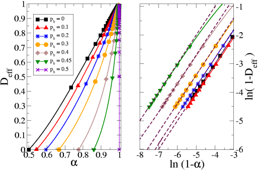
Figure 1: Results of the two-site approximation. In the left panel we see different phase diagrams for fixed values of $p_{b}$ using the new variables $\alpha$ and $D_{eff}$. In the right we have the estimates of the crossover exponent in each of these diagrams. In all cases the parallel dashed lines indicate that this exponent is $\tilde{\phi}=1$ for any value of the parameter $p_{b}<1/2$.

4 Derivation of the supercritical series for the model

Now let us develop a three-variable supercritical series expansion for the model. We follow closely the operator formalism presented in the paper by Jensen and Dickman on series for the CP process and related models [17]. We may represent the microscopic configurations of the lattice by the direct product of kets

$$|\eta\rangle=\bigotimes_{i}|\eta_{i}\rangle,$$ (4)

which are defined to be orthonormal

$$\langle\eta|\eta^{\prime}\rangle=\prod_{i}\delta_{\eta_{i},\eta_{i}\prime}.$$ (5)

Now we may define A particles creation and annihilation operators for the site $i$:

$$A_{i}^{\dagger}|\eta_{i}\rangle = (1-\eta_{i})|\eta_{i}+1\rangle,$$

$$A_{i}|\eta_{i}\rangle = \eta_{i}|\eta_{i}-1\rangle.$$ (6)

In this formalism, the state of the system at time $t$ may be represented as

$$|\psi(t)\rangle=\sum_{\{\eta\}}p(\eta,t)|\eta\rangle.$$ (7)

If we define the projection onto all possible states as

$$\langle\;|\equiv\sum_{\{\eta\}}\langle\eta|,$$ (8)

the normalization of the state of the system may be expressed as $\langle\;|\psi\rangle=1$. In this notation, the master equation for the evolution of the state of the system is

$$\frac{d|\psi(t)\rangle}{dt}=S|\psi(t)\rangle.$$ (9)

The evolution operator $S$ may be expressed in terms of the creation and annihilation operators as $S=\lambda R+V$ where

$$R = \sum_{i}[\gamma(2-A_{i-1}^{\dagger}A_{i-1}+A_{i+1}^{\dagger}A_{i+1})+1](A_{i}-A_{i}^{\dagger}A_{i})+$$ (10)

$$+ \bar{D}\sum_{i}(1-A_{i-1}^{\dagger}A_{i})A_{i-1}A_{i}^{\dagger}+(1-A_{i+1}^{\dagger}A_{i})A_{i+1}A_{i}^{\dagger},$$

$$V = \sum_{i}(A_{i}^{\dagger}+A_{i}^{\dagger}A_{i}-1)(A_{i-1}^{\dagger}A_{i-1}+A_{i+1}^{\dagger}A_{i+1}),$$ (11)

and the new parameters

$$\lambda\equiv\frac{2p_{c}}{p_{a}},$$

$$\gamma\equiv\frac{p_{b}}{2p_{c}}$$

and

$$\bar{D}\equiv\frac{\tilde{D}}{\lambda}$$

were introduced.

We notice that the operator $R$ includes the diffusion and the annihilation of A particles processes, while the creation of A particles is present in the operator $V$. Therefore, at small values of the parameter $\lambda$ creation of A particles is favored, and the decomposition above is convenient for a supercritical perturbation expansion. Let us show explicitly the effect of each operator on a generic configuration $(\mathcal{C})$.

$$R({\mathcal{C}}) = \gamma\sum_{i}({\mathcal{C}}^{\prime}_{i})+2\gamma\sum_{j}({\mathcal{C}}^{\prime}_{j})+\sum_{k}({\mathcal{C}}^{\prime}_{k})+$$ (12)

$$+ \bar{D}\left[\sum_{r}({\mathcal{C}}^{\prime\prime\prime}_{r})+\sum_{s}({\mathcal{C}}^{\prime\prime\prime r}_{s})+\sum_{t}({\mathcal{C}}^{\prime\prime\prime l}_{t})\right]+$$

$$- [\gamma(r_{1}+2r_{2})+\bar{D}(t_{1}+2t_{2})+r]({\mathcal{C}}),$$

where the first sum is over the $r_{1}$ sites with A particles and one B neighbor, the second sum is over the $r_{2}$ sites with A particles and two B neighbors, the third sum is over all $r$ sites with A particles of the configuration $(\mathcal{C})$. The next sum is again over the $r_{1}$ sites with A particles and one B neighbor and the two last sums are over the $r_{2}$ sites with A particles and two B neighbors. Configuration $({\mathcal{C}}_{i}^{\prime})$ is obtained replacing the A particle at site $i$ by a B particle, $({\mathcal{C}}^{\prime\prime\prime}_{i})$ is obtained interchanging the A particle at the site $i$ with its single B neighbor and finally, $({\mathcal{C}}^{\prime\prime\prime(r,l)}_{i})$ is a configuration where the A particle at the site $i$ is interchanged with the B particle located at the right ($r$) or to the left ($l$) of site $i$. It is convenient associate the diffusion with the annihilation process to avoid some ambiguity in truncating the series in a certain order. In the other hand, the action of operator $V$ is

$$V({\mathcal{C}})=\sum_{i}({\mathcal{C}}^{\prime\prime}_{i})+2\sum_{j}({\mathcal{C}}^{\prime\prime}_{j})-(q_{1}+2q_{2})({\mathcal{C}}),$$ (13)

where the first sum is over the $q_{1}$ sites with B particles and one A neighbor, the second sum is over the $q_{2}$ sites with B particles and two A neighbors. Configuration $({\mathcal{C}}_{i}^{\prime\prime})$ is obtained replacing the B particle at site $i$ in configuration $(\mathcal{C})$ by a A particle.

Since we are interested in the long time behavior of the system, it is useful to consider Laplace transforms. For the state ket we have:

$$|\tilde{\psi}(s)\rangle=\int_{0}^{\infty}e^{-st}|\psi(t)\rangle,$$ (14)

and inserting the formal solution $|\psi(t)\rangle=e^{St}|\psi(0)\rangle$ of the master equation 9, we find

$$|\tilde{\psi}(s)\rangle=(s-S)^{-1}|\psi(0)\rangle.$$ (15)

The stationary state $|\psi(\infty)\rangle\equiv\lim_{t\to\infty}|\psi(t)\rangle$ may then be found noticing that

$$|\psi(\infty)\rangle=\lim_{s\to 0}s|\tilde{\psi}(s)\rangle,$$ (16)

which may be obtained integrating 14 by parts. A perturbative expansion may be obtained assuming that $|\tilde{\psi}(s)\rangle$ may be expanded in powers of $\lambda$ and using 15,

$$|\tilde{\psi}(s)\rangle=|\tilde{\psi}_{0}\rangle+\lambda|\tilde{\psi}_{1}\rangle+\lambda^{2}|\tilde{\psi}_{2}\rangle+\cdots=\frac{1}{s-V-\lambda R}|\psi(0)\rangle.$$ (17)

Since

$$\frac{1}{s-V-\lambda R}=\frac{1}{s-V}\left[1+\lambda\frac{1}{s-V}R+\lambda^{2}\frac{1}{(s-V)^{2}}R^{2}+\cdots\right],$$ (18)

we arrive at

$$|\tilde{\psi}_{0}\rangle = \frac{1}{s-V}|\psi(0)\rangle$$

$$|\tilde{\psi}_{1}\rangle = \frac{1}{s-V}R|\tilde{\psi}_{0}\rangle$$ (19)

$$|\tilde{\psi}_{2}\rangle = \frac{1}{s-V}R|\tilde{\psi}_{1}\rangle$$ (20)

$$\vdots$$

The action of the operator $(s-V)^{-1}$ on an arbitrary configuration $({\mathcal{C}})$ may be found noting that

$$(s-V)^{-1}({\mathcal{C}})=s^{-1}({\mathcal{C}})+\frac{V}{s(s-V)}({\mathcal{C}}),$$ (21)

and using the expression 13 for the action of the operator $V$, we get

$$(s-V)^{-1}({\mathcal{C}})=s_{q}\left\{({\mathcal{C}})+(s-V)^{-1}\left[\sum_{i}({\mathcal{C}}^{\prime\prime}_{i})+2\sum_{j}({\mathcal{C}}^{\prime\prime}_{j})\right]\right\},$$ (22)

where the first sum is over the $q_{1}$ sites with B particles and one A neighbor, the second sum is over the $q_{2}$ sites with B particles and two A neighbors, and we define $s_{q}\equiv 1/(s+q)$, where $q=q_{1}+2q_{2}$.

It is convenient to adopt as the initial configuration a translational invariant one with a single A particle (periodic boundary conditions are chosen). Now we may notice in the recursive expression 22 that the operator $(s-V)^{-1}$ acting on any configuration generates an infinite set of configurations, and thus we are unable to calculate $|\tilde{\psi}\rangle$ in a closed form. We may, however, calculate the extinction probability $\tilde{p}(s)$, which corresponds to the coefficient of the vacuum state $|0\rangle$. As happens also for the models related to the CP studied in [17] configurations with more than $j$ particles only contribute at orders higher than $j$, and since we are interested in the ultimate survival probability for A particles $P_{\infty}=1-\lim_{s\to 0}s\tilde{p}(s)$, $s_{q}$ may be replaced by $1/q$ in Eq. 22. An illustration of this procedure may be seen in [10].

The algebraic operations above may be easily performed in a computer using a proper algorithm. The configurations are expressed as binary numbers and the coefficients as double precision variables. With rather modest computational resources (Athlon MP2200, double processor, 1Gb memory) it is not difficult to calculate the coefficients up to order 22. The required processing time amounts to about 2 hours, the limiting factor is actually the memory required for the calculation. We define the coefficients $b_{i,j,k}$ as:

$$P_{\infty}=1-\frac{1}{2}(2\gamma+1)\lambda-\frac{1}{4}(2\gamma+1)\lambda^{2}-\sum_{i=3}^{22}\sum_{j=0}^{i-1}\sum_{k=0}^{i-2}b_{i,j,k}\lambda^{i}\gamma^{j}\bar{D}^{k}.$$ (23)

The case $\alpha=0$ is leads to a series which is identical the the one for the CP with diffusion obtained in [15]. Also, for $\bar{D}=0$ the two-variable series for the model without diffusion is [10] is recovered. The set of coefficients is too large to be included here, but may be obtained upon request from the authors.

5 Analysis of the series

To obtain estimates of the critical properties of this model from the supercritical series for the ultimate survival probability, given by equation 23, we start by using the d-log Pad approximants approach. These approximants are defined as ratios of two polynomials

$$F_{LM}(\lambda)=\frac{P_{L}(\lambda)}{Q_{M}(\lambda)}=\frac{\sum_{i=0}^{L}p_{i}\lambda^{i}}{1+\sum_{j=1}^{M}q_{j}\lambda^{j}}=f(\lambda).$$ (24)

In our case the function $f(\lambda)$ represents the series for $\frac{d}{d\lambda}\ln P_{\infty}(\lambda)$, where we fix the two remaining parameters $\gamma$ and $\bar{D}$. Therefore, we may obtain approximants with $L+M\leq 22$, and since it is known that diagonal ($L=M$) and near-diagonal approximants usually exhibit better convergence properties, we restrict our calculations to the set of approximants such that $L=M+\theta$, with $\theta=0,\pm 1$. We built approximants for the values of $\gamma$ ranging between 0 and 45, using $D=\bar{D}/(1+\bar{D})=0,0.1,0.2,0.3,0.4,0.5,0.7,0.8$ and $0.85$. In the table 1 some estimates for the critical value of the parameter $\lambda$ are shown. The estimates poles are roots of the polynomial $Q_{M}$ (poles of the approximant).

D	$\gamma$	L	M	$\lambda_{c}$
0	0.2	10	10	0.49472
		11	11	0.49472
0.1	0.2	10	10	0.50476
		11	11	0.50476
0.7	0.2	10	10	0.64708
		11	11	0.64750
0.8	0.2	10	10	0.75146
		11	11	0.71941

Table 1: Examples of estimates for critical points obtained by d-log Pad approximants. Notice that as the value of $D=\bar{D}/(1+\bar{D})$ grows the dispersion in the estimates obtained from different approximants for this critical point also grows.

With the data provided by the set of approximants, we obtained the critical lines using the original variables $p_{a}$ and $p_{c}$, for different values of the diffusion rate $\bar{D}$. Each point of these curves, shown in the figure 2, was calculated as the average of the estimates provided by the set of approximants, and the error bar associated to it corresponds to the standard deviation of the estimates. As the diffusion rate increases, the dispersion of the approximants also grows and the precision of the result becomes smaller generating relatively higher errors. Even so, it is possible to notice that all the critical curves approach of the multicritical point with a quadratic curvature, and thus the present results are different from the ones provided in the mean-field two-sites approximation shown above, which lead to $\phi=1$.

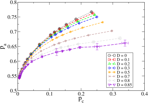
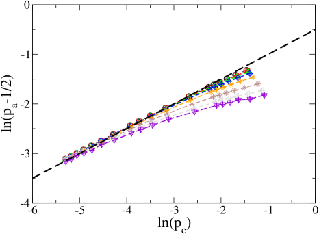
Figure 2: It the top panel we see the phase diagrams of the model obtained from d-log Pad approximants for several values of the diffusion rate $D=\bar{D}/(1+\bar{D})$. The graph in the bottom shows log-log plot of the same curves with the dashed line indicating the value of $\phi^{-1}=1/2$.

The critical exponent $\beta$ associated to the order parameter also can be estimated from the d-log Pad approximants, calculating the residue associated to the physical pole of each approximant. In the figure 3, the average values of the estimates for $\beta$ are depicted for different values of the diffusion rate. They are consistent with the conjecture that the value of the DP universality class $\beta_{DP}=0.276486(8)$ [18] applies to the model with finite rates of diffusion. Also, as expected, we notice that the dispersion of the estimates grows as the CDP point is approached ($p_{c}\to 0$)

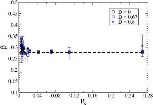
Figure 3: Behavior of the exponent $\beta$ as a function of the parameter $p_{c}$ for three different values of the diffusion rate. The value corresponding to the DP universality class is shown as a dashed line.

The behavior of the model in the limit of infinite diffusion rate is out of the reach of this analysis, partially because the reduction of the series to a variable leads to poor results in the neighborhood of a multicritical point, as is known of other similar cases [19] and therefore the d-log Pad approximants suffer great fluctuations in the region of high diffusion, as already found in the model without diffusion [10].

In an attempt to improve the series analysis we may use the Partial Differential Approximants (PDA’ s), which are appropriate for the study of two-variables series of models which undergo multicritical phenomena [19]. They may be regarded as a generalization to two variables of the d-log Padé approximants. The defining equation of the approximants is

$$P_{\mathbf{L}}(x,y)F(x,y)=Q_{\mathbf{M}}(x,y)\frac{\partial F(x,y)}{\partial x}+R_{\mathbf{N}}(x,y)\frac{\partial F(x,y)}{\partial y},$$ (25)

where $P$, $Q$, and $R$ are polynomials in the variables $x$ and $y$ with the set of nonzero coefficients ${\mathbf{L}}$, ${\mathbf{M}}$, and ${\mathbf{N}}$, respectively. The coefficients of the polynomials are obtained through substitution of the series expansion for the quantity which is going to be analyzed

$$f(x,y)=\sum_{k,k^{\prime}=0}f(k,k^{\prime})x^{k}y^{k^{\prime}}$$ (26)

into the defining equation 25 and requiring the equality to hold for a set of indexes defined as ${\mathbf{K}}$. The coefficients of the polynomials are then found solving a set of linear equations. Since the coefficients $f_{k,k^{\prime}}$ of the series are known for a finite set of indexes this sets an upper limit to the number of coefficients in the polynomials. The number of equations has to match the number of unknown coefficients, and thus $K=L+M+N-1$ (as in the Padé approximants, one coefficient is fixed arbitrarily). An additional issue, which is not present in the one-variable case, is the symmetry of the polynomials. Two frequently used options are the triangular and the rectangular arrays of coefficients. The choice of these symmetries is related to the symmetry of the series itself [20].

Let us suppose that the quantity represented by the series is expected to have a multicritical behavior at a point $(x_{c},y_{c})$, described by the scaling behavior:

$$f(x,y)\approx|\Delta\widetilde{x}|^{-e_{f}}Z\left(\frac{|\Delta\widetilde{y}|}{|\Delta\widetilde{x}|^{\phi}}\right),$$ (27)

where

$$\Delta\widetilde{x}=(x-x_{c})-(y-y_{c})/e_{2},$$ (28)

and

$$\Delta\widetilde{y}=(y-y_{c})-e_{1}(x-x_{c}).$$ (29)

Here $e_{f}$ is the critical exponent of the quantity described by $f$ when $\Delta\widetilde{y}=0$, $e_{1}$ and $e_{2}$ are the scaling slopes [19] and $\phi$ is the crossover exponent. The function $Z(z)$ is singular for one or more values of its argument, corresponding to the critical line(s) incident on the multicritical point. Once the coefficients of the defining polynomials are obtained, the estimated location of the multicritical point corresponds to the common zero of the polynomials $Q_{M}$ and $R_{N}$. This may be seen substituting the scaling form 27 in the defining equation 25 of the approximant. The exponents and scaling slopes may also be obtained directly from the polynomials, without integrating the partial differential equation. A detailed discussion of the algorithm, as well as computer codes, may be found in [20].

Since in our original series we have three variables, to accomplish the analysis using PDA’s, we fix the value of the variable $\bar{D}$ and we generate series in the following the variables $x=\lambda$ and $y=\gamma\lambda$, to avoid numerical errors due to the divergence of the variable $\gamma$ in the multicritical point of crossover to the CDP universality class. With that, for each value of $\bar{D}$ we calculate about 22 approximants, choosing different sizes and configurations for the set $\{K,L,M,N\}$, but maintaining the constraint $\bf{K}\approx\bf{M}$. The results, calculated as averages over the estimates of the set of approximants, for the exponents $e_{f}=\beta^{\prime}$ and $\phi$ as functions of the diffusion rate $D$ are shown in the figure 4. The same quantities were calculated imposing as a constraints the location of the multicritical point, fixed at $x=0$ and $y=1$. The values of the exponents with this constraint are represented as squares of the figure 4 and are very close to the non-constrained estimates (represented by circles). Again the error bars are estimated from the dispersion of the results in the set of approximants. The crossover exponent $\phi$ seems to be invariant with the diffusion rate, as already be suggested by the results of the d-log Pad approximants. Actually, the greatest deviations from $\phi=2$ are seen for intermediate values $D\equiv\bar{D}/(1+\bar{D})\sim 0.5$. In fact, for $D=0.1$ we have $\phi=2.002\pm 0.051$ ($\phi=2.038\pm 0.201$, for the constrained case) while for $D=0.5$, $\phi=2.134\pm 0.415$ ($\phi=2.105\pm 0.201$, for the constrained case) and in $D=1.0$ we have $\phi=2.025\pm 0.090$ ($\phi=2.031\pm 0.121$). Surprisingly, in the region close to infinite diffusion rate, or $D=1$, the estimates of the crossover exponent show a dispersion of the same order of the one found in the region of vanishing diffusion $D\approx 0$. These result suggests that the crossover does not coincide with the mean-field result for any non-zero value of the diffusion rate. We notice that the value $\phi=2$ is inside the error bars for all the estimates.

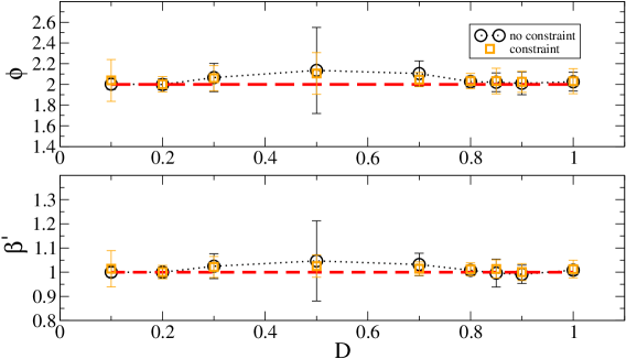
Figure 4: Behavior of the exponents $\phi$ and $\beta^{\prime}$ as a function of the diffusion rate. The circles represents the non-constrained results and the squares denote the constrained results. The dotted line is only a guide for the eyes, while the dashed lines correspond to the values $\phi=2$ and $\beta^{\prime}=1$ of the case without diffusion.

Using the method of characteristics, the equation 25 defining the approximants may be integrated. A time-like variable $\tau$ is introduced, and the partial differential equation will be equivalent to a set of two ordinary differential equations:

$$\frac{dx}{d\tau} = Q_{M}(x(\tau),y(\tau)),$$

$$\frac{dy}{d\tau} = R_{N}(x(\tau),y(\tau)).$$ (30)

The characteristics are the trajectories $(x(\tau),y(\tau))$ obtained solving these equations, and the estimate of the approximant on each characteristic may be found through integration, once we know the value on a particular point. It is possible to show that any critical line which is incident on the multicritical point will itself be a characteristic curve, and we will use this result to estimate the DP critical line in the model. The critical lines obtained by the method of characteristics are shown in the figure 5, calculated for $D=0,0.1,0.2,0.3,0.5,0.7$, and $D=0.8$.

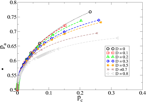
Figure 5: Critical lines obtained by the method of characteristics for different values of the diffusion rate $D$. This approach allows us to estimate the curves close to the multicritical point of DP-CDP crossover.

Once again, the approach fails to estimate the behavior for the limit of infinite diffusion rate. In fact, only values to up to $D=0.8$ could be studied with reasonable precision. On the other hand, in [10], it is shown that a good estimate of the critical line is obtained by the scaling function $x=z_{0}(1-y)^{\phi}$. A similar procedure may be applied to the model with diffusion, adopting the Ansatz $x=z_{0}(D)(1-y)^{\phi(D)}$, where $\phi(D)=2,\forall D$ and $z_{0}(D)$ is a parameter chosen to reproduce the result in a region were we have good estimates. In the figure 6 we show estimates to the critical lines from the method of characteristics and extended scaling curves for the diffusion rates $D=0.2,0.5$ and $D=0.8$. In the same figure, the extended scaling curves are depicted up to the limit of infinite diffusion rate. In that case, the curve has a maximum, unlike of the behavior of the other critical lines. Therefore, if the hypothesis that all the critical curves can be approximated by a scaling function such as $x=z_{0}(D)(1-y)^{\phi(D)}$ is true, then in the limit of infinite diffusion rate only the limiting cases $p_{b}=0$ (that equals to the CP) and $p_{c}=0$ (voter model) have the same behavior that is predicted by the mean-field for this regime.

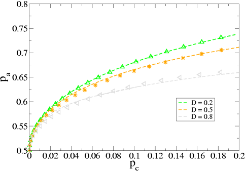
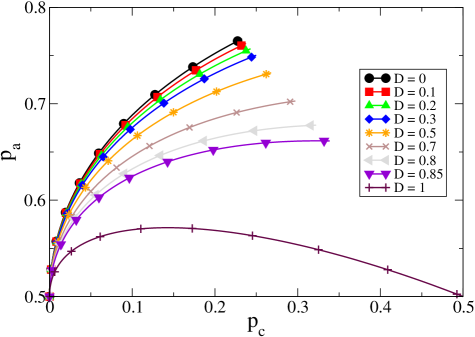
Figure 6: Top: Estimates of critical lines obtained by the method of characteristics (dashed lines) and using the extended scaling form (symbols) are compared. Bottom: Critical lines calculated using the extended scaling form $x(D)=z_{0}(D)(1-y)^{2}$ for different values of diffusion, including the infinite diffusion rate limit.

To test if the hypothesis that the critical curves can be approximated by the function $x(D)=z_{0}(D)(1-y)^{\phi(D)}$ for all value of the diffusion rate is reasonable, we calculate the behavior of $D_{eff}$ as a function of $\alpha$, in the same way as was done to obtain the curves shown in the figure 1. Remembering that $\alpha=(1-p_{a})/p_{a}$ and $D_{eff}=\alpha\tilde{D}/(1+\alpha\tilde{D})$ we fix the value of the parameter $p_{b}$ and using the values of $z_{0}(D)$ our results estimate the location the multicritical point $(\alpha_{c},D_{eff}=1)$. If mean-field behavior would be correct for all values of $p_{b}$ in the infinite rate of diffusion limit, then $\alpha_{c}$ should always be equal to one. However, as may be seen in figure 7, this value changes. We also notice that in the figure 7 an agreement between the points obtained of the critical curves estimated by the approach of the characteristics and the curves approached, giving support to the possibility of that $\alpha_{c}$ varies with $p_{b}$ and, consequently with the parameter $p_{c}$, as shown in the figure 6.

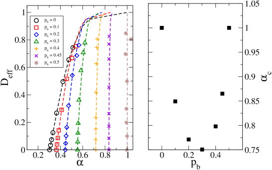
Figure 7: Phase diagrams using $\alpha$ and $D_{eff}$ as variables. For each value of parameter $p_{b}$ we have a different value for $\alpha_{c}$, that is the point where the curve achieves the infinite diffusion limit. Again the symbols are results from the method of characteristics and dashed lines are extended scaling functions.

The curves for $D_{eff}$ as a function of $\alpha$ provide another evidence of the peculiar behavior of the critical lines in the limit of infinite diffusion rate. For the CP with diffusion, at the DP-mean field change of universality class, the estimated crossover exponent is $\tilde{\phi}=4$, as found in [16]. In the figure 8 we show as this value of the exponent $\tilde{\phi}$ is obtained using the same values for $\alpha_{c}$ found in the right panel of the figure 7.

Figure 8: Log-log plots for critical curves with different values of $p_{b}$, showing that the choices of $\alpha_{c}$ from the results exhibited in figure 7 result in a crossover exponent $\tilde{\phi}=4$, as expected for the CP.

In summary, the results obtained by the PDA’s calculated for distinct values of $D$ and presented in the figure 4 are consistent with what is known in the literature [16] of the behavior expected for the crossover between the DP universality and the mean-field behavior. The results presented here seem to support the conjecture that in the limit of infinite diffusion the critical lines of the model are coincident with the simple mean field result only in the extrema, which correspond to the usual CP and the voter model.

6 Conclusion

In the generalized model without diffusion, studied using series expansions in [10], it was found that the DP-CDP crossover exponent was very close to the two-site mean-field approximation result $\phi=2$. Here we found that when diffusion is introduced in the model, the same approximation leads to $\phi=1$ for any nonzero finite diffusion rate and $\phi=0$ in the limit of infinite diffusion rate. As usual, this latter result is coincident with the one which is found applying a simple one-site mean-field approximation to the model. However, the series analyses for the model presented here support the conclusion that the introduction of diffusion does not change the crossover exponent. If this conclusion remains true in the limit of infinite diffusion, as some results above suggest, the critical line joining the points corresponding to the CP model and the voter model could not be the curve $p_{a}=1/2$ predicted by the one-site mean field approximation, since it should be a quadratic curve in the neighborhood of the multicritical point at $p_{c}=0$.

It is well known that the Padé approximants will provide poor estimates of the critical parameters in the neighborhood of a multicritical point. Actually, this was one of the motivation for the development of PDA’s, which are suited to estimate multicritical behavior [19]. As expected, Padé approximants show an increasing dispersion of the estimates as the DP-CDP multicritical point is approached, whereas PDA’s lead to good estimates in this region [10]. As diffusion is introduced in the model, we found out that PDA’s apparently are reliable for low diffusion rates, but as the rates are increased again the dispersion of estimates provided by different approximants grows and for infinite diffusion rate and no longer obtain reliable estimates from the approximants. One may suppose that, similar to the poor performance of Padé approximants close to multicritical points, the PDA’s also fail as the multicritical point of higher order is approached for infinite diffusion rate. A generalization of the PDA’s to handle a three variable series may be helpful to study this limit, and we are presently working in this direction.

Finally, in our opinion the conclusion that the crossover exponent does not change, even in the limit of infinite diffusion rate, which our results seem to support, should be viewed with some caution. We stress that in order to obtain a definite series expansion for the model, as was also necessary in earlier studies of series expansions for similar models with diffusion, we were forced to include the diffusive term into the part of the evolution operator which is treated as a perturbation, and therefore it might be possible that conclusions for high diffusion rates are misleading. Nevertheless, for low diffusion rates we may have more confidence in the results from the analysis of the series expansion, and there are clear evidences that, unlike what happens in the two-site mean field approximation, the value $\phi\approx 2$ found in the absence of diffusion, is still valid when diffusive processes are allowed.

WGD acknowledges the financial support from Fundação de Amparo à Pesquisa do Estado de São Paulo (FAPESP) under Grant No. 05/04459-1. JFS is grateful for the support provided by project PRONEX-CNPq-FAPERJ/171.168-2003.

References

References

- [1] J. Marro and R. Dickman, Nonequilibrium Phase Transitions in Lattice Models (Cambridge University Press, Cambridge, 1999)
- [2] T.E. Harris, Ann. Probab. 2, 969 (1974).
- [3] F. Schlögl, Z. Phys. 253, 147 (1972).
- [4] P. Grassberger and A. De La Torre, Ann.Phys. 122, 373 (1979).
- [5] R. M. Ziff, E. Gulari, and Y. Barshad, Phys. Rev. Lett. 56, 2553 (1986).
- [6] H. Takayasu, A. Tretyakov, and A. Yu, Phys. Rev. Lett. 68, 3060 (1992).
- [7] H. K. Janssen, Z. Phys. B, 42, 151 (1981); P. Grassberger, Z. Phys. B, 47, 365 (1982).
- [8] H. Hinrichsen, Adv. Phys.,49, 815 (2000).
- [9] W. G. Dantas, A. Ticona, and J. F. Stilck, Braz. J. of Phys. 35, 536 (2005).
- [10] W.G. Dantas and J.F. Stilck, J. Phys. A, 38, 5841 (2005).
- [11] M. Bramsom and D. Griffeath, Ann. of Prob. 9, 173 (1981).
- [12] T. M. Liggett, preprint (1994).
- [13] A. Yu. Tretyakov, N. Inui, M. Katori, and H. Tsukahara, cond-mat/9509061 (1995).
- [14] E. Domany and W. Kinzel, Phys. Rev. Lett. 53, 311 (1984).
- [15] R. Dickman and I. Jensen, J. Phys. A,26, 151 (1993).
- [16] C.E. Fiore and M.J. de Oliveira, Phys. Rev. E, 70, 046131 (2004).
- [17] I. Jensen and R. Dickman, J. Stat. Phys. 71, 89 (1993).
- [18] I. Jensen,J. Phys. A 52, 5233 (1999).
- [19] M. E. Fisher and R. M. Kerr, Phys. Rev. Lett. 32, 667 (1977).
- [20] D. F. Styer, Comp. Phys. Comm. 61, 374 (1990).