Ground-state properties of the attractive one-dimensional Bose-Hubbard model

Abstract

We study the ground state of the attractive one-dimensional Bose-Hubbard model, and in particular the nature of the crossover between the weak interaction and strong interaction regimes for finite system sizes. Indicator properties like the gap between the ground and first excited energy levels, and the incremental ground-state wavefunction overlaps are used to locate different regimes. Using mean-field theory we predict that there are two distinct crossovers connected to spontaneous symmetry breaking of the ground state. The first crossover arises in an analysis valid for large $L$ with finite $N$, where $L$ is the number of lattice sites and $N$ is the total particle number. An alternative approach valid for large $N$ with finite $L$ yields a second crossover. For small system sizes we numerically investigate the model and observe that there are signatures of both crossovers. We compare with exact results from Bethe ansatz methods in several limiting cases to explore the validity for these numerical and mean-field schemes. The results indicate that for finite attractive systems there are generically three ground-state phases of the model.

I Introduction

Systems of attractive bosons are one of the most intriguing current topics in physics. For instance they might lead the way for fabricating mesoscopic Schrödinger cat states Leggett ; Zoller , and in the experimental context, they have been used to produce the Bosenova phenomena bosenova . The substantial amount of research undertaken recently Hulet ; Salomon ; attractive-through-Feshbach ; Kanamoto ; attractive-BH-numerics ; Buonsante ; Pan ; attractive-integrable-LL-model poses new questions surrounding systems of attractive bosons. An almost ideal realisation of a lattice Bose gas - the Bose-Hubbard model - has been found in bosons trapped inside optical lattices BH-optical-lattice-realisations . The use of techniques like Feshbach resonances allows tuning of the scattering length, i.e. changing the interaction strengh, even crossing from repulsive to attractive attractive-through-Feshbach ; Salomon . The theoretical boson model predicts a dramatic change in the ground state of a large but finite system when the attractive interaction strength is varied from weak to strong attractive, see figure 1 and figure 2 for visualisation. Currently technical difficulties make experiments on attractive system considerably harder compared to repulsive system Hulet ; Salomon . Once handling and stability of attractive bosons in optical lattices allows experiments at controlled and varying interaction strengths this general transitional feature could be experimental verifiable. Potential candidates for measurements might include correlation functions, momentum distribution after release from the trap and the low-lying energy spectrum. Historically, the theoretical study of attractive bosonic systems has received little attention due to difficulties Mattis-red-book like non-saturation or high site occupancy. A number of numerical and approximative studies for a variety of attractive bosonic systems Kanamoto ; attractive-BH-numerics ; Buonsante ; Pan have found a transitional regime between the strong and the weak interacting regions. This crossover can be seen in properties like the energy spectrum Kanamoto , correlation functions Buonsante or entanglement Pan . All these properties have the common feature that the crossover becomes sharper and more pronounced for larger system sizes, a region where numerical and approximative techniques enter a region of uncertainty. A transition is also seen in studies of mean-field techniques of the non-linear Schrödinger equation in the context of the Bogolyobov approximation or in solitonic solutions of the Gross-Pitaevskii equation attractive-mean-field-1 ; attractive-mean-field-2 . Despite an early Bethe Ansatz solution LL for the continuum Bose gas with contact interactions, the exact treatment of attractive quantum systems lags behind the study of similar repulsive systems Big-Hubbard-book ; Mattis-red-book ; Korepins-book .

In this work we consider the one-dimensional periodic Bose-Hubbard model in the attractive regime, as a simple boson model with short-range interactions and local hopping term. This model is in general not integrable Haldane-Choy , but it possesses several integrable limits and displays rich transitional behavior in the ground state.

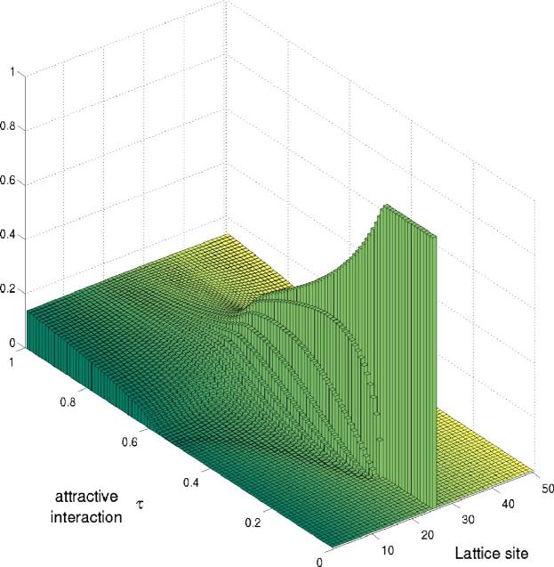
Figure 1: Generic ground-state behaviour for attractive bosons: momentum distribution of trapped bosons, within a mean-field approach for $L=50$. See also figure 2 for the real space “density“ and section III.1 for technical details. In the weak interaction region (right front in these figures: $\tau\to 0$) the system is in an ideal BEC state, all bosons are condensed into the lowest momentum and the semi-classical density is flat. For strongly interacting bosons (left rear in these figures: $\tau\to 1$) the momentum distribution is flat. while the translational symmetry in real space is broken, all bosons are on the same side. In between there is a rich cross over regime which we study in this paper.

A quantum phase transition (QPT) is usually defined as a phase transition at $T=0$ (i.e. in the ground state) under the variation of external parameters, here the attractive interaction strength. Phase transitions involve taking the thermodynamic limit, e.g. having infinitely many particles $N$ and lattice sites $L$. Attractive boson systems are conceptually different from repulsive bosons and attractive/repulsive fermions, in that such a limit cannot easily be defined as discussed later on. Nevertheless, for large but finite $N$ and $L$ the attractive boson system does display an increasingly sharp distinction beween ground-state regions, similar to finite size realisations of system. We will within this paper denote this generalisation by pre-transition and discuss its relevance as a tool for the analysis of attractive bosons.

To characterise the ground-state phases of the model, we study two key indicator properties. The first is simply the energy gap between the ground and first-excited states. For finite systems the gap never vanishes, and there is never an occurrence of ground-state broken-symmetry in the quantum model as a result. However we do observe through numerical analysis that the order of magnitude of the gap can be significantly different across different coupling regimes, which leads to a sense of relative quasi-degeneracy Kanamoto .

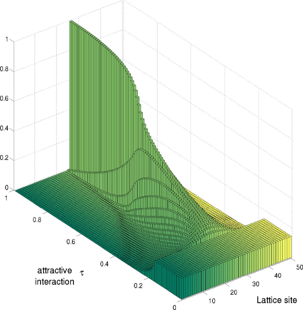
Figure 2: Real space density for attractive bosons in a trap with $L=50$ sites in a semi-classical theory. This picture is the corresponding density to figure 1, see caption for different physical regimes. Technical details text are in section III.1.

The second key property we study is the incremental ground-state wave function overlap, or the fidelity to use the language of quantum information theory. Recently there have a been a number of papers that have used this concept to study quantum phase transitions in the thermodynamic limit Zanardi ; johnpaul . The essence of this approach lies in the fact that if two states lie in different quantum phases then they are reliably distinguishable, for example through the use of an order parameter. If states are reliably distinguishable then they must be orthogonal nielsen and consequently the wave function overlap vanishes.

For finite systems we propose to modify this approach by identifying pre-transitions at couplings for which the incremental wavefunction overlap is (locally) minimal, see figure 4. For systems which exhibit a quantum phase transition in the thermodynamic limit it is then necessary that the value of the minimum goes to zero in the thermodynamic limit. In this manner we can say that the occurrence of a minimum in the incremental ground-state wavefunction overlap in a finite system is a precursor for the quantum phase transition in the thermodynamic limit. Note that the incremental overlap graphs are shown on a unitless axis as the physical interest here lies in the existence and location of minima, not the quantitative shape Semi-classical-method .

The results we find from the study of incremental ground-state wavefunction overlaps give overwhelmimg support to the mean-field results, viz. the general existence of two transitional couplings. Within the context of mean-field theory the system exhibits a broken symmetry phase. Our mean-field results point towards the existence of two transition couplings, with the critical couplings becoming degenerate at zero coupling in the limit of large particle number $N$ and a large number of lattice sites $L$. However by judiciously choosing the scaling of the parameters our findings also show that the limits $N\rightarrow\infty$ and $L\rightarrow\infty$ do not commute. For example the bosonic statistics that underly the system mean that it is possible to take $N$ to infinity while keeping $L$ finite. Moreover, we can also take $N$ and $L$ to infinity such that the “density” $N^{\mathcal{D}}/L\rightarrow$ constant for any ${\mathcal{D}}>0$. This prospect leads to the conclusion that the thermodyamic limit of the model appears to not be well-defined. This is a significant distinguishing feature compared to fermionic lattice systems such as the Hubbard model Big-Hubbard-book where the thermodynamic limit is well-defined. In section II we introduce the one-dimensional Bose-Hubbard model, list key properties used for this study and present some numerical results for small systems. Next a first analysis of the pre-transition points is given via different mean-field approaches in section III, especially the limiting case $L=2$ and $L\to\infty$ are discussed. Section IV discusses the limiting solvable cases for $L=2$ (Bose-Hubbard dimer), $N=2$ (Haldane-Choy), and $L\to\infty$ (Lieb-Liniger) via the Bethe Ansatz solution. The results of the mean-field theory and the small size exact diagonalisation are compared with these exact solutions and the limiting quasi root distribution is discussed. The discussion in section V finally puts all three approaches together and concludes that in limiting cases, e.g. very small or very large $L$, only two regions might be visible. Nevertheless, our main finding is that three ground-state phases exist in the attractive regime of model for the generic case of finite but large number of particles $N$ and lattice sizes $L$ - presumably the experimentally relevant case.

II Definition of the Model

We consider a one-dimensional Bose-Hubbard model, consisting of bosons with creation (annihilation operators) $a_{j}$ ($a^{\dagger}_{j}$) that create (annhiliate) a boson at lattice site $j$, with $j$ running over all $L$ lattice sites. The usual bosonic commutation relations such as $[a_{j},a^{\dagger}_{k}]=\delta_{jk}I$ apply. For a discussion of the physical origin and limitations of this model see exp ; BH-optical-lattice-realisations . Particles on the same site interact with interaction strength $\gamma$. The kinetic term is given by nearest-neigbour hopping with coupling strength $t$, and periodic boundary conditions $a_{L+1}\equiv a_{1}$ are imposed. In the real space presentation the Hamiltonian is given by

$$H_{\textrm{\tiny BH}}=-t\sum_{j=1}^{L}\left[a^{\dagger}_{j}a_{j+1}+a^{\dagger}_{j+1}a_{j}\right]-\gamma\sum_{j=1}^{L}a^{\dagger}_{j}a^{\dagger}_{j}a_{j}a_{j}$$ (1)

The Hamiltonian commutes with the total particle number $N=\sum_{j=1}^{L}n_{j}$ with $n_{j}=a_{j}^{\dagger}a_{j}$. The physical Hilbert space is spanned by Fock states of on-site occupation numbers $|n_{1},n_{2},...,n_{L}\rangle$ with $a^{\dagger}_{j}|n_{1},...n_{j},...n_{L}\rangle=\sqrt{n_{j}+1}|n_{1}...n_{j}+1,...n_{L}\rangle$. Its dimension ${d}=(N+L-1)!/((L-1)!N!)$ grows very rapidly with particle number and lattice size. For example, the moderate values $N=10$ and $L=20$ give the dimension of the Hilbert space as ${d}=20,030,010$, strongly limiting exact diagonalisation of systems except for the dimer and trimer system. Use of truncation schemes for the dimension and quantum Monte Carlo methods are limited by apriori unknown behavior in the transitional regions of interest.

As the Hamiltonian (1) conserves the momentum Buonsante , the matrix representation in a free momentum basis is block diagonal, and low-lying, quasi-degenerate states are characterised by differing momenta. Defining creation and annihilation operators in momentum space via the Fourier transforms $b_{k}={{L}^{-1/2}}\sum_{j=1}^{L}\exp{(\mathrm{2i}kj{\pi}/{L})}a_{j}$, $k=1...L$, it can be shown these operators satisfy canonical bosonic commutation relations $[b_{j},b^{\dagger}_{k}]=\delta_{jk}I$. The Hamiltonian (1), acting on a dual lattice of equally $L$ sites (modes) may be equivalently expressed as

$$H_{\textrm{\tiny BH}}= \ -2t\sum_{k=1}^{L}\cos\!\left(\frac{2\pi k}{L}\right)\ b^{\dagger}_{k}b_{k}$$ (2)

$$\qquad-\frac{\gamma}{L}\sum_{k,l,m,n=1}^{L}\!\!\!\!b^{\dagger}_{k}b^{\dagger}_{l}b_{m}b_{n}\delta_{k+l=m+n~{}(\textrm{mod}L)}$$

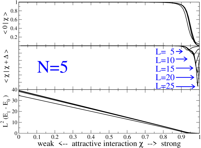
Figure 3: Results of exact numerical diagonalisation of the Bose-Hubbard Hamiltonian (1) with $N=5$ bosons and $\epsilon_{\chi}=1$ for various numbers of lattice sites $L$ (order indicated by arrows holds for all panels). The properties shown are indicators of qualitative changes in the ground state (cf. Zanardi ; johnpaul ; Kanamoto ): (top to bottom) the ground-state overlap with the non-interacting ground-state $|\chi\!=\!0\rangle$, the incremental ground-state overlap $\langle\chi|\chi+\Delta\rangle$ (for $\Delta=10^{-2}$), and the first excited energy relative to the ground-state energy. For explanations of the unitless axis in the middle graph see text. In this particular parametrisation the transitional behaviour at $\chi_{c1}\approx 0.9$, predicted by the non-linear Schrödinger equation approximation dicussed in Section III.4, is visible.

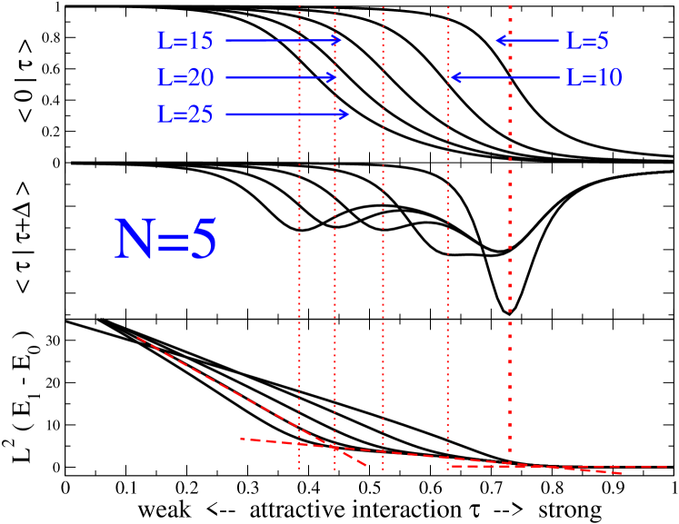
Figure 4: The same data as in figure 3, parametrised in terms of $\tau$. The dotted lines are guide to the eye, to mark three different regimes, the order of parameter $L$ indicated by arrows holds for all three panels. In this parametrisation the $L$-dependence of the pre-transition coupling $\tau_{c1}$ is apparent, as indicated by the thin dotted vertical lines. The pre-transition coupling $\tau_{c2}\approx 0.73$, as indicated by the single thick dotted vertical line, is independent of $L$ (cf. Buonsante ). At this coupling we see a minimum of the incremental ground-state overlaps and the onset of quasi-degeneracy of the ground and first energy levels. The numerical value is not in close agreement with the predicted value $\tau_{c2}=2/3$ of III.5. This discrepancy may be explained by the fact that the particle number here is $N=5$, while the analysis in section III.5 assumes large particle number.

For the remainder of this paper we only consider $t>0$ and $\gamma>0$ corresponding to attractive interactions. The model then incorporates the competition between the delocalising and localising effects of the kinetic and the interaction terms respectively. In the limit $\gamma\!\to\!0$ the ground state approaches that of non-interacting bosons, and is non-degenerate. At the other limit $t\!\to\!0$ the ground state becomes $L$-fold degenerate where the ground states consists of $N$ localised bosons on a single lattice site, viz. states of the form $|0,...0,n_{j}=N,0,...0\rangle$. However for non-zero $t$ the degeneracy is broken and the unique ground state is a superposition of these localised states, giving rise to a Schrödinger cat state. The lowest $L$ energy states in this strong interaction limit form a narrow energy band. Within mean-field theory treatments, as will be shown below, this energy band degenerates at non-zero values of $t$ giving rise to spontaneously broken translational invariance of the ground state. This provides the means to identify the ground-state phase boundaries. It had been realised Kanamoto ; Buonsante that choosing interaction parameters depending on $N$ or $L$ keeps the regions of interest centered, see figure 3 and figure 4. For the study of crossovers in the ground state the over-all energy scale can be neglected, and we introduce parametrisations mapping the whole region from the weak to the strong coupling limit into the finite interval $[0,1]$. As a dimensionless coupling parameter of the model we define $\delta=\gamma/t$, to study the ground-state properties of the model as $\delta$ is varied. To help cope with the different scaling of the regions of interest as seen above, we introduce two further parametrisations in terms of dimensionless variables $\chi,\,\tau\in[0,1]$. These are defined by

$$t=\epsilon_{\chi}(1-\chi),\qquad\qquad\gamma=\frac{\epsilon_{\chi}\chi}{NL},$$ (3)

$$t=\epsilon_{\tau}(1-\tau),\qquad\qquad\gamma=\frac{\epsilon_{\tau}\tau}{N}$$ (4)

where $\epsilon_{\tau},\,\epsilon_{\chi}$ provide the energy scale. In terms of $\delta$ we have

$$\chi=\frac{NL\delta}{1+NL\delta},\qquad\qquad\tau=\frac{N\delta}{1+N\delta}.$$

The non-interacting case is given by $\tau=\chi=0$ while pure interaction and no kinetic (hopping) contribution corresponds to $\tau=\chi=1$. Other parametrisations, e.g. logarithmic dependence, are also used in the literature Lundh . See figure 3 and figure 4 displaying the same information, for a visualisation of the effect of the parametrisation. Numerical exploration for small systems finds that the dips (local minima in the incremental ground-state overlap) are quasi-stationary for scalings of $\gamma\sim\frac{1}{N}$ and of $\gamma\sim\frac{1}{NL}$, respectively.

III Mean-Field Theory

Owing to the difficulties in treating the full quantum system with numerical and exact methods, approaching the system in the spirit of mean-field theory has been very popular. In particular with regards to investigating non-linear phenomena like solitons, and describing realistic experiments on BECs, these systems have been well studied in a wide range of contexts. The continuum limit, known as the Gross-Pitaevskii equation GPE-papers , the Lieb-Linger Bose gas or simply the non-linear Schrödinger equation (NLSE), have found wide interest continuum-MFT-papers ; Kanamoto . An extensive discussion of the mathematics of solution and further references for the discrete NLSE can be found in discrete-NLS . For the purpose of this paper we are solely focused on pre-transitions in the ground state, though, and we will not consider these applications here.

As the full discrete model is not integrable we will consider the three cases of the dimer ($L=2$), trimer ($L=3$) and the continuum limit ($L\to\infty$). We will then compare these special cases with numerical solutions to the discrete mean-field equations for generic lattice size $L$. In the last part of this section we will present a semi-classical analysis, following a different approach Carruters . We will see that it recognises the second pre-transition not visible in the continuum limit, at least qualitatively, i.e. the critical interaction scales correctly with $\sim\frac{1}{N}$, compared with $\frac{1}{NL}$ in the continuum case.

III.1 Generic $L$ and $N$

Consider the Heisenberg equations of motion for the annihilation operators $a_{j}$ in (1)

$$\mathrm{i}\frac{\textrm{d}a_{j}}{\textrm{d}t}=[a_{j},H]\ ,\qquad j=1...L$$

with restrictions to stationary solutions $a_{j}(t)=\exp({-\mathrm{i}Et})a_{j}$ for some energy eigenvalue $E$. We make the usual mean-field approximation, here expressed by replacing the operators by complex numbers

$$\vspace{-.5cm}a_{i},a_{i}^{\dagger}\qquad \longrightarrow a_{i},a_{i}^{*}\qquad\qquad$$

(operators) (complex numbers)

The resulting $N+1$ coupled equations in the $N+1$ variables $a_{1}...a_{N},E$ for the finite lattice are then given by

$$E\ a_{j}= -t\,(a_{j-1}+a_{j+1})-{2\gamma}|a_{j}|^{2}a_{j}\ ,\quad j=1,...,L,$$

$$N= \sum_{j=1}^{L}|a_{j}|^{2}$$ (5)

Note that we will discuss this procedure in Section III.4 for the continuum model again. Either way, taking the mean-field approximation first and then going to the continuum, or alternatively taking the continuum limit to the quantum Lieb-Liniger gas and afterwards replace operators by complex numbers, the result is the same continuum Gross-Pitaevskii equation.

We show a numerical solution of these equations in figure 1 and figure 2. Clearly the limiting case of (de)localisation in the densities can be seen, as well as one distinct and one less sharp crossover within this mean-field theory. A clearer picture of the pre-transitions in the semi-classical analysis is given by the indicator property shown in figure 5. The two dips scale the same, namely $\sim\frac{1}{N}$ and $\sim\frac{1}{NL}$ respectively, found from exact diagonalisation.

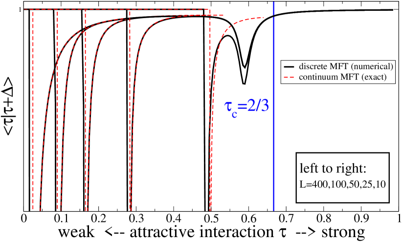
Figure 5: Ground-state wave function overlap within the mean-field model of section III.4, versus attractive interaction strengh $\tau$. The numerical solution of the discrete non linear Schrödinger equation (solid black lines) exhibits the two dips locating the two transitional points, already anticipated by figure 1 and figure 2. The continuum approximation via the exact soliton solution (section III.4) of the integrable non-linear Schrödinger equation (dashed red lines) has only one transitional point: this finite lattice effect is found in both the full quantum model and its semiclassical mean-field approximation when comparing with each respective continuum limit. Note that the exact mean-field theory result does drop off again for strong interactions, which is not shown here. Confer figure 11 for the exact solution in the case $N=2$ (Haldane-Choy). For strong interaction in this approximation the ground state does not enter a region of small changes again, thus not specifying a second transitional point, nor does it relate to the location of the lattice model transitional point, see graph for $L=10$.

As the discrete system (5) is non-integrable the general solutions are not known except for special cases. In the limit of weak interactions the ground state of the orginal system is given by the state with all particles in the zero momentum mode (an “ideal BEC”), corresponding to the constant solution $a_{i}=\sqrt{{N}/{L}},\quad i=1...N$, with energy $E=2(\tau-1-{\tau}/{L})$ (For this and the following section we set $\epsilon_{\tau}=1$). This delocalised wave function is a solution to the mean-field system for all interaction strengths, but for stronger interaction the ground state becomes a localised solution. Higher energy solutions can be constructed by considering extensions $a_{j}=\sqrt{{N}/{L}}\exp({2\pi j\phi}/L)$ or sawtooth like amplitudes. Here we are only interested in the lowest energy solution $\phi=0$. Although the particle number $N$ enters the system of equations as a parameter, this mean-field approximation shows “sharp” pre-transitions between phases regardless of the value of $N$. In the following we will first discuss the special cases of the dimer ($L=2$) and the trimer ($L=3$), before considering the case of large $L$. This non-linear system has many solutions for a given parameter $\tau$. The numerical solutions shown were obtained by starting from a known limiting case and then iterating via small changes in $\tau$. As will be seen this procedure may lead to spontaneous “hopping” to another solution once the current one ceases to exist.

III.2 Dimer $N=2$

For the dimer system the mean-field equations (5) consist of three coupled, non-linear equations for the complex variables $a_{1}$, $a_{2}$ and the energy $E$. Assuming real solutions is equivalent to finding the roots of a 4th order polynomial. Two solutions are real for the whole interaction range $0<\tau<1$, these lead to $a_{1}=\pm a_{2}$, with “$+$” being the symmetric ground-state solution (the horizontal line in figure 6). But for values of the coupling $\tau>\tau_{c2}$

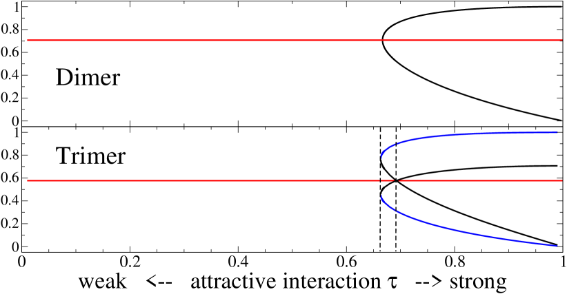
Figure 6: Occupancy of the modes for varying attractive interaction $\tau$ within the discrete non-linear Schrödinger equation approximation of section 5. Here the upper (lower) line shows either $a_{1}=a_{3}$ ($a_{2}=a_{3}$). The horizontal line denotes the constant (“ideal BEC”) solution, which exists for arbitrary $L$ and $\tau$. In the dimer there exists a pre-transition coupling $\tau_{c2}=2/3$, beyond which a second, increasingly localised solution exists. For the trimer case the pre-transition coupling in a two-height scenario is $\tau_{c2}\approx 0.663$ (left dashed line). Note that the initially dark soliton (black lines) turns into a bright soliton before it merges with the (lowest lying) bright soliton (blue lines), cf. section III.3 for details. At $\tau_{c2}$ these real solutions cease to exist, but there is no smooth connection to the constant solution as in the dimer case, indicating the lattice effect, see text for further discussion, and cf. figure 2

there opens up two new solutions with (the same) lower energy. These connect at $\tau_{c2}$ to the constant solution $a_{1}=a_{2}$. For $\tau\to 1$ the solution localises, i.e. $a_{1}\to 1$, $a_{2}\to 0$ or $a_{1}\to 0$, $a_{2}\to 1$, as shown in figure 6. The critical value $\tau_{c2}$ agrees with the semi-classical result of Sect. III.5 and an alternative mean-field treatment given in Zoller .

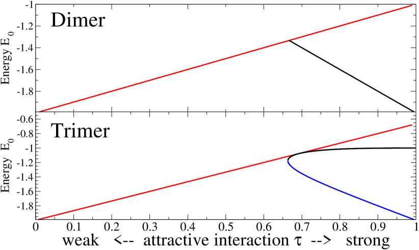
Figure 7: The energy for the lowest lying state of the two-height mean-field solution for dimer and trimer, corresponding to figure 6. Note that for $L=2$ the soliton solution connects smoothly to the constant solution. In the two-height approximation for the trimer there is already a small region around $\tau\approx 0.663$ where the true ground state is not of the two-height form. Compare this to the large middle region visible in figure 1 and figure 2, which differs from the conclusions in a recent study Buonsante .

III.3 Trimer $L=3$

The trimer system is non-integrable and it has been studied previously in the context of chaotic behaviour Milburn ; Franzosi . Here we are only interested in soliton solutions for the ground state within the mean-field description of the discrete non-linear Schrödinger equation. It is useful to introduce the notion of bright and dark solitons. A bright soliton has a localisation with positive amplitude relative to the constant solution, while the dark solition has a negative amplitude, i.e. a bright soliton looks like a hill and a dark soliton looks like a valley. For the dimer case the twice degenerate bright soliton solution is at the same time a dark soliton, as the hill and valley cannot be distinguished for $L=2$. For the trimer case $L=3$ bright and dark solitons have different energies.

Using a similar ansatz as for the dimer, i.e. $a_{2}=a_{3}$ and requiring $a_{i}$ to be real, reduces the problem to the analysis of a 4th order polynomial. A dark soliton ($|a_{2}|>|a_{1}|$) and a bright soliton ($|a_{2}|<|a_{1}|$) exist for $\tau>\tau_{a}\approx 0.663$, with the bright soliton having the lowest energy. The energies of the two solitons are the same at $\tau=\tau_{b}\approx 0.692$, which is not the point at which the bright and dark degenerate into the constant solution, i.e. $|a_{1}|\neq|a_{2}|$ at $\tau=\tau_{a}$. We remark further that at $\tau=\tau_{b}$ the dark soliton becomes a second, higher energy, bright soliton. At this point the energies for this soliton and the constant solution are the same, as shown in figure 7. This ceasing of the real solution of the form $a_{1}>a_{2}=a_{3}$ is a hint to the qualitative difference between the dimer case $L=2$, and the general case $L>2$. We expect that in a small region the ground state is neither of the constant nor of the simple two-heights soliton form, but a more complex solution connecting these both. This intermediate region does not exist for the dimer.

III.4 $L\rightarrow\infty$: Non-linear Schrödinger equation approximation

In the limit as $L\rightarrow\infty$ we can approximate the Bose-Hubbard Hamiltonian (1) by a quantum field theory, with field operator $\Psi(x)$ satisfying

$$[\Psi(x),\Psi^{\dagger}(y)]=\delta(x-y).$$

Setting $a_{j}=\sqrt{\Delta}\Psi(j\!\cdot\!\Delta)$, this consists of replacing $\Delta\sum^{L}\to\int^{\Delta L}\textrm{d}x$ under the assumption that $\Delta\ll 1$. This is to be understood as choosing $L$ very large and $N$ finite, distinct from the usual notion of the thermodynamic limit where $N,L\to\infty$ while keeping ${N}/{L}=$ constant. The implication of this approximation will be discussed later. These considerations lead to a mapping of the Bose-Hubbard Hamiltonian to the non-linear Schrödinger equation, where the latter reads

$$H_{NLS}= \int_{0}^{l}\left[\Psi^{\prime\dagger}(x)\Psi^{\prime}(x)\right]\textrm{d}x$$

$$\quad-c\int_{0}^{l}\Psi^{\dagger}(x)\Psi^{\dagger}(x)\Psi(x)\Psi(x)\textrm{d}x$$ (6)

with the periodic boundary condition $\Psi(0)=\Psi(l)$. At this point we remark that the Hamiltonian (6) is integrable Korepins-book - see section IV.3 for more details. One of the conserved operators is the total particle number

$${\mathcal{N}}=\int_{0}^{l}\Psi^{\dagger}(x)\Psi(x)\textrm{d}x$$ (7)

which is quantised and has eigenvalues which are non-negative integers. The approximation of the Bose-Hubbard Hamiltonian by the non-linear Schrödinger equation is

$$H_{BH} \approx t\Delta^{2}H_{NLS}-2t{\mathcal{N}}$$

$$N \approx {\mathcal{N}}$$

where $l=\Delta L$ and $c=\gamma/\Delta t$. Hereafter we set $l=1$ or equivalently $\Delta=L^{-1}$.

The time evolution of the field operator $\Psi$ can be determined in the usual way :

$$\mathrm{i}\frac{\partial\Psi}{\partial t} = [\Psi,H_{\textrm{\tiny NLS}}]$$ (8)

$$= -\frac{\partial^{2}\Psi}{\partial x^{2}}-2c|\Psi|^{2}\Psi$$

Our next step is to treat (8) as a classical field equation (cf. Kanamoto ). We introduce the rescaled field $\Phi=\sqrt{N^{-1}}\Psi$ and look for stationary solutions $\Phi(x,t)=\exp(-iEt)\Phi(x)$ such that

$$1= \int_{0}^{1}|\Phi|^{2}\textrm{d}x,$$ (9)

$$E{\Phi}= -\frac{\partial^{2}\Phi}{\partial x^{2}}-U|\Phi|^{2}\Phi.$$ (10)

where $U=2cN$. The ground-state symmetry breaking solution to equations (9,10) is known Kanamoto ; attractive-mean-field-1 , and reads

$$\Phi(x)\!=\!\left\{\begin{tabular}[]{ll}$1$&\ for $U<2\pi^{2}$\\ $\displaystyle\sqrt{\frac{K(m)}{E(m)}}\mathrm{dn}\!\left[2K(m)(x\textendash x_{0})|m\right]$&\ for $U>2\pi^{2}$\end{tabular}\right.$$ (13)

Above, $\mathrm{dn}(u|m)$ is a Jacobi elliptic function, $E(m)$ and $K(m)$ denote the complete elliptic integrals of the first and second kind, and $m$ is a function of $U$ Kanamoto ; attractive-mean-field-1 . Note that $x_{0}\in[0,1]$ is the coordinate of the maximum of the wave function: the spontaneous symmetry breaking in the mean-field result is visible from the degeneracy of the solutions beyond the point of “collapse” of the constant solution into a soliton at the critical coupling $U_{c}=2\pi^{2}$. In terms of the dimensionless coupling parameter $\chi$ of the Bose-Hubbard model this corresponds to

$$\delta_{c1}=\frac{\pi^{2}}{NL}$$ (14)

or equivalently

$$\tau_{c1}=\frac{\pi^{2}}{L+\pi^{2}},\qquad\ \ \chi_{c1}=\frac{\pi^{2}}{1+\pi^{2}}\approx 0.908$$ (15)

The soliton solution connects continuously, but not smoothly, to the constant solution at $\chi_{c}$ - in figure 5 this corresponds to dip in the dashed red line. A numerical solution for the finite size discrete NLSE is shown figure 1 and figure 2, here this corresponds to the sharp change at around $\tau\approx 0.2$.

III.5 $N\rightarrow\infty$: Semi-classical analysis

In this section we present an alternative type of mean-field analysis, where we start by assuming that $N$ is arbitrarily large and $L$ is fixed. This is achieved by first canonically transforming to a number-phase representation of the quantum variables.

Let $\{N_{j},\theta_{j}\}_{j=1...L}$, obey canonical relations $[\theta_{i},\,\theta_{j}]=[N_{i},\,N_{j}]=0$,  $[N_{j},\,\theta_{k}]=i\delta_{jk}$. We make a change of variables

$$b_{j}=\exp(i\theta_{j})\sqrt{N_{j}},\quad b_{j}^{\dagger}=\sqrt{N_{j}}\exp(-i\theta_{j}).$$

Using the fact $\exp(i\theta_{j})N_{j}=(N_{j}+1)\exp(i\theta_{j})$ it can be verified that the canonical commutation relations amongst the boson operators $b_{j},\,b^{\dagger}_{j}$ are preserved. For large $N_{j}$ we can approximate the Bose-Hubbard Hamiltonian (1) by

$${\mathbb{H}}=-2t\sum_{j=1}^{L}\sqrt{N_{j}N_{j+1}}\cos(\theta_{j}-\theta_{j+1})-\gamma\sum_{j=1}^{L}N_{j}^{2}$$ (16)

We now treat ${\mathbb{H}}$ as a classical Hamiltonian and look to minimise it subject to the particle number constraint

$$N=\sum_{j=1}^{L}N_{j}$$ (17)

The minimum occurs when $\theta_{j}=\theta\,\forall j$, which leads us to studying

$${\mathbb{H}}={\mathbb{H}}_{1}+{\mathbb{H}}_{2}$$

where

$${\mathbb{H}}_{1} = -2t\sum_{j=1}^{L}\sqrt{N_{j}N_{j+1}}\ ,\qquad{\mathbb{H}}_{2} = -\gamma\sum_{j=1}^{L}N_{j}^{2}$$

It can be verified that for $N_{j}=N/L\,\forall j$, ${\mathbb{H}}_{1}$ is globally minimal and ${\mathbb{H}}_{2}$ is globally maximal. Thus for any $\gamma/t$ the solution $N_{j}=N/L\,\forall j$ provides a fixed point of the system, which will be the unique global minimum when $\gamma/t$ is sufficiently small. We look to determine the coupling at which this solution ceases to be the minimum. The results of the previous section indicate that when this happens a soliton solution will emerge. We can parametrise such a soliton solution as

$$N_{j}\geq\frac{N}{L} \qquad{\rm for~{}}j\leq z,$$ (18)

$$N_{j}<\frac{N}{L} \qquad{\rm for~{}}j>z$$ (19)

where $1\leq z\leq(L-1)$. Within this classical treatment, we can approximate the ground state for the full system by the two ground-state configurations for the sublattices $j\leq z$ and $j>z$. For the full system at the pre-transition coupling $\delta_{c1}$ as predicted in III.4, we see that the systems on the sublattices are below the pre-transition coupling due to the $L$-dependence of $\delta_{c1}$. Hence the ground-state configuration across each sublattice is one where the $N_{j}$ are constant on each sublattice. This leads us to look for soliton solutions within a two-height approximation, valid close to a point of broken symmetry:

$$N_{j}=\left\{\begin{tabular}[]{ll}$\displaystyle\frac{N(1+\alpha)}{2z}$&\qquad for $j\leq z$\\[7.11317pt] $\displaystyle\frac{N(1-\alpha)}{2(L-z)}$&\qquad for $j>z$\end{tabular}\right.$$ (22)

where $-1\leq\alpha\leq 1$ is continuous, such that (17) holds.

In terms of the above parametrisation the Hamiltonian is

$${\mathbb{H}}= -tN\left(\frac{(z-1)(1+\alpha)}{z}+\frac{(L-z-1)({1-\alpha})}{L-z}\right.$$

$$\qquad\qquad\qquad+\left.2\sqrt{\frac{1-\alpha^{2}}{z(L-z)}}\right)$$ (23)

$$\qquad-\frac{\gamma N^{2}}{4}\left(\frac{(1+\alpha)^{2}}{z}+\frac{(1-\alpha)^{2}}{L-z}\right)$$

The next step is to minimise this expression for ${\mathbb{H}}$ with respect to the variables $z$ and $\alpha$, this involves mostly standard calculus techniques. We find that the smallest coupling for which symmetry-breaking of the ground state occurs is

$$\delta_{c2}=\frac{2}{N},\qquad\chi_{c2}=\frac{2L}{1+2L},\qquad\tau_{c2}=\frac{2}{3}.$$ (24)

In deriving the value $\delta_{c2}$, we justified the use of the two-height soliton approximation on the basis that $\delta_{c1}$ is a decreasing function of $L$. The fact that $\delta_{c2}$ was ultimately found to be independent of $L$ does not invalidate the two-height approximation within the context of the above analysis. The numerical results of figure 4 illustrate that in a generic finite system the gap between the ground state and first excited-state energy levels is smaller at $\delta_{c2}$ (or equivalently $\tau_{c2}$) than at $\delta_{c1}$ (or equivalently $\tau_{c1}$). Thus the notion of quasi-degeneracy of the energy levels is more appropriate at $\delta_{c2}$ than at $\delta_{c1}$.

Let us consider what happens when we now take the thermodynamic limit $N,\,L\rightarrow\infty$:

$$\delta_{c1}=0, \qquad\chi_{c1}=\frac{\pi^{2}}{1+\pi^{2}}, \tau_{c1}=0,$$ (25)

$$\delta_{c2}=0, \qquad\chi_{c2}=1, \tau_{c2}=\frac{2}{3}.$$ (26)

The fact that the two sets of values (25) and (26) do not agree is an indication that the limits $N\rightarrow\infty$ and $L\rightarrow\infty$ do not commute, meaning that the usual concept of the thermodynamic limit is not well-defined for this model. Equations (25) and (26) again show that two of the regions of interest will vanish when using the standard $\delta$ variables. When using the parametrisation in the variables $\chi$ and $\tau$ only one region disappears and one pre-transition point stays finite, i.e. away from 0 (no interaction limit) and 1 (no hopping limit).

Another curious point to observe is that while both $\chi_{c2}$ and $\tau_{c1}$ are $L$-dependent, they are in fact independent of $N$. This gives faith that the general qualitative ground-state features of the finite system will be tractable from analyses of systems with relatively small particle numbers.

IV Limiting Integrable Models

While repulsive boson systems, as well as repulsive and attractive fermion systems are well studied in the context of solvable systems the attractive boson gas received comparatively little attention attractive-integrable-LL-model . Still the seminal Bethe Ansatz solution for one-dimensional contact interaction bosons LL in the continuum describes the repulsive as well as the attractive regime, in which the solutions to the Bethe Ansatz equations become of different character  McGuire-attractive-scattering . Initially it was believed that also the Bose-Hubbard model has a Bethe Ansatz solution Haldane-Choy , but it soon turned out that this model is non-integrable. Nevertheless there are several integrable limits and extensions, see figure 8. Out of these we will examine the three limits shown inside the general Bose-Hubbard box for the case of attractive interactions.

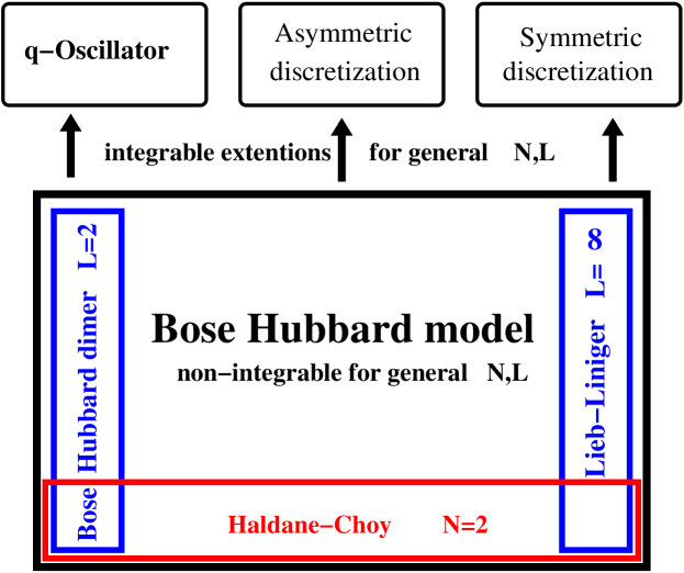
Figure 8: Integrable relatives of the Bose-Hubbard model: the 6 small boxes have Bethe Ansatz solutions, while the general Bose-Hubbard models is non-integrable.

Integrable lattice distortions of bosons on a one-dimensional lattice, for instance the three boxes on top of figure 8, have been studied mainly for the repulsive case q-oscillator ; Korepins-book ; symmetric-discretisation ; BH-quantum-chaos ; Kundu . The attractive parameter region is technically harder than the repulsive case: for instance the attractive Bethe Ansatz roots in the Lieb-Liniger model lack several of the properties which allowed analysis for repulsive interaction: e.g. string solutions which keep their string form and saturation of the root distribution in the thermodynamical limit. The problem of collapse of the system already at infinitely weak attractive interaction when taking the thermodynamic limit is less problematic Mattis-red-book and has been addressed by the $N$-dependent reparametrisation Kanamoto ; Buonsante . In the next secion IV.1 we will briefly discuss the Bethe ansatz solution of the $L=2$ dimer case and point out that it has only one crossover. Then we move on to discuss the finite lattice size case $L>2$ via the two-particle solution of the Haldane-Choy ansatz: here we see now two pre-transitions, i.e. dips in the indicator property ground-state overlap, which have the correct scaling behaviour found numerically and via semi-classical analysis earlier in this paper.

We will establish via the $N=2$ Haldane-Choy solution and the results from section III for the relation between the (discrete) NLSE and the (continuum) GPE that the integrable Lieb-Liniger continuum gas is a good proxy for the discrete lattice model for the study of the $NL$-dependent pre-transition. This motivates our discussion of the Bethe ansatz root distribution for the attractive ground state of the Lieb-Liniger model and relates these results to the Bose-Hubbard model in the last section.

IV.1 Bose-Hubbard dimer

For the dimer case, $L=2$, the Hamiltonian (1) reduces to

$$H=\textendash 2t\!\left(a_{1}^{\dagger}a_{2}+a_{2}^{\dagger}a_{1}\right)-\gamma\left(a_{1}^{\dagger}a_{1}^{\dagger}a_{1}a_{1}+a_{2}^{\dagger}a_{2}^{\dagger}a_{2}a_{2}\right).$$

This Hamiltonian can be expressed enolskii1 in terms the $su(2)$ algebra with generators $\{S^{z},\,S^{\pm}\}$ and relations

$$[S^{z},S^{\pm}]=\pm S^{\pm},\qquad[S^{+},S^{-}]=2S^{z}.$$

Using the Jordan-Schwinger representation

$$S^{+}=a^{\dagger}_{1}a_{2},\quad S^{-}=a^{\dagger}_{2}a_{1},\quad S^{z}=\frac{1}{2}(a^{\dagger}_{1}a_{1}-a^{\dagger}_{2}a_{2})$$

this leads to

$$H=-2t\left(S^{+}+S^{-}\right)-{\gamma}\left(2(S^{z})^{2}+\frac{1}{2}N^{2}-N\right).$$

The same $(N+1)$-dimensional representation of $su(2)$ is given by the mapping to differential operators

$$S^{z}=u\frac{{\rm d}}{{\rm d}u}-\frac{N}{2},\quad S^{+}=Nu-u^{2}\frac{{\rm d}}{{\rm d}u},\quad S^{-}=\frac{{\rm d}}{{\rm d}u}$$

acting on the space of polynomials with basis $\{1,u,u^{2},...,u^{N}\}$. We can then equivalently represent the dimer Hamiltonian $H$ as the second-order differential operator

$$H = -2t\left(Nu+(1-u^{2})\frac{{\rm d}}{{\rm d}u}\right)$$ (27)

$$\quad-\gamma(2u^{2}\frac{{\rm d}^{2}}{{\rm d}u^{2}}+2(1-N)u\frac{{\rm d}}{{\rm d}u}+N^{2}-N)$$

$$= -2\gamma u^{2}\frac{{\rm d}^{2}}{{\rm d}u^{2}}+\left(2\gamma(N-1)u+2t(u^{2}-1)\right)\frac{{\rm d}}{{\rm d}u}$$

$$\quad\qquad+\left(N\gamma-N^{2}\gamma-2tNu\right).$$

Now we look for solutions of the eigenvalue equation

$$HQ=EQ$$ (28)

where $Q$ is a polynomial function of order $N$ which we express in terms of its roots $\{v_{j}\}$:

$$Q(u)=\prod_{j=1}^{N}(u-v_{j}).$$

Evaluating (28) at $u=v_{k}$ for each $k$ leads to the set of Bethe ansatz equations

$$\frac{t(1-v_{k}^{2})+\gamma(1-N)v_{k}}{\gamma v^{2}_{k}}=\sum^{N}_{j\neq k}\frac{2}{v_{j}-v_{k}},\,\,k=1...N.$$ (29)

By considering the terms of order $N$ in (28) the energy eigenvalues are found to be

$$E=\gamma N(1-N)+2t\sum_{j=1}^{N}v_{j}.$$ (30)

We can transform the differential operator (27) into a Schrödinger operator dhl . Setting

$$\Psi =\exp\left(-\frac{t}{\gamma}\cosh(\sqrt{2\gamma}x)-N\sqrt{\frac{\gamma}{2}}x\right)$$

$$\qquad\quad\times\prod_{j=1}^{N}(\exp(\sqrt{2\gamma}x)-v_{j}),$$

$$\widetilde{H}=-\frac{{\rm d}^{2}}{{\rm d}x^{2}}+V(x),$$

where the potential $V(x)$ is

$$V(x)=\left(\frac{2t^{2}}{\gamma}\sinh^{2}(\sqrt{2\gamma}x)-2t(N+1)\cosh(\sqrt{2\gamma}x)\right),$$

then

$$\widetilde{H}\Psi=E\Psi$$

with $E$ given by (30) whenever the $\{v_{j}\}$ are solutions of the Bethe Ansatz equations (29). It is easily checked that the potential has a single minimum when $\gamma/t=\delta<2/(N+1)$ and two minima when $\delta>2/(N+1)$. The critical value $\delta=2/(N+1)$ agrees, to leading order in $N$, with the mean-field theory result for $\delta_{c2}$ of section III.5, cf. equations (24).

From the analysis of the Bethe Ansatz solution it can be seen the limiting case of only two lattice sites has a single transitional point, visualised in figure 9.

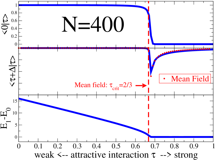
Figure 9: The Bose-Hubbard Dimer $L=2$ has a single pre-transition point. Shown are (top to bottom), ground-state wave function overlap with the non-interacting reference state, the incremental ground-state wavefunction overlap and the first excitation energy relative to the ground-state energy, each obtained by exact numerical diagonalisation. The dashed line indicates the theoretical value of $\tau_{{\rm crit}}=2/3$ which is given by mean-field theory. For the wavefunction overlaps in the middle graphic the mean-field result for the overlap are shown by the dotted line, which is barely distinguishable from the numerical result. The value obtained from the exact Bethe ansatz solution is $\tau_{BA}=2/(3(1+N^{-1}))$, giving the quantum correction to the mean-field result.

This corresponds to the case where the two minima in figure 4 coincide and the middle region is no longer visible. In figure 9 two physically very different regimes can be seen: the ground-state overlap measures the relative weight the occupation of the zero momentum mode by all particles has (relative to the non-interaction BEC state with 100% condensation at $\tau=0$). For small $\tau$ these contributions dominate, while after a small crossover region for large $\tau$ this non-interacting BEC state has a very low relative weight in the ground state. In the complementary plot, against the $N$-body Schödinger cat-state $|N,0\rangle+|0,N\rangle$ as reference state, the overlap would be almost constant, close to $1$ in the strong interacting regime on the right, while it would be $\ll 1$ and quasi-constant in the weak interacting region: the relative weight of a localisation of N particles is low. Similar for the bottom picture in figure 9: the ground-state energy for the very weakly interacting regime $\tau\approx 0$ is non-degenerate, the first excitation is separated by the energy required to transfer a single boson from the zero momentum mode to the first momentum. In the strong interacting limit for large $\tau$ the ground state is quasi degenerate : the (anti-)symmetric cat states $|N,0\rangle\pm|0,N\rangle$ have the same energy.

The mean-field calculation for the dimer, see figure 6, shows the (square root of) the relative occupancy of the two sites. For $\tau$ below the critical interaction both sites are equally occupied, the totally delocalised constant solution, with all the particle in the lowest momentum mode $b_{0}$. At $\tau_{c}=\frac{2}{3}$ the symmetry breaks and one site has higher occpuation than the others. Due to the quantum-mechanical superposition in eigenstates this can only be seen in the mean-field theory. The second momentum mode has a finite and increasing occupation beyond the critical interaction, though, and it reaches $n_{k=0}=n_{k=1}=\frac{1}{2}$ for $\tau\to 1$. This is the complete delocalisation in momentum space and corresponds to the complete localisation in real space density observed in the soliton solution.

IV.2 Haldane-Choy Bethe Ansatz for $N=2$

The Bose-Hubbard model (1) has a Bethe Ansatz solution in the spirit of the fermionic Hubbard model, but it is only solvable for a maximum site occupation of two particles Haldane-Choy . For $N=2$ the exact eigenstates are

$$\left|\mathrm{BA}\right\rangle= \sum_{i,j=1}^{L}C_{ij}|i,j\rangle$$

$$C_{nm}= \left\{\begin{tabular}[]{ll}$\mathrm{e}^{\mathrm{i}\left(kn+qm\right)}+\frac{\sin k-\sin q-\mathrm{i}\gamma}{\sin k-\sin q+\mathrm{i}\gamma}\mathrm{e}^{\mathrm{i}\left(qn+km\right)}$&$,\ \ n\leq m$\\ $C_{mn}$&$,\ \ n>m$\end{tabular}\right.$$ (33)

with the Bethe Ansatz equations

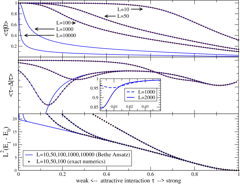
Figure 10: Similar to figure 4 for the solvable case of two bosons in a lattice of differing size $L$ (order indicated by arrows holds for all three panels) Already for the minimal particle number $N=2$ the two pre-transition points can be clearly seen, compared to the one pre-transition point for the dimer, see figure 9. The exact Bethe Ansatz solution (37) (solid lines), available for arbitrary $L$, is compared with exact numerics (dots) for small sizes. Shown are (top to bottom): the ground-state overlap with the non-interacting ground state $|\tau\!=\!0\rangle$, the incremental overlap $\langle\tau|\tau+\Delta\rangle$ for $\Delta=10^{-2}$, and the first excited energy relative to the ground state $L^{2}(E_{1}-E_{0})$.

$$\mathrm{e}^{\mathrm{i}kL}=\frac{\sin k\!-\!\sin q\!-\!\mathrm{i}\gamma}{\sin k\!-\!\sin q\!+\!\mathrm{i}\gamma}\ \,\wedge\ \,\mathrm{e}^{\mathrm{i}qL}=\frac{\sin q\!-\!\sin k\!-\!\mathrm{i}\gamma}{\sin q\!-\!\sin k\!+\!\mathrm{i}\gamma}$$ (34)

Here ​ $|i,j\rangle=a^{\dagger}_{i}a^{\dagger}_{j}|0\rangle$ is not normalised, i.e. $\langle i,j|i,j\rangle=1$ respectively $=2$ for $i\neq j$ respectively $i=j$. The energy eigenvalues for these are $E=-2(\cos k+\cos q)$, motivating the name “quasi-momenta” for the Bethe Ansatz roots $k$ and $q$. The Bethe Ansatz roots for the ground state are symmetric, $k=-q$, and imaginary for attractive interactions $\gamma>0$. For this setting we can define $k=-q=\mathrm{i}K$, with $K>0$ determined by the single Bethe Ansatz equation, here in inverse form

$$\gamma(K)=2\sinh K\ \tanh\frac{KL}{2}.$$ (35)

For use in the next section we also note that for $\gamma>\frac{4}{L}\cos\frac{\pi}{L}$ the two real roots of the BAE solution for the first excitation $E_{1}$ merge to a complex 2-string of the form $k,q=\frac{\pi}{L}\pm\mathrm{i}K$ with $K>0$, and the inverse function given by $\gamma(K)=2\cos\frac{\pi}{L}\coth\frac{KL}{2}\sinh K$. The real roots of the first excitation for $\gamma<\frac{4}{L}\cos\frac{\pi}{L}$ are given by $k=K$, $q=\frac{2\pi}{L}-K$ with $0<K<\frac{\pi}{L}$. The inverse function relating the parameter $K$ to the interaction strength is $\gamma(K)=2\cos\frac{\pi}{L}\tan\frac{KL}{2}\sin\frac{KL-\pi}{L}$. We use these expressions for the analysis of the indicator properties like $L^{2}(E_{1}-E_{0})$, in figure 10, as well as for comparison with the Lieb-Liniger continuum model in the next section.

The (not normalised) ground-state wave function can be written as, cf. (41):

$$|K\rangle= \sum_{n,m}\left[\mathrm{e}^{K(\frac{L}{2}-|n-m|)}+\mathrm{e}^{-K(\frac{L}{2}-|n-m|)}\right]|n,m\rangle$$ (36)

$$= \sum_{n,m}\left[2\cosh K(|n-m|-\frac{L}{2})\right]|n,m\rangle$$

resulting in the closed form expression for the (not normalised) overlap in the Haldane-Choy model

$$\left\langle K\!+\!\Delta|K\!-\!\Delta\right\rangle=\hskip 130.88284pt$$ (37)

$$4L\left(\coth K\coth K\,L+\coth\Delta\coth\Delta\,L\right)$$

together with the normalisation

$$\langle K|K\rangle=L\mathrm{e}^{-KL}\left(\coth K-1\right)\hskip 85.35826pt$$

$$\times\left(2L\mathrm{e}^{K(L+2)}-2L\mathrm{e}^{KL}+\mathrm{e}^{2K(L+1)}+\mathrm{e}^{2KL}-\mathrm{e}^{2K}-1\right)$$

this results in the normalised overlap expression

$$\frac{\langle K+\Delta|K-\Delta\rangle}{\sqrt{\langle K+\Delta|K+\Delta\rangle\langle K-\Delta|K-\Delta\rangle}}.$$

In the above equations $K\pm\Delta$ denote the imaginary parts of the single Bethe Ansatz root associated with the two different interaction strengths $\tau_{1}\mapsto K+\Delta$ and $\tau_{2}\mapsto K-\Delta$, i.e. solutions to (35). This expression depends on the interaction strength $\gamma$ only through the Bethe Ansatz root $K$, allowing closed form solution in parametrised form . The Bethe Ansatz solution for only two particles is not truly a many-particle solution - the $N=2$ Bose-Hubbard model can be treated exactly conventionally in center-of-mass coordinates Fluegge ; rep-BH-experiment . In that case the physical meaning of the Bethe Ansatz quasi-momenta is lost, though. The solution presented here is visualised in figure 10. We remark that within this approach the exact momentum distribution of two bosons in the one-dimensional lattice can be calculated explicitly, clarifying the connection between the (here two) Bethe Ansatz quasi-momenta and the physical momenta, which is of interest for example in the integrable boson-fermion mixture our-mixture .

IV.3 Lieb-Liniger approximation

The continuum model in (6) is the integrable Lieb-Liniger gas LL . For the repulsive regime it is arguably one of the best studied integrable models LL ; Mattis-red-book ; Takahashi-book ; Korepins-book ; weak-bosons ; LL-repulsive-studies , while the attractive regime is less popular attractive-integrable-LL-model , due to difficulties in taking the thermodynamic limit. When taking the limit $L\to\infty$ in the Bose-Hubbard model the Lieb-Liniger model can be used as an integrable approximation for the weak coupling limit. Information is lost in taking this limit, i.e. in going from the three independent parameters $N,L,\gamma$ of the Bose-Hubbard model to the two parameter continuum model. Thus we expect the range of validity to be restricted, but in turn the property of integrability is gained. There are two different ways of looking at this integrable model as a limit of the Bose-Hubbard model, we consider the analysis for finite $N$ and large $L\to\infty$ in section IV.3.1. For repulsive interactions the thermodynamic limit can very succesfully be treated (see Korepins-book for references) for constant density $n=\frac{N}{L}$ when $N,L\to\infty$. In the first case the two independent parameters are $N$ and an interaction strength. In the second case we keep the particle density/filling factor $n$ and an interaction strength as free parameters. This physical notion of density (of Bethe ansatz roots) is not extendable to the attractive case, the bosons tend to cluster up instead of saturating. We discuss this further in section IV.3.2.

IV.3.1 Analysis for finite $N$ and large $L\to\infty$

In this section we analyze the special case $N=2$ as example for finite $N$ and (very much) larger $L\gg N$. The exact Haldane-Choy solution discussed in section IV.2 is the yardstick to explore the impact of the continuum approximation in the full quantum model. The energy eigenvalues in the general Lieb-Liniger model corresponding to an approximated lattice model are given by

$$L^{2}E=\sum_{i=1}^{N}k_{i}^{2}\ +\textrm{const.}$$ (38)

with the $N$ complex parameters $k_{i}$ determined by solutions to the Bethe ansatz equations

$$\mathrm{e}^{\mathrm{i}k_{i}}= \prod_{j\neq i}^{N}\frac{k_{i}-k_{j}-\mathrm{i}\tau\frac{L}{N}}{k_{i}-k_{j}+\mathrm{i}\tau\frac{L}{N}}\ ,\qquad i=1...N$$ (39)

In particular we see that the continuum model gets mapped onto the weak coupling limit of the lattice model, as $\frac{N}{L}\to 0$ for $N=2$ and $L\to\infty$. To check how well the Lieb-Liniger model approximates the Bose-Hubbard model for large $L$ we calculate analytically the ground-state overlap for the case $N=2$ and compare with the Haldane-Choy expression (37). The root behavior for ground state and first excitation (see also appendix of LL ) is similar to the lattice case: the two ground-state roots form again a purely imaginary complex pair $k_{1,2}=\pm\mathrm{i}K$, where the inverse function is given by

$$\gamma=2\,\frac{K}{L}\tanh\frac{K}{2}.$$ (40)

The first excitation roots form a complex pair past the interaction strength $\gamma>\gamma_{c}=\frac{4}{L}$ of the form $k_{1,2}=\pi\pm\mathrm{i}K$, with inverse function $\gamma=2\,\frac{K}{L}\coth\frac{K}{2}$. For weak interaction $\gamma<\gamma_{c}$ the first excitation has two real roots at $k_{2}=2\pi\textendash k_{1}=2\pi\textendash K$, with inverse function $\gamma=\frac{2}{L}(\pi\textendash K)\tan\frac{K}{2}$.

The (not normalised) ground-state wave function for finite interaction and $N=2$ is given by, cf. (36)

$$\left|K\right>= \mathrm{e}^{+K(|x-y|-\frac{1}{2})}+\mathrm{e}^{-K(|x-y|-\frac{1}{2})}$$ (41)

$$= 2\cosh K(|x-y|-\frac{1}{2})$$

The normalised ground-state wavefunction overlap for two different interaction strengths, with corresponding imaginary part of roots $K\pm\Delta$, is given by, cf. (37)

$$\left<K+\Delta|K-\Delta\right>$$ (42)

$$= \left(\frac{\sinh(K)}{K}+\frac{\sinh(\Delta)}{\Delta}\right)$$

$$\times \sqrt{\frac{K^{2}-\Delta^{2}}{(K-\Delta+\sinh(K-\Delta))(K+\Delta+\sinh(K+\Delta))}}$$

The comparison for $N=2$ of the rescaled Lieb-Liniger gas with the Bose-Hubbard system is shown in figure 11.

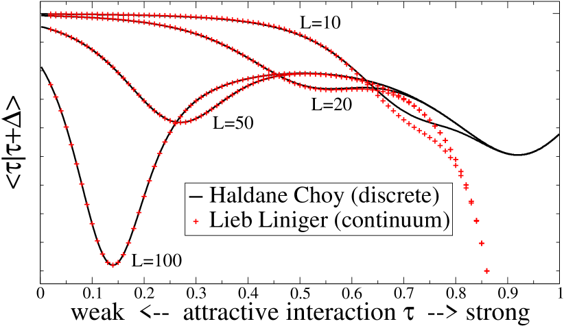
Figure 11: Ground-state wave function overlap versus attractive interaction strength $\tau$ for $N=2$ bosons. The exact solution of the full quantum model (black solid lines) on the finite lattice (Haldane-Choy) exhibits two minima, indicating two transitional points. The continuum approximation via the Lieb-Liniger model (red crosses) discussed in section IV.3.1 displays only one minimum, indicating it has only one transitional point, see text and cf. figure 5 for the large $N$ mean-field result. Note that the agreement is best in the $L$-dependent weak regime (left side) and not in the the $L$-independent strong interaction regime (right side).

From the exact diagonalisation of small systems, see figure 4 and figure 10, it is apparent that for increasing lattice size $L$ and fixed particle number $N$ a growing region extends from the strong interaction limit $\tau=1$ to smaller $\tau$. The shown physical properties in this region are independent of $L$, nevertheless the $L\to\infty$ Lieb-Liniger model is not a valid approximation for that region: from the Bethe Ansatz equations (34) and (39) it can be seen that the interaction strength gets rescaled by $\sim L^{-1}$, effectively mapping the Lieb-Liniger model onto the infinitely weak interacting Bose-Hubbard model by quasi-linearising the roots. The continuum limit does not capture the physics in the strong interaction region, in particular it does not see the second pre-transition point $\tau_{c2}$ connected to the finite lattice effect.

Our results for the semi-classical and the exact solution in the two-particle sector for the quantum model indicate that this limit is useful for the first crossover, though.

IV.3.2 Analysis of Lieb-Liniger equations for large $N$

The complicated form of the wave function within the coordinate Bethe Ansatz makes a straight forward extension of the ground-state wave function overlap calculation similar to equation (42) for the two-particle case impossible. There exist determinant formulations via the Algebraic Bethe Ansatz Korepins-book . These have been studied for the repulsive case only, though.

In the general Lieb-Liniger equations the first excited energy is relatively complicated to treat, as the root pattern is not as simple as in the $N=2$ case. It can be shown that the roots never merge into the true $N$-string for $N>2$ for total momentum one, as this would violate hermiticity . The ground-state root configuration is more accessible, as it is generally believed to be an ideal $N$-string: the roots are purely imaginary and distributed symmetrically around the origin. The limit of strong interaction or very large box size $L$ has been previously studied: the roots are then asymptotically linear in the interaction Takahashi-book and evenly spaced. In this limit the (not normalised) wave function is of the McGuire form McGuire-attractive-scattering ; Mattis-red-book

$$\Psi(x)=\exp\left({-\frac{|\gamma|}{2}\sum_{i<j}|x_{i}-x_{j}|}\right)$$ (43)

which is also relevant to (infinite length) optical waveguides Lai-waveguide .

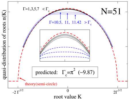
Figure 12: Quasi-distribution of the Bethe ansatz roots $n(K)$ for numerical solution of (44) with interaction $\Gamma$ below the pre-transition value $\Gamma_{c}=\pi^{2}$. The roots follow the semi-circle law (48), found analytically in the weak coupling limit $\Gamma\to 0$. The numerical results for $N=51$ are in agreement with the notion that the semi-circle law holds asymptotically for $\Gamma<\Gamma_{c}$ for sufficiently large $N$, while for $\Gamma>\Gamma_{c}$ the distribution is uniform. The dashed blue lines show the start of the finite size crossover from the semi-circle towards the box shape (49). The inset is an enlargement of the center region where the inner-lying roots approach the uniform density first.

To analyse the attractive ground state of an abstract system of equations of Lieb-Liniger type we introduce the real variables $K_{j}$ via $k_{j}\to\mathrm{i}K_{j}$. It is ad-hoc assumed that for finite interaction and finite $N$ there exists a unique real solution to

$$\mathrm{e}^{K_{i}}=\prod_{j\neq i}^{N}\frac{K_{i}-K_{j}+\frac{\Gamma}{N}}{K_{i}-K_{j}-\frac{\Gamma}{N}},\qquad i=1...N\,.$$ (44)

Here $\Gamma=cN$ is the rescaled interaction. Note the similarity of these ground state equations to systems with hard wall boundary conditions our-HW-paper ; Gaudin-book due to the externally imposed symmetry of the roots. The formulation of the problem in terms of the variables $\{K_{i}\}$ and $\Gamma$ allows the definition of a sensible distribution or quasi-density of Bethe Ansatz roots for very large but finite particle numbers $N$. Here it is useful to define a quasi-density of the roots $K_{i}$, which for example can be done via our-mixture

$$n(x)=\left\{\begin{tabular}[]{ll}$\frac{1}{N-1}\frac{1}{K_{i+1}-K_{i}}$&\qquad$x\in(K_{i},K_{i+1}]$\\ $0$,&\qquad$|x|>K_{\textrm{max}}$\end{tabular}\right.$$ (47)

In the weak coupling limit the root distribution of the real solution to (44) follows a semi-circle law derived from the relation to the Hermite polynomials Gaudin-book ; weak-bosons

$$n(K)=\frac{1}{2\pi\Gamma}\sqrt{K^{2}_{\textrm{max}}\textendash K^{2}},\quad|K|\leq K_{\textrm{max}}=2\sqrt{\Gamma}$$ (48)

In the strong interaction limit the application of the string hypothesis leads to a uniform, box shaped density. When constructing a string solution to (44) for fixed $N$ and increasing $\Gamma\to\infty$ the difference between closest roots is asymptotically $K_{i+1}-K_{i}=\frac{\Gamma}{N}$. Summing up over the symmetric root distribution it follows that $K_{\textrm{max}}=\frac{\Gamma}{2}\frac{N-1}{N}\to\frac{\Gamma}{2}$, this agrees with numerical exploration for small particle numbers $N<50$.

$$n(K)=\frac{1}{2K_{\textrm{max}}},\qquad|K|\leq K_{\textrm{max}}=\frac{1}{2}{\Gamma}$$ (49)

The above expansions hold in the limits of $\Gamma\to 0$ (weak) and $\Gamma\to\infty$ (strong), respectively, while $N$ (large) is held constant. Note that $K_{\textrm{max}}$ is in both cases independent of the particle number $N$. This would allow, at least in principle, to explore the interesting limit $N\to\infty$ for a fixed and finite interaction strength $0<\Gamma<\infty$. It is technically hard to relate the Bethe Ansatz roots in Lieb-Liniger type models to physical properties within the exact approach. Nevertheless, it is expected that the quasi-distribution (47) of the Bethe Ansatz roots in (44) for large $N$ (resp. $N\to\infty$) will show qualitatively different behaviour in the two regions $\Gamma<\Gamma_{c}$ and $\Gamma>\Gamma_{c}$, see figure 12 for numerical results for $N=51$.

For weak interaction $\Gamma\ll\Gamma_{c}$ the numerical solution $\{K_{i}\}$ is distributed approximately as a semi-circle (48), while for $\Gamma\gg\Gamma_{c}$ the quasi-density approaches a uniform box shape (49). Numerical results for small system sizes suggest an agreement with the expected value $\Gamma_{c}=\pi^{2}$ separating the two regions, where $\Gamma_{c}$ is the location of the single minima in the ground state wave function overlap in the continuum model as discussed in the earlier sections of this paper.

Numerical solutions to finite $N$ Lieb-Liniger equations are usually found by starting with an initial guess of the roots in a known region, e.g. the weak coupling limit. Then the interaction is increased in small steps $\Gamma\to\Gamma+\Delta$ where $N$ remains necessarily constant. This so called root tracking works well if the root set $\{k_{i}\}|_{\Gamma+\Delta}$ is similar to the previous step $\{k_{i}\}|_{\Gamma}$ - for a close initial guess most non-linear solver have good convergence. From the above it can be seen that this method is unsuitable for the study of large $N$ behavior - the root pattern is expected to change strongly when crossing over the pre-transition at $\Gamma_{c}=\pi^{2}$, which is in accordance with findings of Sakman et al. attractive-integrable-LL-model . In a diagram $N$ vs. $\Gamma$ the above method corresponds to moving along horizontal lines, where in the left part the root distribution is asymptotically of semi-circle shape, while on the right side it has the uniform box shape. Using that the quasi-density (47) for finite particles is in one-to-one correspondence with the root set $\{K_{i}\}$ the system (44) can be solved on vertical lines, i.e. for fixed interaction $\Gamma$ and increasing $N$. In that way the solution is stable, i.e. it does not change significantly for increasing $N$ as the pre-transition point is not crossed.

The preliminary numerical results obtained by root tracking agree with the behavior described above. Nevertheless, a rigorous analysis of (44) is necessary to determine if a quantum phase transition occurs. In particular the critical value $\Gamma_{c}=\pi^{2}$ has not been found from the Bethe Ansatz equations. This result will be relevant for the description of the first pre-transition of the initial finite size Bose-Hubbard model, when transforming the considered abstract system back to the physical problem.

V CONCLUSIONS

In this paper we have argued that there are signs of transitional behavior in the ground state of the attractive one-dimensional Bose-Hubbard model. A discussion using conventional Quantum Phase transitions - defined in the thermodynamic limit of many particles $N$ on many sites $L$ - is unsuitable as the standard limit for attractive bosons is subject to instant collapse. Instead we have used the notion of pre-transitions, characterised by a sudden change in the ground-state properties when crossing a threshold interaction strength in a system of large but finite size $N$, $L$.

Such pre-transitions are visible in indicator properties as for instance the energy gap between ground state and 1st excitation indicating onset of degeneracy, and local minima in the incremental overlap $\langle\tau+\Delta|\tau\rangle$, where $|\tau\rangle$ is the ground state for attractive interaction strength $\tau$.

We have used mean-field like approximations and integrable limits of the model to examine regions inaccessible to exact diagonalisation, and compared with exact numerics where applicable. The transitional region depends on both lattice size $L$ and number of bosons $N$ in a non-trivial way. For specific parametrisations of the coupling strength between the kinetic and the interaction contributions in the Hamiltonian one of the crossover points is quasi stationary while the other wanders. In particular we have shown that in the limit of very small and very large lattice size $L$, the complex transitional regime reduces to only two regimes with one single crossover point, in agreement with earlier studies on these models. The ground state is predicted to change strongly in a small region around critical attractive interactions. In experiments with controlled change of attractive interaction this should have clearly visible effects in properties like correlation functions and momentum distribution. If ultracold quantum gases with large but finite particle number $N$ and lattice size $L$, enter the strong attractive interaction region the validity of the physical description by the simple Bose-Hubbard model needs to be carefully investigated, though. In addition it will be interesting to see how this transitional behavior manifests in theories of more complex attractive boson systems, as we believe this is a generic feature of attractive bosonic systems rather than a speciality of this particular model. The generalisations already studied in the repulsive regime like long-range hopping, long-range interactions and extensions of lattice geometry to ladders and square lattices are an obvious starting point for further exploration. For these systems there are currently few methods available using integrable techniques.

References

- (1) A J Leggett, Rev. Mod. Phys. 73 307 (2001)
- (2) J I Cirac, M Lewenstein, K Mõlmer and P Zoller, Phys. Rev. A 57 1208 (1998)
- (3) E A Donley, N R Claussen, S L Cornish, J L Roberts, E A Cornell and C E Wieman, Nature 412 295 (2001); J L Roberts, N R Claussen, S L Cornish, E A Donley, E A Cornell and C E Wieman, Phys. Rev. Lett. 86 4211 (2001); D Voss, Science 291 2301 (2001); S Wüster, J J Hope and C M Savage, Phys. Rev. A 71 033604 (2005)
- (4) J M Gerton, D Strekalov, I Prodan and R G Hulet, Nature 408 692 (2000)
- (5) L Khaykovich, F Schreck, G Ferrari, T Bourdel, J Cubizolles, L D Carr, Y Castin and C Salomon, Science 296 1290 (2002)
- (6) S L Cornish, S T Thompson and C E. Wieman, Phys. Rev. Lett. 96 170401 (2006); S L Cornish, N R Claussen, J L Roberts, E A Cornell, and C E Wieman Phys. Rev. Lett. 85 1795 (2000)
- (7) R Kanamoto, H Saito and M Ueda, Phys. Rev. A 67, 013608 (2003); R Kanamoto, H Saito and M Ueda, Phys. Rev. A 68, 043619 (2003); R Kanamoto, H Saito and M Ueda, Phys. Rev. A 73, 033611 (2006); R Kanamoto, H Saito and M Ueda, Phys. Rev. Lett. 94, 090404 (2005)
- (8) P Buonsante, V Penna and A Vezzani, Phys. Rev. A 72 043620 (2005); P Buonsante, P Kevrekidis, V Penna and A Vezzani, J.Phys. B 39 S77 (2005)
- (9) F Pan and J P Draayer, Phys. Lett. A 339 403 (2005)
- (10) M W Jack and M Yamashita, Phys. Rev. A 71 023610 (2005)
- (11) D S Lee and D Kim, J. Korean Phys.Soc. 39 203 (2001); J G Muga and R F Snider, Phys. Rev. A 57 3317 (1998); K Sakmann, A I Streltsov, O E Alon and L S Cederbaum, Phys. Rev. A 72 033613 (2005); Y Hao, Y Zhang, J Q Liang and S Chen, Phys. Rev. A 73 063617 (2006)
- (12) I Bloch, Nature Physics 1 23 (2005); D Jaksch and P Zoller, Annals of Physics 315 52 (2005)
- (13) D C Mattis (editor), The Many-Body Problem, Chapter 5, World Scientific, Singapore (1993)
- (14) L D Carr, C W Clark and W P Reinhardt, Phys. Rev. A 62 063611 (2000)
- (15) L D Carr and Y Castin, Phys. Rev. A 66, 063602 (2002); G M Kavoulakis, Phys. Rev. A 67 011601(R) (2003), Phys. Rev. A 69 023613 (2004)
- (16) E H Lieb and W Liniger, Phys. Rev. 130, 1605 (1963)
- (17) M A Nielsen and I L Chuang, Quantum computation and quantum information (Cambridge University Press, 1999)
- (18) C Dunning, K E Hibberd and J Links, J. Stat. Mech.: Theor. Exp P11005 (2006)
- (19) V Z Enol’skii, M Salerno, N A Kostov and A C Scott, Phys. Scr. 43 229 (1991).
- (20) L P Pitaevskii and S Stringari, Bose-Einstein Condensation, Oxford University Press (2003)
- (21) P J Y Louis, E A Ostrovskaya, C M Savage and Y S Kivshar, Phys. Rev. A 67 013602 (2003)
- (22) M Duncan, A Foerster, J Links, E Mattei, N Oelkers and A P Tonel, Nucl.Phys. B in press (arXiv:quant-ph/0610244)
- (23) P Carruters, Rev. Mod. Phys. 40 411 (1968)
- (24) D E Pelinovsky, Nonlinearity 19 2695 (2006)
- (25) V E Korepin, N M Bogoliubov and A G Izergin, Quantum Inverse Scattering Method and Correlation Functions, Cambridge University Press (1993)
- (26) F H L Essler, H Frahm, F Göhmann, A Klümper and V E Korepin, The One-Dimensional Hubbard Model, Cambridge University Press (2005)
- (27) M T Batchelor, X W Guan and J B McGuire, J. Phys. A 37 L497 (2004)
- (28) M T Batchelor, X W Guan, C Dunning and J Links, J. Phys. Soc. Jpn.74 Suppl. 53-56 (2005); M T Batchelor, X W Guan, N Oelkers and C. Lee, J. Phys. A 38 7787 (2005); M Wadati, J. Phys. Soc. Jpn.71 2657 (2002); G Kato and M Wadati, Chaos, Solitons and Fractals 15 849 (2003); T Iida and M Wadati, J. Phys. Soc. Jpn.72 1874 (2003)
- (29) S Sachdev, Quantum Phase Transitions, ch. 10, Cambridge University Press (1999); M Lewenstein, A Sanpera, V Ahufinger, B Damski, A S De and U Sen, arXiv:cond-mat/0606771
- (30) L Amico and V E Korepin, Annals of Physics, 314/2 496 (2004)
- (31) A Kundu and O Ragnisco, J. Phys. A 27 6335 (1999)
- (32) E Lundh, Phys. Rev. A 70 033610 (2004)
- (33) K Nemoto, C A Holmes, G J Milburn and W J Munro, Phys. Rev. A 63 013604 (2000)
- (34) M Gaudin La fonction d’onde de Bethe, Masson (1983)
- (35) N. Oelkers, M.T. Batchelor, M. Bortz and X.W. Guan, J. Phys. A 39 1073 (2006)
- (36) M Takahashi, Thermodynamics of One-Dimensional Solvable Models, Cambridge University Press (2003)
- (37) Y Lai and H A Haus, Phys.Rev. A 40 854 (1989)
- (38) J Links, H-Q Zhou, R H McKenzie and M D Gould, J. Phys. A 36 2004 R63-R104
- (39) F D M Haldane, Phys. Lett. A 80 281 (1980) & 81 545 (1981); T C Choy and F D M Haldane, Phys. Lett. A 90 83 (1982)
- (40) J B McGuire, J. Math. Phys. 5 622 (1964)
- (41) M T Batchelor, M Bortz, X W Guan and N Oelkers, Phys. Rev. A 72 061603(R) (2005)
- (42) Z-J Ying, Y-Q Li and S-J Gu, J. Phys. A 34 3939 (2001)
- (43) P. Zanardi and N. Paunković, Phys. Rev. E 74 031123 (2006)
- (44) H.-Q. Zhou and J. P. Barjaktarevic, Fidelity and quantum phase transitions, arXiv:cond-mat/0701608
- (45) M Bortz and S Sergeev, Eur.Phys. J. B 395 (2006); M Bortz, J. Stat. Mech. P 08016
- (46) N M Bogolyubov, Translated from Teoreticheskaya i Matematicheskaya Fizika 67 451 (1986)
- (47) S Flügge, Practical quantum mechanics, Springer, Berlin -New York (1999)
- (48) K Winkler, G Thalhammer, F Lang, R Grimm, J Hecker Denschlag, A J Daley, A Kantian, H P Büchler and P Zoller, Nature 441 853 (2006)
- (49) R Franzosi and V Penna, Phys. Rev. E 67 046227 (2003)