Anomalous Binder Cumulant and Lack of Self-averageness
in Systems with Quenched Disorder

Abstract

The Binder cumulant (BC) has been widely used for locating the phase transition point accurately in systems with thermal noise. In systems with quenched disorder, the BC may show subtle finite-size effects due to large sample-to-sample fluctuations. We study the globally coupled Kuramoto model of interacting limit-cycle oscillators with random natural frequencies and find an anomalous dip in the BC near the transition. We show that the dip is related to non-self-averageness of the order parameter at the transition. Alternative definitions of the BC, which do not show any anomalous behavior regardless of the existence of non-self-averageness, are proposed.

The characterization of phase transitions relies mainly on the singularity structure of physical quantities at the transition, which can be quantified by critical exponent values. In numerical efforts, the accuracy of the estimated exponents heavily depends on the precision of locating the phase transition point. In the case of most thermal systems, the Binder cumulant (BC) is widely believed to provide one of the most accurate tools for estimating the transition point ref:BC1 ; ref:BC11 ; ref:BC2 . The critical BC value at the transition is also believed to be universal, even though there is still controversy over its universality ref:BC3 .

In some complex systems ref:BC4 , the BC shows an anomalous negative dip in finite systems, which represents a rugged landscape (multi-peak structure) in the probability distribution function (PDF) of the order parameter. Great care is required in analyzing numerical data to see whether the dip will vanish in the thermodynamic limit. If it does, the negative dips in the finite systems can be attributed to long-living metastable states. Otherwise, a nonvanishing negative dip usually implies that the transition is not continuous, but is of the first order.

In systems with quenched disorder, the disorder fluctuation may also generate an anomalous negative dip in the conventional BC, which is defined as the ratio of the disorder-averaged moments of the order parameter. In this case, the negative dip may be related to the non-self-averageness (NSA) of the order parameter, which usually implies an extended and/or multi-peak structure in the disorder-averaged PDF ref:BC5 .

We consider a typical nonequilibrium dynamical system with quenched disorder, such as the Kuramoto model of interacting limit-cycle oscillators with random natural frequencies ref:Kuramoto . The dynamic synchronization transition is dominated by space-time fluctuations of the order parameter. The quenched disorder is, by definition, perfectly correlated in the time direction, so it may generate strong disorder fluctuations similar to quantum systems with random defects ref:QS . In fact, we recently showed that the disorder fluctuation was anomalously strong near the synchronization transition ref:Hong ; ref:HCPT .

We take the globally coupled Kuramoto model, which can be solved analytically to some extent. The model is defined by the set of equations of motion

$$\frac{d\varphi_{i}}{dt}=\omega_{i}-\frac{K}{N}\sum_{j=1}^{N}\sin(\varphi_{i}-\varphi_{j}),$$ (1)

where $\varphi_{i}$ represents the phase of the $i$th limit-cycle oscillator $(i=1,2,\cdots,N)$. The first term $\omega_{i}$ on the right-hand side denotes the natural frequency of the $i$th oscillator, where $\omega_{i}$ is assumed to be randomly distributed according to the Gaussian distribution function $g(\omega)$ characterized by the correlation $\langle\omega_{i}\omega_{j}\rangle=2\sigma\delta_{ij}$ and zero mean $(\langle\omega_{i}\rangle=0)$.

We note that the natural frequency $\omega_{i}$ plays the role of “quenched disorder”. The second term of Eq. (1) represents global (all-to-all) coupling with equal coupling strength $K/N$. The sine coupling form is the most general representation of the coupling in the lowest order of the complex Ginzburg-Landau (CGL) descriptionref:Kuramoto , and its periodic nature is generic in limit-cycle oscillator systems. We consider the ferromagnetic coupling ($K>0$), so the neighboring oscillators favor their phase difference being minimized. The scattered natural frequencies and the coupling of the oscillators compete with each other. When the coupling becomes strong enough to overcome the dispersion of natural frequencies, macroscopic regions in which the oscillators are synchronized by sharing a coupling-modified common frequency $\Omega=0$ may emerge.

Collective phase synchronization is conveniently described by the complex order parameter defined by

$$\Delta e^{i\theta}\equiv\frac{1}{N}\sum_{j=1}^{N}e^{i\varphi_{j}},$$ (2)

where the amplitude $\Delta$ measures the phase synchronization and $\theta$ indicates the average phase. When the coupling is weak, each oscillator tends to evolve with its own natural frequency, resulting in the fully random desynchronized phase ($\Delta=0$). As the coupling increases, some oscillators with $\omega_{i}\approx 0$ become synchronized, and their phases $\phi_{i}$ start to show some ordering ($\Delta>0$).

Equation (1) can be simplified to $N$ decoupled equations

$$\frac{d\varphi_{i}}{dt}=\omega_{i}-K\Delta\sin(\varphi_{i}-\theta),$$ (3)

where $\Delta$ and $\theta$ are to be determined by imposing self-consistency. In the steady state ($t\rightarrow\infty$), the self-consistency equation reads

$$\Delta=a(K\Delta)-b(K\Delta)^{3}+{\cal{O}}(K\Delta)^{5}$$ (4)

with $a=(\pi/2)g(0)$ and $c=-(\pi/16)g^{\prime\prime}(0)$ ref:Kuramoto . This equation has a nontrivial solution only when $K>K_{c}=1/a$:

$$\Delta\sim(K-K_{c})^{\beta}$$ (5)

with $\beta=1/2$. We note that the exponent $\beta=1/2$ corresponds to the mean field (MF) value for systems of locally coupled oscillators ref:Kuramoto .

Now, we perform numerical integrations of Eq. (1) by using Heun’s method ref:Heun for various system sizes of $N=200$ to $12800$. For a given distribution of disorder $\{\omega_{i}\}$, we average over time in the steady state after some transient time. After the time average, we also average over disorder. Typically, we take the time step $\delta t=0.05$, the maximum number of time steps $N_{t}=4\times 10^{4}$, and the number of samples $N_{s}=100\sim 1000$. For convenience, we set $2\sigma=1$ (unit variance); then, the corresponding critical parameter value is $K_{c}=\sqrt{8/\pi}=1.595769...$.

Figure 1 shows the behavior of the phase synchronization order parameter $\Delta$ against the coupling strength $K$ for various system sizes $N$. In the weak coupling region ($K\lesssim 1.6$), we find that the order parameter approaches zero as $\Delta\sim N^{-1/2}$, which is a characteristic of the fully random phase. In the strong coupling region $(K\gtrsim 1.6)$, $\Delta$ saturates to a finite value, indicating a phase transition at $K\approx 1.6$ in the thermodynamic limit $(N\rightarrow\infty)$, which is consistent with the analytic result.

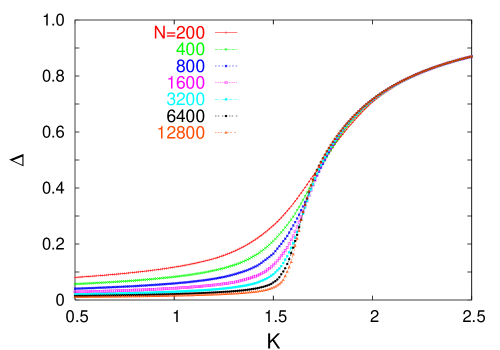
Figure 1: Phase synchronization order parameter $\Delta$ versus the coupling strength $K$ for various system sizes $N$.

To pin down the transition point $K_{c}$ precisely, we use the Binder cumulant method ref:BC1 ; ref:BC11 . The fourth-order cumulant of the order parameter, the Binder cumulant (BC), is defined in thermal systems as

$$B_{\Delta}=1-\frac{\langle\Delta^{4}\rangle}{3\langle\Delta^{2}\rangle^{2}},$$ (6)

where $\langle\cdots\rangle$ represents the thermal (time) average. In systems with quenched disorder, on the other hand, we should consider the disorder average besides the thermal one. We may first consider the BC as the disorder-averaged moment ratio ref:BC2 ; ref:BC5 ; ref:SG

$$B_{\Delta}^{(1)}=1-\frac{[\langle\Delta^{4}\rangle]}{3[\langle\Delta^{2}\rangle]^{2}},$$ (7)

where $[\cdots]$ denotes the disorder average, i.e., the average over different realizations of $\{\omega_{i}\}$.

Figure 2 displays $B_{\Delta}^{(1)}$ as a function of the coupling strength $K$ for various system sizes $N$. In the region of weak coupling $(K\rightarrow 0)$, we expect the random nature of the oscillator phases $\{\phi_{i}\}$ to yield an asymmetric Poisson-like probability distribution function (PDF) characterized by $P(\Delta)\sim\Delta\exp(-c\Delta^{2})$ with a constant $c$, which leads to $B_{\Delta}^{(1)}=1/3$. On the other hand, in the strong-coupling region, the PDF becomes a $\delta$-like function with a very narrow variance, which leads to $B_{\Delta}^{(1)}=2/3$. The numerical data in Fig. 2 are consistent with our predictions.

However, near the transition, the $B_{\Delta}^{(1)}$ shows a big anomalous “dip” on the desynchronized side. As the system size increases, the dip develops initially with a broad width and then becomes sharper and also deeper. The dip’s position moves toward the transition point. The crossing points seem to nicely converge to the critical point $K_{c}=\sqrt{8/\pi}$. However, as the system size increases, the presence of the dip starts to hinder us in locating the critical point accurately.

In this Letter, we explain why the dip develops in this system and propose alternative definitions of the Binder cumulant that do not show any dip in the same system. We measure the disorder (sample-to-sample) fluctuations defined as

$$A_{\cal O}=\frac{[\langle{\cal O}\rangle^{2}]}{[\langle{\cal O}\rangle]^{2}}-1,$$ (8)

where ${\cal O}$ is any observable, such as $\Delta$ and $\Delta^{2}$, in a system. This quantity is positive definite and is supposed to vanish in the thermodynamic limit in self-averaging systems and to remain finite in non-self-averaging systems ref:NSA ; ref:SG . As one can see in Fig. 3, the disorder fluctuation $A_{\Delta^{2}}$ is quite sizable in the range of $K$ where the dip appears ($A_{\Delta}$ shows a similar behavior). In other words, the $B_{\Delta}^{(1)}$ shows a dip where the system is not well self-averaged. A careful finite-size analysis on $A_{\Delta^{2}}$ reveals that it vanishes as $\sim N^{-1}$ away from criticality, but saturates to a finite value at criticality. The non-self-averageness at criticality is not surprising because the quenched randomness in natural frequencies should be relevant at this transition.

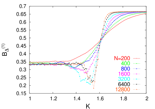
Figure 2: Binder cumulant $B^{(1)}_{\Delta}$, defined by Eq. (7), of the phase synchronization order parameter $\Delta$.

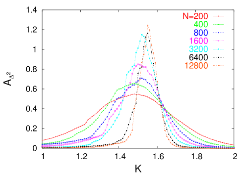
Figure 3: Disorder fluctuation $A_{\Delta^{2}}$ defined by Eq. (8).

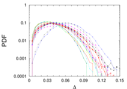
Figure 4: Probability distribution function (PDF) at $K=1.5$ and $N=12800$ in the steady state. Each curve corresponds to one of 20 independent samples.

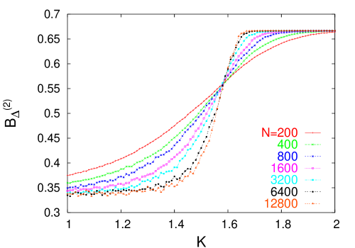
Figure 5: Binder cumulant $B^{(2)}_{\Delta}$ defined by Eq. (9). Note that the dip shown in $B^{(1)}_{\Delta}$ disappears.

Strong disorder fluctuations may cause non-negligible spreading of the effective coupling constants over different realizations of disorder ref:NSA . Figure 4 shows for 20 independent samples, the PDF of $\Delta$ just below the transition and obtained from the time series of $\Delta$ after the system had reached the steady state. Indeed, a large part of the sample-to-sample variations can be interpreted as a shift in the $K_{c}$ of individual samples. The two quantities ${[\langle\Delta^{2}\rangle]}$ and $[\langle\Delta^{4}\rangle]$ in Eq. (7) can be considered as the second and the fourth moments of the disorder-averaged PDF, which is much broader than the individual PDFs near the transition. One can easily see that broadening yields a larger value for the ratio $[\langle\Delta^{4}\rangle]/[\langle\Delta^{2}\rangle]^{2}$ and, hence, a smaller BC. The effect is particularly pronounced on the small $K$ side of the transition, where $\Delta$ itself is small, in which case a shift in $K_{c}$ has a stronger influence on the moments.

An alternative definition for the Binder cumulant for systems with quenched disorder (especially non-diminishing disorder fluctuations) isref:QS ; ref:HH

$$B^{(2)}_{\Delta}=1-\Biggl{[}\frac{\langle\Delta^{4}\rangle}{3\langle\Delta^{2}\rangle^{2}}\Biggr{]}.$$ (9)

We note that the disorder average is performed over the ratio of the time-averaged moments. The moment ratio is calculated for each sample first and, is then averaged over disorder. It is clear that this definition of the Binder cumulant should eliminate the most dominant contribution from the disorder fluctuations, i.e., the anomaly caused by the spreading of the effective coupling constants. This definition has been adopted mostly in quantum disorder systems, where strong disorder fluctuations are anticipated ref:QS . Figure 5 displays $B^{(2)}_{\Delta}$ versus $K$. We note that the dip shown in Fig. 2 disappears and that the crossing points nicely converge to $K_{c}$, implying that $B^{(2)}_{\Delta}$ should serve better for locating the transition point than the conventional one, which is confirmed numerically (not shown here).

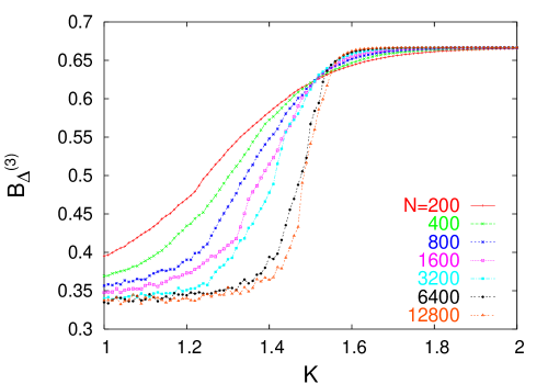
Figure 6: Binder cumulant $B^{(3)}_{\Delta}$ defined by Eq. (10).

Yet another definition of the Binder cumulant is

$$B_{\Delta}^{(3)}=1-\frac{[\langle\Delta^{4}\rangle]}{3[\langle\Delta^{2}\rangle^{2}]}.$$ (10)

We expect that $B_{\Delta}^{(3)}$ may also behave smoothly near the transition because it does not involve disorder fluctuation terms such as $[\cdots]^{2}$ included in $B_{\Delta}^{(1)}$. Figure 6 displays $B^{(3)}_{\Delta}$ versus $K$. As expected, we find no anomalous behavior in $B_{\Delta}^{(3)}$. We can directly relate $B_{\Delta}^{(1)}$ and $B_{\Delta}^{(3)}$ through the disorder fluctuation $A_{\Delta^{2}}$. Simple algebra leads to

$$B^{(1)}_{\Delta}=B^{(3)}_{\Delta}-(1-B^{(3)}_{\Delta})A_{\Delta^{2}}.$$ (11)

As the disorder fluctuation $A_{\Delta^{2}}$ becomes larger, $B^{(1)}_{\Delta}$ shows a bigger dip. This explains quantitatively the size and the location of the dip in $B^{(1)}_{\Delta}$. The critical value of $B^{(3)}_{\Delta}$ ($\approx 2/3$) provides additional information on the temporal variations of $\Delta$. One can show that $3B^{(3)}_{\Delta}=2-[\langle\delta\Delta^{2}\rangle]/[\langle\Delta^{2}\rangle^{2}]$, where $\langle\delta\Delta^{2}\rangle=\langle\Delta^{4}\rangle-\langle\Delta^{2}\rangle^{2}$. Our numerical result indicates that the relative temporal fluctuations are almost negligible even at criticality. In this case, $B^{(3)}_{\Delta}$ is not practically useful in locating the transition point accurately.

In summary, we studied Binder cumulants in the quenched disorder system. For the Kuramoto model, we found that the conventionally defined BC shows a big anomalous dip near the transition. This dip is shown to be directly related to the disorder fluctuation (non-self-averageness). Alternative definitions of the BC, which did not show any anomalous behavior were proposed and may be useful in locating the transition point accurately in general systems with quenched disorder.

References

- (1) K. Binder, Z. Phys. B 43, 119 (1981); Phys. Rev. Lett 47, 693 (1981).
- (2) K. Binder, in Finite-Size Scaling and Numerical Simulation of Statistical Systems, edited by V. Privman (World Scientific, Singapore, 1990), p. 173; K. Binder and D. W. Heermann, Monte Carlo Simulation in Statistical Physics. An Introduction, 3rd ed. (Springer, Berlin, 1997).
- (3) R. N. Bhatt and A. P. Young, Phys. Rev. Lett. 54, 924 (1985); Phys. Rev. B 37, 5606 (1988); N. Kawashima and A. P. Young, Phys. Rev. B 53, R484 (1996).
- (4) X. S. Chen and V. Dohm, Phys. Rev. E 70, 056136 (2004); W. Selke, Eur. Phys. J. B 51, 223 (2006).
- (5) M. Acharyya, Phys. Rev. E 59, 218 (1999); G. Korniss, P. A. Rikvold, and M. A. Novotny, Phys. Rev. E 66, 056127 (2002).
- (6) K. Hukushima and H. Kawamura, Phys. Rev. E 62, 3360 (2000); T. Shirakura and F. Matsubara, Phys. Rev. B 67, 100405(R) (20003).
- (7) Y. Kuramoto, in Proceedings of the International Symposium on Mathematical Problems in Theoretical Physics, edited by H. Araki (Springer-Verlag, New York, 1975); Y. Kuramoto, Chemical Oscillations, Waves, and Turbulence (Springer-Verlag, Berlin, 1984); Y. Kuramoto and I. Nishikawa, J. Stat. Phys. 49, 569 (1987).
- (8) C. Pich, A. P. Young, H. Rieger, and N. Kawashima, Phys. Rev. Lett. 81, 5916 (1998); R. Sknepnek, T. Vojta, and M. Vojta, Phys. Rev. Lett. 93, 097201 (2004).
- (9) H. Hong, H. Park, and M. Y. Choi, Phys. Rev. E 70, 045204(R) (2004); Phys. Rev. E 72, 036217 (2005).
- (10) H. Hong, H. Chaté, H. Park, and L.-H. Tang (in preparation).
- (11) See, e.g., R. L. Burden and J. D. Faires, Numerical Analysis (Brooks/Cole, Pacific Grove, 1997), p. 280.
- (12) A. Billoire and B. Coluzzi, Phys. Rev. E 68, 026131 (2003); G. Parisi, M. Picco, and F. Ritort, Phys. Rev. E 60, 58 (1999); M. Picco, F. Ritort, and M. Sales, Eur. Phys. J. B 19, 565 (2001).
- (13) S. Wiseman and E. Domany, Phys. Rev. Lett. 81, 22 (1998); Phys. Rev. E 52, 3469 (1995); A. Aharony and A. B. Harris, Phys. Rev. Lett. 77, 3700 (1996).
- (14) J. Houdayer and A. K. Hartmann, Phys. Rev. B 70, 014418 (2004); J. D. Noh, H. Rieger, M. Enderle, and K. Knorr, Phys. Rev. E 66 , 026111 (2002).