The Effect of Quantum Phase Slip Interactions on the Transport of Thin Superconducting Wires

Abstract

We study theoretically the effect of interactions between quantum phase slips in a short superconducting wire beyond the dilute phase slip approximation. In contrast to the smooth transition in dissipative Josephson junctions, our analysis shows that treating these interactions in a self consistent manner leads to a very sharp transition with a critical resistance of $R_{Q}=h/(4e^{2})$. The addition of the quasi-particles resistance at finite temperature leads to a quantitative agreement with recent experiments on short MoGe nanowires. Our treatment is complementary to the theory of the thermal activation of phase slips, which is only valid for temperature at the vicinity of the mean field metal to superconductor transition. This self consistent treatment should also be applicable to other physical systems that can be mapped onto similar sine-Gordon models, in the intermediate-coupling regime.

One of the most intriguing problems in low-dimensional superconductivity is the understanding of the mechanism that drives the superconductor-insulator transition (SIT). Experiments conducted on quasi-one-dimensional (1D) systems have shown that varying the resistances and diameters of thin metallic wires can suppress superconductivity PXiongPRL1997 ; YOregPRL1999 , and in certain cases lead to an insulating-like behavior FSharifiPRL1993 ; ABezryadinNAT2000 ; CNLauPRL2001 ; ATBollinger2005 . We focus on recent experiments conducted on short ultrathin MoGe nanowires ATBollinger2005 that show a SIT driven by the wires’ normal state resistance with a critical resistance $R_{c}\approx R_{Q}$.

The universal critical resistance may suggest that at a temperature much lower than the mean field transition temperature, $T\ll T_{c}$, the wire acts as a superconducting (SC) weak link resembling a Josephson junction (JJ) connecting two superconducting leads. Schmid ASchmidPRL1983 and Chakravarty SChakravartyPRL1982 showed that a JJ undergoes a SIT as a function of the junction’s shunt resistance, $R_{\textrm{s}}$, with a critical resistance of $R_{Q}$, and that the temperature dependence of the resistance obeys the power law $R(T)\propto T^{2\left(\frac{R_{Q}}{R_{\textrm{s}}}-1\right)}$. The theory was later extended to JJ arrays and SC wires HPBuchlerPRL2004 ; GRefael2005 ; GRefael2006 . Within these theories, a similar power-law temperature dependence of the resistance at low temperature prevails.

A power-law $R(T)$ implies a rather wide SIT, with a resistance that has only a weak temperature dependence in the critical region. Contrary to the theoretical analogy with a single JJ, A. T. Bollinger et al. ATBollinger2005 observe that the resistance of quasi 1D MoGe nanowires exhibits a strong temperature dependence, even close to the SIT. In fact, the resistance could be fitted with a modified LAMH theory JSLangerPR1967 ; DEMcCumberPRB1970 of thermally activated phase slips down to very low temperatures. Nevertheless, for these narrow wires it appears that the LAMH theory is valid only in a narrow temperature window CommentLAMHValidity ; RSNewbowerPRB1972 . Moreover, the LAMH analysis does not explain the appearance of the universal critical resistance $R_{Q}$.

In this manuscript we propose an approach that captures both the universal critical resistance at the SIT, and the sharp decay of the resistance as a function of temperature. As in previous works, we treat the SIT in nanowires as a transition governed by quantum phase-slip (QPS) proliferation. This picture alone, however, cannot account for the observed strong temperature dependence of the resistance. We claim that the key ingredient left out in previous works is the inclusion of interactions between phase slips in the finite-size wire, when the phase-slip population is dense - a situation that occurs in thin wires at high temperatures (see also Ref. GRefael2006 ).

We treat these interactions in a mean-field type approximation: when analyzing the behavior of a small segment of the wire, we include in its effective shunt-resistance the resistance due to phase slips elsewhere in the wire. This scheme is motivated by numerical analysis of a related problem, an interacting pair of resistively-shunted JJs PWernerJSM2005 . Primarily, this self-consistent treatment produces the sharp temperature dependence of the resistance. In addition, we include the effects of the Bogoliubov quasi-particles, which couple to the potential gradient created by each phase-slip CommentBdGQuasiParticles . Consequently, the resistance obtained in the experiment can be fitted without resorting to the LAMH theory beyond its limit of validity. This self-consistent approximation of phase-slip interactions should be applicable to similar multiple sine-Gordon models in the intermediate-coupling regime.

The microscopic action for a SC wire can be obtained from the BCS Hamiltonian by a Hubbard-Stratanovich transformation followed by an expansion around the saddle point CommentDirtyLimit . In the limit of low energy scales, $\omega,Dq^{2}~{}\ll~{}\Delta_{0}$, this yields DSGolubevPRB2001 :

$$S = N_{0}A\Delta_{0}^{2}\int_{0}^{L}dx\int_{0}^{1/T}d\tau\left\{\frac{\rho^{2}}{2}\left[\ln\left(\rho^{2}\right)-1\right]\right.$$ (1)

$$\left.+2\xi_{0}^{2}\rho^{2}\left[\phi^{\prime 2}+\frac{1}{v_{\phi}^{2}}\dot{\phi}^{2}\right]+\xi_{0}^{2}\left[\rho^{\prime 2}+\frac{1}{v_{\rho}^{2}}\dot{\rho}^{2}\right]\right\},$$

where $L$ and $A$ are the wire’s length and cross section, respectively, $\xi_{0}^{2}=\pi D/8\Delta_{0}$, $v_{\rho}=\sqrt{(3\pi/2)D\Delta_{0}}$ the amplitude velocity, $v_{\phi}=\sqrt{\pi D\Delta_{0}(2AV_{c}N_{0}+1)}$ the phase velocity, $V_{c}$ the Fourier transform of the short range Coulomb interaction, $N_{0}$ the density of states, $D$ the electronic diffusive constant in the normal state, and the SC order parameter is parameterized as $\Delta=\Delta_{0}\rho e^{i\phi}$, with $\Delta_{0}$, the mean field solution. For the wires in Ref. ATBollinger2005, $2AV_{c}N_{0}\propto N_{\bot}\gg 1$, leading to $v_{\rho}\ll v_{\phi}\propto v_{\rho}\sqrt{N_{\bot}}$. Here $N_{\bot}=p_{F}^{2}A/\pi^{2}$ is the number of 1D channels in the wire.

This action supports QPS excitations, which are characterized by two distinct length scales: $v_{\rho}/\Delta_{0}\propto\xi\ll\xi\sqrt{N_{\bot}}\propto v_{\phi}/\Delta_{0}$. For very long wires, $\xi\ll\xi\sqrt{N_{\bot}}\ll L$, in the dilute phase slip approximation, this problem can be mapped onto the perturbative limit of the $1+1$ sine-Gordon model HPBuchlerPRL2004 . In the opposite limit of very short wires, $L<\xi\ll\xi\sqrt{N_{\bot}}$, the system resembles a JJ and can be mapped onto the $0+1$ sine-Gordon model. However the MoGe nanowires in Ref. ATBollinger2005, appear to be in the intermediate regime, $\xi\ll L\ll\xi\sqrt{N_{\bot}}$. Hence, while phase slips occur in different sections of the wire, they are indistinguishable, as each creates a phase fluctuation that spreads over distances larger than the wire itself.

Moreover, the wires in Ref. ATBollinger2005 have a sizable bare fugacity. Using Eq. (1), one can estimate the core action of a phase slip of duration $\tau_{0}=1/\Delta_{0}$ by minimizing the action with respect to the diameter of a phase slip CommentCoreAction ; RSmithUnPublished . This yields a core action of $S_{c}=\pi/8\sqrt{1/3(1-\epsilon)}R_{Q}/R_{\xi}$. Here $\epsilon=1-T/T_{c}$ is the reduced temperature and $R_{\xi}=R_{\textrm{W}}\xi/L$ is the normal resistance of a section of length $\xi$. With this expression, the measured values of $R_{\textrm{W}}$ and $L$ (Table 1), and the assumption that $\xi\approx 20nm$, the phase slip fugacity is estimated by $\zeta=e^{-S_{c}}\approx 0.05-0.45$, for the different wires. Namely, in the critical region, $R_{\textrm{W}}\approx R_{Q}$, there is a dense population of phase slips which interact with one another; thus the dilute phase slip approximation is no longer a proper description.

The flow equation for the fugacity of a phase slip anywhere in the wire is given by:

$$d\zeta/dl = \left(1-R_{Q}/R_{\textrm{s}}\right)\zeta,$$ (2)

where $dl=-d\ln\Lambda$, and $\Lambda$ is the running RG scale. Eq. (2) treats the phase slip as occuring on an effective JJ, with $R_{\textrm{s}}$ being the effective shunting resistance of the entire wire. When $\zeta$ is small, $R_{\textrm{s}}$ will include only the effective impedance of the leads. If $\zeta$ is not very small, we will need to include in Eq. (2) additional terms of higher powers of $\zeta$, which describe interactions between QPSs. Currently, there is no complete understanding of how to approach the field theory of phase slips in the regime of intermediate fugacity $\zeta\lesssim 1$. Therefore, we suggest to take into account a finite $\zeta$ by including the resistance due to other phase slips in the wire in the effective shunt resistance of the junction, $R_{\textrm{s}}$. This treatment was successfully tested by numerical analysis of a simpler analog of the system, an interacting pair of resistively shunted JJs PWernerJSM2005 . Indeed, including the interaction between phase slips as a modification of the shunt, $R_{\textrm{s}}$, is akin to guessing the form of a complete resummation of higher-order $\zeta$ terms in Eq. (2) CommentNextOrderInRG ; BulgadaevPLA1981 .

The main physical intricacy is the determination of the effective shunt resistance, $R_{\textrm{s}}(\zeta)$, that governs the renormalization of the phase slip fugacity [Eq. (2)]. A phase slip produces time-varying phase gradients, and hence electrical fields. These dissipate through two channels in parallel: the SC channel - which has an effective resistance due to other phase slips, $R_{\textrm{{ps}}}$ - and the quasi-particles conducting channel CommentBdGQuasiParticles , $R_{\textrm{{qp}}}$. Once the disturbance reaches the leads, it also dissipates through the electro-dynamical modes of the large electrodes, whose real impedance is parameterized by $R_{\textrm{{elec}}}$.

For $T\ll~{}T_{c}$, the resistance of the quasi particles, $R_{\textrm{{qp}}}$, can be approximated by $R_{\textrm{{qp}}}=\frac{m}{e^{2}\tau_{\textrm{n}}n_{\textrm{{qp}}}}\frac{L}{A}=R_{\textrm{n}}\frac{n}{n_{\textrm{{qp}}}}\approx R_{\textrm{n}}\sqrt{\frac{T}{2\pi\Delta_{0}}}e^{\frac{\Delta_{0}}{T}}$. Unfortunately, we lack a microscopic model for the impedance of the electrodes, as this depends on the details of the system. However, we expect that at large scales, $T<\Lambda<\Delta$, the electrodes will act as a transmission line to the electromagnetic waves generated by the phase slip. This transmission line is characterized by a real impedance which we denote as $R_{\textrm{{elec}}}$, and use as a fitting parameter. Hence, the effective shunt resistance that affects the renormalization of the phase slip fugacity at $T<\Lambda<\Delta$ [Eq. (2)] is

$$R_{\textrm{s}}[\zeta(\Lambda)]=R_{\textrm{{elec}}}+1/\left(1/R_{\textrm{{ps}}}[\zeta(\Lambda)]+1/R_{\textrm{{qp}}}(T)\right).$$ (3)

Fig. 1 shows the circuit we suggest describes the system.

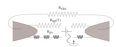
Figure 1: The effective electrical circuit for the nanowire. A phase slip produces time-varying phase gradients, and hence electrical fields, that dissipate through the quasi-particles conducting channel, $R_{\textrm{{qp}}}$, and through the SC channel, that has an effective resistance due to other phase slips, $R_{\textrm{{ps}}}$. Once the disturbance reaches the edges, it also dissipates through the electro-dynamical modes of the large electrodes, whose real impedance is represented by $R_{\textrm{{elec}}}$.

The resistance is measured in response to an applied DC current. At this zero frequency limit, the electrodes act as a capacitor connected in parallel to the wire. Therefore, the measured resistance is the total wire resistance, unaffected by the environment, which is cut off from the wire.

$$R_{\textrm{{tot}}}(T)=1/\left(1/R_{\textrm{{ps}}}[\zeta(T)]+1/R_{\textrm{{qp}}}(T)\right).$$ (4)

The occurrence of a phase slip causes a resistance in the otherwise SC wire through the relation $R_{\textrm{{ps}}}\propto(L/\xi)\zeta^{2}$. Using this relation and Eq. (2), we can write an RG equation for the dimensionless resistance

$$\frac{d\zeta^{2}}{dl} = 2\zeta\frac{d\zeta}{dl}=2\left(1-\frac{R_{Q}}{R_{\textrm{{s}}}(\zeta)}\right)\zeta^{2}$$

$$\Rightarrow\frac{d\left(R_{\textrm{{ps}}}/R_{Q}\right)}{dl} = 2\left(1-\frac{R_{Q}}{R_{\textrm{{s}}}(R_{\textrm{{ps}}})}\right)\left(\frac{R_{\textrm{{ps}}}}{R_{Q}}\right).$$ (5)

If we now substitute the effective resistance in Eq. (3), depicted in Fig. 1, into the RG equation (The Effect of Quantum Phase Slip Interactions on the Transport of Thin Superconducting Wires), we find the following self consistent equation:

$$\frac{d\left(\frac{R_{\textrm{{ps}}}}{R_{Q}}\right)}{dl} = \!\!2\!\!\left[1-\frac{R_{Q}}{\left(R_{\textrm{{elec}}}+\frac{R_{\textrm{{ps}}}R_{\textrm{{qp}}}(T)}{R_{\textrm{{ps}}}+R_{\textrm{{qp}}}(T)}\right)}\right]\!\!\left(\frac{R_{\textrm{{ps}}}}{R_{Q}}\right).$$ (6)

Integrating Eq.(6) from the ultra violet (UV) cutoff, $\Delta(T^{*})=T^{*}$, to the infra red cutoff, $T$, yields $R_{\textrm{{ps}}}(T)$.

The wire’s DC resistance Eq. (4), calculated using Eq. (6), is plotted in Fig 2 as a function of temperature for different $R^{*}$. Here $R^{*}\equiv R_{\textrm{{tot}}}(T^{*})$ is the normal state resistance of the wire, at the UV cutoff $\Delta(T^{*})=T^{*}$. We assume that the wires are thin enough such that the mean field transition from normal to SC is wide, and $R^{*}\approx R_{\textrm{{tot}}}(T_{c}^{+})=R_{\textrm{n}}$. For simplicity, we have assumed throughout our calculation that $\Delta(T)\approx\Delta$. This assumption holds at the low temperature regime, $T\ll\Delta$, where the theory of QPSs, based on the effective action Eq. (1), is expected to be valid. The resistance of the environment is taken to be $R_{\textrm{{elec}}}=0.1R_{Q}$. In practice, $\Delta$, $R^{*}$ and $R_{\textrm{{elec}}}$ can be used as fitting parameters, when comparing the theory to the experiment. Moreover, $R^{*}$ can be determined independently as the resistance measured below the drop that indicates passing through $T_{c}$ of the SC films (see Ref. ATBollinger2005, ).

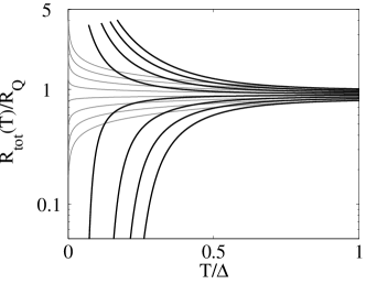
Figure 2: Reduced resistance $R_{\textrm{{tot}}}/R_{Q}$ as a function of renormalized temperature $T/\Delta$ for different $R^{*}/R_{Q}$, ranging from $0.8$ (lower plot) to $1.01$ (upper plot) in increasing steps of $0.03$. The environment resistance was taken to be $R_{\textrm{{elec}}}/R_{Q}=0.1$. Gray traces indicate the total wire resistance $R_{\textrm{{tot}}}=\frac{R_{\textrm{{ps}}}R_{\textrm{{qp}}}(T)}{R_{\textrm{{ps}}}+R_{\textrm{{qp}}}(T)}$, with $R_{\textrm{{ps}}}(T)=R^{*}\left(T/\Delta\right)^{2(R_{Q}/R_{\textrm{s}}-1)}$, and constant $R_{s}=R^{*}+R_{\textrm{{elec}}}$. The insulating plots are cutoff at temperature, $T_{0}$, for which $\zeta(T_{0})=1$.

Eq. (6) is also applicable to a wire with a normal resistance larger than the quantum resistance, $R^{*}>R_{Q}$. In this limit the fugacity increases in the renormalization process, and Eq. (2) is no longer valid for $\zeta\gtrsim 1$. For wires with $R^{*}>R_{Q}$, we overestimate the phase slip fugacity as $\zeta(T^{*})=0.5$, and plot the reduced resistance, $R_{\textrm{{tot}}}/R_{Q}$, down to the temperature, $T_{0}$, for which $\zeta(T_{0})=1$. The results are shown in Fig. 2. Overestimating $\zeta(T^{*})$ gives an upper bound on $T_{0}$, where Eq. (2) is no longer applicable. Fig. 2 shows that the transition between SC and insulating wires occurs for a critical resistance $R_{c}\approx R_{Q}$. But in contrast to the standard Josephson junction theory, (gray curves in Fig. 2), the transition is much more sharp (notice the $\log$ scale).

	Measured Values			Fitting Values
Curve	$L(nm)$	$R_{\textrm{W}}(k\Omega)$		$R^{*}(k\Omega)$		$\Delta(K)$		$R_{\textrm{{elec}}}(k\Omega)$
$1$	177	005.	46	004.	2	02.	5	001.	2
$2$	43	3.	62	2.	62	2.	35	1.	25
$3$	63	2.	78	2.	13	3.	07	0.	66
$4$	93	3.	59	2.	89	3.	85	0.	55
$5$	187	4.	29	4.	5	6.	55	0.	31
$6$	99	2.	39	2.	09	4.	84	0.	4

Table 1: Summary of nanowire parameters, and the parameters used to fit the experimental data; $L$ is the length of the wire determined from SEM images, $R_{\textrm{W}}$ is the wire’s normal state resistance, taken as the resistance measured below the film transition. Fitting parameters: $R^{*}=R_{\textrm{tot}}(T=\Delta)$ is the wire’s resistance at the UV cutoff, $\Delta$ the SC order parameter, and $R_{\textrm{{elec}}}$ the impedance of the electrodes at $T<\Lambda<\Delta$.

A comparison between the theoretical curves and the experimental data taken from Ref. ATBollinger2005, is shown in Fig.  3. The curves were calculated by fitting $R^{*}$, $\Delta$, and $R_{\textrm{{elec}}}$. Since the theory of QPSs is expected to be valid at $T\ll\Delta$, deviations from the theoretical curves at high temperature are reasonable. In general, as $\Delta$ is proportional to $T_{c}$, increasing $\Delta$ shifts the sharp decay of the resistance to high temperatures. Both $R^{*}$ and $R_{\textrm{{elec}}}$ affect the high temperature resistance, whereas $R^{*}$ and $\Delta$ control the width of the transition.

We have made an attempt to fit the experimental data corresponding to the insulating wires of Ref. ATBollinger2005, . As the insulating wires are thinner, we expect a strong suppression of $T_{c}$ YOregPRL1999 . Consequently, the theory of QPSs with $\zeta\lesssim 1$, is valid in a narrow range of temperatures. While we manage to fit the experimental curves in this regime of parameters, we do not find it of scientific merit to present the results (our fits cover a range of $\sim 10$ data points, with three fitting parameters).

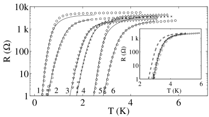
Figure 3: Comparison between the theory (solid line) and the experimental data ATBollinger2005 . Details of the wires, as well as fitting parameters are summarized in Table 1. Note that the estimated values for $R^{*}$ are in good agreement with the measured values of the resistance of the wire at $T=\Delta$. The discrepancies between theory and experiment occur for the longer wires (curves $1$ and $5$). In these wires the condition $v_{\phi}/\Delta_{0}\gg L$ might not hold, and one should consider additional renormalization of the fugacity at higher scales. Inset: The effect of an adjustment of the fit parameters, in roughly $10\%$ (from dark gray to light gray): $\Delta=4.356K$, $R_{\textrm{{elec}}}=440\Omega$ and $R^{*}=1881\Omega$.

In conclusion, we have studied theoretically the effect of interactions between QPSs, in short SC wires, beyond the dilute phase slip approximation. Our analysis shows that treating these interactions in a self consistent manner, produces a sharp SIT transition, with a critical resistance $R_{c}\approx R_{Q}$, in agreement with recent experiments conducted on short ultrathin MoGe nanowires ATBollinger2005 . Moreover, we have shown that adding the resistance due to the presence of a finite number of BdG quasi-particles in the wire leads to a quantitative agreement with the experimental curves. Our method should be applicable to a wider range of physical problems which involve the proliferation of topological defects with a sizable bare fugacity. In particular, it could be applied to the study of a Luttinger liquid with an extended impurity CLKanePRB1992 .

We would like to thank E. Demler, R. A. Smith, and P. Werner. Special thanks to A. Bezryadin for making his data available to us. This study was supported by a DIP grant.

References

- (1) P. Xiong, A. V. Herzog, and R. C. Dynes, Phys. Rev. Lett. 78, 927 (1997).
- (2) Y. Oreg and A. M. Finkel’stein, Phys. Rev. Lett. 83, 191 (1999).
- (3) F. Sharifi, A. V. Herzog, and R. C. Dynes, Phys. Rev. Lett. 71, 428 (1993).
- (4) A. Bezryadin, C. N. Lau, and M. Tinkham, Nature 404, 971 (2000).
- (5) C. N. Lau, N. Markovic, M. Bockrath, A. Bezryadin, and M. Tinkham, Phys. Rev. Lett. 87, 217003 (2001).
- (6) A. T. Bollinger, A. Rogachev, and A. Bazryadin, condmat , 0508300 (2005).
- (7) A. Schmid, Phys. Rev. Lett. 51, 1506 (1983).
- (8) S. Chakravarty, Phys. Rev. Lett. 49, 681 (1982).
- (9) H. P. Büchler, V. B. Geshkenbein, and G. Blatter, Phys. Rev. Lett. 92, 067007 (2004).
- (10) G. Refael, E. Demler, Y. Oreg, and D. S. Fisher, condmat , 0511212 (2005).
- (11) G. Refael, E. Demler, and Y. Oreg, In preparation.
- (12) J. S. Langer and V. Ambegaokar, Phys. Rev. 164, 498 (1967).
- (13) D. E. McCumber and B. I. Halperin, Phys. Rev. B 1, 1054 (1970).
- (14) The LAMH theory of thermally activated phase slips is based on the time dependent Ginzburg-Landau (TDGL) description of a superconducting wire. This description is valid at temperatures higher than the gap, and far enough from , such that fluctuation corrections can be ignored, . Here is defined by , with the temperature dependent order parameter, and , with the Ginzburg-Levanyuk number for the quasi 1D wires. Here is the normal resistance of a section of length . For the wires in Ref. ATBollinger2005, , the applicability of LAMH is marginal as , and estimates for range between and (see Table 1). These estimates should be contrasted with the well established fit of the LAMH theory to tin whisker crystals RSNewbowerPRB1972 , where the theory is applicable for , and the range of fitting was . Here is the reduced temperature.
- (15) R. S. Newbower, M. R. Beasley, and M. Tinkham, Phys. Rev. B 5, 864 (1972).
- (16) P. Werner, G. Refael, and M. Troyer, J. Stat. Mech. , P12003 (2005).
- (17) This could be seen by considering a time dependent Bogoliubov de Gennes (BdG) equation, with a time dependent phase: . By the canonical transformation , we produce an effective potential for the quasi-particles in the BdG Hamiltonian.
- (18) The expansion is done in the dirty limit, , where is the scattering mean free time.
- (19) D. S. Golubev and A. D. Zaikin, Phys. Rev. B 64, 014504 (2001).
- (20) To estimate the core action, we choose the following trial function for a phase slip: , and . Identifying the part of the action [Eq. (1)], that corresponds to as the core action, we minimize this expression with respect to the phase slip diameter, . Keeping only leading terms in , one finds .
- (21) Robert A. Smith and Yuval Oreg (unpublished).
- (22) For instance, adding the next order term, , BulgadaevPLA1981 to Eq. (2), can be thought of as modifying by . .
- (23) S. A. Bulgadaev, Phys. Lett. A 86, 213 (1981).
- (24) C. L. Kane and M. P. A. Fisher, Phys. Rev. B 46, 15233 (1992).