Exactly solvable model of electron in the Lame potential
and singularities of the electron thermodynamic potential

Abstract

One-gap and two-gap separable Lame potentials are studied in detail. For the one-dimensional case, we construct the dispersion relation graph $E(k)$ and for the three-dimensional case we construct the Fermi surfaces in the first and second bands. The pictures illustrate a passage from the limit case of free electrons to the limit case of tight binding electrons. These results are used to describe the Lifshits electron phase transition of $2\frac{1}{2}$ kind and derive some exact expressions. We also examine the singularities of the second derivative of magnetic momentum in an external magnetic field. The parameter of the singularities depends on corresponding effective mass.

I Introduction

There is a sufficient number of numerical and self-consistent methods to compute the one particle spectrum of a solid with good accuracy. However, in addition to this, it is desirable to have analytical solutions of the Schrödinger equation. These solutions for multidimensional periodic potentials are useful both for a zero order perturbation theory and for the general theory. This allows us, for example, to gain a deeper understanding of spectral manifolds and corresponding eigenfunctions, as well as their geometrical and analytical properties.

Among one-dimensional potentials, the finite-gap ones are the most interesting and fruitful in the view of the physical results. The Schrödinger equation with the finite-gap potential ZMNP ; BBEIM has an exact solution, the spectrum and eigenfunctions are defined by analytical functions.

The Kronig-Penny potential KP consisting of rectangular wells is usually considered as the most elementary one in the quantum physics of solids. However, in order to determine the band structure that corresponds to this potential, it is necessary to solve transcendental equation and, furthermore, the appropriate eigenfunctions are too cumbersome to use them to calculate the matrix elements of any observables. The finite-gap potentials are free of these limitations. The matrix elements of any observable on the eigenfunctions that correspond to finite-gap potential can be calculated analytically by the residue method. Furthermore, one can say that these potentials play the same role in solid-state physics as the Kepler problem plays in atomic theory.

It is known that generic periodic potential has generally an infinite set of gaps in the spectrum, but their width rapidly decreases as energy increases. If a potential is analytical, then the rate of decrease is exponential. Therefore, provided narrow enough gaps in the spectrum are disregarded, any periodic potential can be approximated by a finite-gap potential. MO It turns out also that the finite-gap potentials are exact solutions of the Peierls-Fröhlich problem on a self-consistent state of the lattice and conduction electrons. B

The simplest finite-gap potentials are the Lame ones. I ; I1 ; BEES ; T They are expressed through the Weierstrass function. The Lame potentials are a subset of the Darboux potentials, D that are linear superpositions of the Weierstrass functions with half-period shifts. Whatever the number of gaps, all these potentials are characterized by only two parameters of the elliptic function. Treibich and Verdier rediscovered the Darboux potentials and described them in algebraic-geometric terms of the tangent covers and studied their spectral properties. T1 ; TV ; TV1 Krichever suggested considering elliptic finite-gap potentials from the point of view a torus covering. K Using this approach, Smirnov has presented a large list of these potentials. S Its and Matveev derived a general formula that expresses an arbitrary finite-gap potential through the multidimensional Riemann $\theta$-functions, the parameter number of which coincides with the number of band edges. IM

There are also multidimensional elliptic Calogero-Moser potentials, which their integrability was proved by Olshanetsky and Perelomov. OP

Baryakhtar, Belokolos and Korostil suggested considering the Schrödinger equation with three-dimensional separable potential as a sum of three one-dimensional finite-gap potentials along orthogonal directions. BBK2 It is obvious that these potentials correspond to the orthorhombic lattice. The Schrödinger equation with such a potential has the exact eigenfunctions and the spectrum is defined by analytical functions. The parameters that this model includes have simple physical sense. These parameters are related to the width of spectral gaps. As an example, let us consider separable elliptic finite-gap potentials. The Weierstrass function has two independent parameters: the parameter $\omega^{\prime}$ defines the potential period, the parameter $\omega$ defines the gap width along corresponding direction of dual lattice. It is natural to consider the parameter $\tau={\omega^{\prime}}/{\omega}$ as a characteristic of the relative width of gaps. As the value of $|\tau|$ increases, the corresponding gap width increases too. In one of the extreme cases, the width of all the gaps vanishes. It corresponds to the free electron model, while in the other extreme case, the width of all the bands vanishes and this corresponds to the tight binding model. In the model of separable finite-gap potentials, we can also easily study one- and two-dimensional lattices. This can be done by choosing extremely wide gaps along certain directions.

Finite-gap potentials have successfully been applied to solve different problems in solid-state physics. BBK1 ; BBK3 ; BBSD ; BES ; BP ; BP1

In our paper, on one hand, we examine the known one-gap and two-gap separable Lame potentials in detail. For the one-dimensional case, we construct the dispersion relation graph $E(k)$ and for the three-dimensional case, we construct the Fermi surfaces in the first and second bands. The following pictures illustrate a change from one extreme case of free electrons to the other extreme case of tight binding electrons. On the other hand, we use the separable one-gap Lame potential to describe the Lifshits electron phase transition of $2\frac{1}{2}$ kind and derive some exact expressions. At the end, we consider singularities of the second derivative of the magnetic momentum of a normal metal in an external magnetic field.

The paper is organized as follows. In section 2, we present information on the one-dimensional Lame potentials using two different approaches and the one-gap and two-gap ones are studied in detail. In section 3, we consider the separable finite-gap Lame potentials and construct the Fermi surfaces using the one-gap one. In section 4, the one-gap separable Lame potential is applied to describe the Lifshits electron phase transition of $2\frac{1}{2}$ kind. At the end of this section we consider singularities of the second derivative of the magnetic momentum of a normal metal in an external magnetic field.

II The one-dimensional finite-gap Lame potentials

The Lame potentials can be represented in one of the two forms (since these potentials are expressed through the elliptic functions which have two independent periods)

$$V(x)=\ell\left(\ell+1\right)\wp\left(x+\omega^{\prime}|\omega,\omega^{\prime}\>\right),$$ (1)

$$U(x)=-\ell\left(\ell+1\right)\wp\left(ix+\omega|\omega,\omega^{\prime}\>\right),$$ (2)

were $\ell$ is a number of gaps in the spectrum, and $\wp\left(z|\omega,\omega^{\prime}\>\right)$ is the elliptic Weierstrass function with a real half-period $\omega$ and an imaginary one $\omega^{\prime}$. We use the standard notation of the elliptic function theory. BE If it doesn’t cause misunderstanding we will write simply $\wp\left(z\right)$.

The potential $V(x)$ has the period $2\omega$, the period of the potential $U(x)$ is $2|\omega^{\prime}|$. Since the Weierstrass function is homogeneous and it isn’t changed under unimodal transformations, the potentials (1) and (2) are expressed one through the other: $\ell(\ell+1)\wp(x+\tilde{\omega}^{\prime}|\tilde{\omega},\tilde{\omega}^{\prime})=-\ell(\ell+1)\wp(ix+i\tilde{\omega}^{\prime}|i\tilde{\omega},i\tilde{\omega}^{\prime}\>)=-\ell(\ell+1)\wp(ix+\omega^{\prime}\>|\omega,\omega^{\prime})$. We put $\omega=|\tilde{\omega}^{\prime}|$, and $\omega^{\prime}=i\tilde{\omega}$; correspondingly $\eta=-|\tilde{\eta}\>^{\prime}|,\>\>\eta^{\prime}=-i\tilde{\eta}$ and $g_{3}=-\tilde{g}_{3},\>\>g_{2}=\tilde{g}_{2}$, also $e_{1}=-\tilde{e}_{3},\>e_{3}=-\tilde{e}_{1},\>e_{2}=-\tilde{e}_{2}$. In order to pass from the spectrum of the Schrödinger operator with the potential $U(x)$ to the spectrum of the Schrödinger operator with the potential $V(x)$, it is necessary to pass from $\omega,\>\omega^{\prime}$ to $\tilde{\omega},\>\tilde{\omega}^{\prime}\>$ in all the expressions. This means that we have to write $-E$ instead of $E$, ${\eta^{\prime}}/{\omega^{\prime}}$ instead of ${\eta}/{\omega}$ and $ik$ instead of $k$ in expressions for the spectrum that will be defined later.

We will examine the potentials $U(x)$ only.

The dimensionaless Schrödinger equation ZMNP

$$-\partial_{x}^{2}\Psi-\ell\left(\ell+1\right)\wp\left(ix+\omega\right)\Psi=E\Psi$$ (3)

has two Bloch eigenfunctions which correspond to different signs of the wavevector

$$\Psi_{+}(x,E)=\sqrt{\Lambda(x,E)}\exp{\left(\frac{W(E)}{2}\int{\frac{dx}{\Lambda(x,E)}}\right)},$$ (4)

$$\Psi_{-}(x,E)=\sqrt{\Lambda(x,E)}\exp{\left(-\frac{W(E)}{2}\int{\frac{dx}{\Lambda(x,E)}}\right)}.$$ (5)

In order to pass to dimensional values it is necessary to multiply $E$, $U(x)$ by $E_{0}=\hbar^{2}/2ma^{2}$ and spacial variable $x$ by $a$, were $a$ is a characteristic length of the crystal potential; $m$ is a particle mass and $\hbar$ is the Planck constant.

W(E) is the Wronskian of the functions $\Psi_{-}(x,E)$, $\Psi_{+}(x,E)$, and $W^{2}(E)$ is a polynomial with respect to $E$. The roots of this polynomial are spectral edges,

$$W^{2}(E)=-4\prod_{j=1}^{2\ell+1}(E-\varepsilon_{j}).$$ (6)

The Bloch eigenfunction $\Psi_{\pm}$ and wavevector $k$ are holomorphic functions with respect to complex variable $E$ and they are defined on the Riemann surface $\sqrt{-W^{2}(E)}$. ZMNP This surface will be denoted by $\Gamma$.

The $\Lambda(x,E)$ is a product of the two Bloch eigenfunctions of the Schrödinger equation (3). Since the eigenfunction $\Psi_{\pm}(x,E)\sim\exp(\pm i\sqrt{E}x)$ at $E\rightarrow\infty$, it follows that $\Lambda(x,E)$ with respect to the variable $E$ is a polynomial of the $\ell$-th order,

$$\Lambda(x,E)=\Psi_{+}\Psi_{-}=C \prod_{j=1}^{\ell}(\gamma_{j}(ix+\omega)-E)$$

$$=\sum^{\ell}_{j=0}C_{j}(E)(\wp(ix+\omega))^{\ell-j}.$$ (7)

The roots $\gamma_{n}(ix+\omega)$ are disposed inside gaps or on their edges and there is only one root for every gap. From the $\Lambda(x,E)$ definition, it follows that functions $\gamma_{n}(ix+\omega)$ are periodic with a period $2|\omega^{\prime}|$. When the variable $x$ is changed, the function $\gamma_{n}(ix+\omega)$ takes on values in the $n$-th gap and extreme values of this function, which are defined by equation $\partial_{x}\gamma_{n}(ix+\omega),$ coincide with the $n$-th gap edges.

In every band the $\Lambda(x,E)$ maintains the sign. When it passes from one band to another the sign changes. In the first band the $\Lambda(x,E)>0,\>\forall x$. It is easy to verify that $\Lambda(x,E)$ satisfies the third order equation

$$\partial_{x}^{3}\Lambda 4[\ell(\ell+1)\wp \left(ix+\omega\right)+E]\partial_{x}\Lambda$$

$$+2\ell(\ell+1)\wp_{x}\left(ix+\omega\right)\Lambda=0.$$ (8)

Functions $\gamma_{j}(ix+\omega)$ or coefficients $C_{j}(E)$ can be found if we insert the $\Lambda(x,E)$ into the equation (8).

If we know function $\Lambda(x,E)$, we can find the band edges by equation WW

$$W^{2}(E)=-4 [E+\ell(\ell+1)\wp(ix+\omega)]\Lambda^{2}(x,E)$$

$$-2\Lambda(x,E)\partial^{2}_{x}\Lambda(x,E)+(\partial_{x}\Lambda(x,E))^{2}.$$ (9)

The wavevector $k(E)$ is defined by expression

$$k(E)=\frac{W(E)}{4\omega^{\prime}}\int\limits_{x_{0}}^{x_{0}+|2\omega^{\prime}|}{\frac{dx}{\Lambda(x,E)}}=\frac{W(E)}{2i}\left<\frac{1}{\Lambda(x,E)}\right>,$$ (10)

where

$$\left<f\right>=\frac{1}{2|\omega^{\prime}|}\int\limits_{x_{0}}^{x_{0}+2|\omega^{\prime}|}f(x)dx$$

is the averaging with respect to the variable $x$.

When $E$ takes on values in a gap, the function $\Lambda(x,E)$ alternates its sign and the integral (10) exists only in sense of the principal value.

The function $\Lambda(x,E)$ is periodic with respect to the variable $x$ and has a period $|2\omega^{\prime}|$. It means that

$$\frac{W(E)}{4\omega^{\prime}}\int{\frac{dx}{\Lambda(x,E)}}=\frac{1}{2\omega^{\prime}}\left[F(x,E)+ik(E)x\right]+C,$$

where $F(x,E)$ is a certain periodic function with respect to the variable $x$ with a period $|2\omega^{\prime}|$. This function and the function under the integral have poles in the same place.

The expression (10) can be transformed into a more convenient form. We will use the following designation

$$\chi(x,E)=\frac{\Lambda(x,E)}{W(E)}.$$

Then, if we pass to the new function $\chi(x,E)$ in the expression (9) and differentiate it with respect to the variable $E$, we obtain

$$\frac{\partial\chi^{\prime\prime}}{\partial E}=-2\chi-4 [\ell(\ell+1)\wp(ix+\omega)+E]\frac{\partial\chi}{\partial E}$$

$$-\frac{\chi^{\prime\prime}}{\chi}\cdot\frac{\partial\chi}{\partial E}+\frac{\chi^{\prime}}{\chi}\cdot\frac{\partial\chi^{\prime}}{\partial E}.$$ (11)

Here and further, we denote a derivative with respect to $x$ by prime. The function

$$-\frac{\partial\chi^{\prime}}{\partial E}+\frac{\chi^{\prime}}{\chi}\cdot\frac{\partial\chi}{\partial E}$$

is periodic with respect to $x$, and

$$\left<\left(-\frac{\partial\chi^{\prime}}{\partial E}+\frac{\chi^{\prime}}{\chi}\cdot\frac{\partial\chi}{\partial E}\right)^{{}^{\prime}}\>\right>=0.$$ (12)

Using formulas (9) and (11) we obtain the following equality,

$$\left(-\frac{\partial\chi^{\prime}}{\partial E}+\frac{\chi^{\prime}}{\chi}\cdot\frac{\partial\chi}{\partial E}\right)^{{}^{\prime}}=2\chi+\frac{\partial}{\partial E}\left(\frac{1}{\chi}\right).$$ (13)

Using formulas (10), (12) and (13) we derive the expression for wavevector

$$k(E)=k_{0}+\int\limits_{E_{0}}^{E}\frac{\left<\Lambda(x,z)\right>\>dz}{2\sqrt{\prod_{j=1}^{2\ell+1}(z-\varepsilon_{j})}}.$$ (14)

The expression (14) defines a dependence of the electron energy $E$ on the wavevector $k.$ This function is monotonous, but piecewise analytical, it corresponds to the extended band scheme. In the contracted band scheme the energy is periodic analytical function of wavevector in dual lattice with a period of this lattice (in our case this period is equal to ${2\pi}/{2|\omega^{\prime}|}$).

Let us introduce $\ell$ parameters $\{t_{j}\}$ by means of the expression

$$\Lambda(x,t_{1},...,t_{j})=\Psi_{+}\Psi_{-}=C\prod_{j=1}^{\ell}(\wp(ix+\omega)-\wp(t_{j})).$$ (15)

Then, in terms of these parameters, we can present the functions $\Psi_{\pm}(x,E)$ and $k(E)$ in another form, WW

$$\Psi_{+}(x,k)=u(x,k)\exp(ikx)=\prod_{j=1}^{\ell}\left[\frac{\sigma(t_{j}-ix-\omega)}{\sigma(ix+\omega)\sigma(t_{j})}\right]\exp{\left(ix\sum_{j=1}^{\ell}\frac{\eta^{\prime}}{\omega^{\prime}}t_{j}\right)}\exp(ikx),$$ (16)

$$\Psi_{-}(x,k)=\bar{u}(x,k)\exp(-ikx)=\prod_{j=1}^{\ell}\left[\frac{\sigma(t_{j}+ix+\omega)}{\sigma(ix+\omega)\sigma(t_{j})}\right]\exp{\left(-ix\sum_{j=1}^{\ell}\frac{\eta^{\prime}}{\omega^{\prime}}t_{j}\right)}\exp(-ikx),$$ (17)

$$k(t_{1},...,t_{j})=\sum_{j=1}^{\ell}\left(\zeta(t_{j})-\frac{\eta^{\prime}}{\omega^{\prime}}t_{j}\right).$$ (18)

Inserting the expression (15) into (8), we derive a system of the algebraic equation BEES to determine the quantities $\wp(t_{j})$:

$$\alpha_{k}ES_{k-1}+\beta_{k}g_{2}S_{k-2}+\gamma_{k}g_{3}S_{k-3}-\delta_{k}S_{k}=0,\quad k=\overline{1,\ell}$$ (19)

where

$$\alpha_{k}=4\left({-1}\right)^{k-1}\left({k-\ell-1}\right),$$

$$\beta_{k}=\frac{1}{2}(-1)^{k-1}(2(\ell-(k-4))^{3}-15(\ell-(k-4))^{2}$$

$$+37(\ell-k+4)-30),$$

$$\gamma_{k}=\left({-1}\right)^{k}\left({\ell-k+3}\right)\left({\ell-k+2}\right)\left({\ell-k+1}\right),$$

$$\delta_{k}=2k\left({-1}\right)^{k}\left({4\ell^{2}+2\ell\left({2-3k}\right)+2k^{2}-3k+1}\right),$$

$$S_{-k}=0,\>\>\>S_{0}=1$$

and $S_{k}$ is the symmetric function

$$S_{k}=\sum\limits_{r_{1}<r_{2}<...<r_{k}}^{\ell}{\wp\left({t_{r_{1}}}\right)...\wp\left({t_{r_{k}}}\right)}.$$ (20)

Using the first equation in the system (19), we can express $E$ through the quantities $\wp(t_{j})$ and derive the following expression

$$E(t_{1},...,t_{\ell})=\left({2\ell-1}\right)\sum\limits_{r=1}^{\ell}{\wp\left({t_{r}}\right)}.$$ (21)

Below we describe in detail the spectrum of the Schrödinger equation with the one-gap and two-gap Lame potentials.

II.1 The one-gap Lame potential ($\ell=1$)

The band edges are the following

$$\varepsilon_{1}=e_{3},\>\>\varepsilon_{2}=e_{2},\>\>\varepsilon_{3}=e_{1}.$$ (22)

The expression $\Lambda(x,E)$ for the one-gap potential is the following

$$\Lambda(x,E)=\wp(ix+\omega)-E=\wp(ix+\omega)-\wp(t).$$ (23)

The spectrum of the Schrödinger equation (3) with the one-gap Lame potential in parametric form is the following

$$\left\{\begin{array}[c]{rcl}k&=&\zeta(t)-\frac{\eta^{\prime}}{\omega^{\prime}}\>t,\\ E&=&\wp(t).\end{array}\right.$$ (24)

The expression for dependence $k$ on $E$ can be written in the form of elliptic integral

$$k=k_{0}+\int\limits_{E_{0}}^{E}{\frac{{z+\left({{\eta}^{\prime}/{\omega}^{\prime}}\right)}}{{2\sqrt{\left({z-\varepsilon_{1}}\right)\left({z-\varepsilon_{2}}\right)\left({z-\varepsilon_{3}}\right)}}}dz}.$$ (25)

In Fig. 1, the complex plane and the fundamental domain of the Weierstrass function $ACHF$ are represented. When $E$ takes on values in the first band the parameter $t$ takes on values in the line $AC$. The point B corresponds to the minimum energy value, the points $A$ and $C$ correspond to the maximum energy value. When $E$ takes on values in the second band the parameter $t$ takes on values in the line $DE$. The points $D$ and $E$ correspond to the minimum energy value, the point $0$ corresponds to the maximum energy value ($E=\infty$).

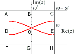
Figure 1: The Weierstrass function fundamental domain on complex plane.

Let us examine limit cases.

In the limit case of free electrons the gap in the spectrum vanishes. Let us put $\varepsilon_{2}=\varepsilon_{3}=-\left({{\eta}^{\prime}/{\omega}^{\prime}}\right)$ then $\varepsilon_{1}=2\left({{\eta}^{\prime}/{\omega}^{\prime}}\right)$ and

$$k=\int\limits_{\varepsilon_{1}}^{E}{\frac{dz}{{2\sqrt{\left({z-\varepsilon_{1}}\right)}}}}=\sqrt{\left({E-\varepsilon_{1}}\right)},$$

or $E=\varepsilon_{1}+k^{2}$.

In the limit case of a very wide gap, we pass to another variable $z=\left({1/2}\right)\cdot\left({\varepsilon_{1}+\varepsilon_{2}}\right)+\left({1/2}\right)\cdot\left({\varepsilon_{2}-\varepsilon_{1}}\right)\varphi$ in the integral (25). Using expression $e_{1}+e_{2}+e_{3}=0$ and introducing the designation $A=(2E-\varepsilon_{1}-\varepsilon_{2})/(\varepsilon_{2}-\varepsilon_{1}),\>\>A\in[-1;1]$ we derive the following

$$k=\int\limits_{-1}^{A}\frac{{\frac{1}{2}\left({\varepsilon_{1}+\varepsilon_{2}}\right)+{{\eta}^{\prime}/{\omega}^{\prime}}+\frac{1}{2}\left({\varepsilon_{2}-\varepsilon_{1}}\right)\varphi}}{{2\sqrt{(1-\varphi^{2})(\frac{3}{2}\varepsilon_{3}-\frac{1}{2}\left({\varepsilon_{2}-\varepsilon_{1}}\right)\varphi)}}}d\varphi.$$

Expanding the expression under the integral to the order of $\varepsilon_{2}-\varepsilon_{1}$ and restricting ourselves to the zero approximation, we obtain the spectrum in the limit case of tight binding electrons.

$$E=\frac{1}{2}\left({\varepsilon_{1}+\varepsilon_{2}}\right)-\frac{1}{2}\left({\varepsilon_{2}-\varepsilon_{1}}\right)\cos\left({ka}\right),$$

where

$$a=\frac{2\sqrt{\frac{3}{2}\varepsilon_{3}}}{\frac{1}{2}(\varepsilon_{1}+\varepsilon_{2})+\frac{\eta^{\prime}}{\omega^{\prime}}}\>.$$

It is possible to determine effective masses at band edges. According to the expression (25), we have

$$k= \int\limits_{\varepsilon_{1}}^{E}\left(\frac{{\varepsilon_{1}+\left({{\eta}^{\prime}/{\omega}^{\prime}}\right)}}{{\sqrt{\left({\varepsilon_{2}-\varepsilon_{1}}\right)\left({\varepsilon_{3}-\varepsilon_{1}}\right)}}}\cdot\frac{1}{2\sqrt{z-\varepsilon_{1}}}\right.$$

$$+\left.O\left((z-\varepsilon_{1})^{1/2}\right)\right)dz,$$

that leads to following expansions,

$$E=\varepsilon_{1}+\frac{k^{2}}{m_{1}^{*}}+O(k^{3});\;\;\;\;\frac{1}{m^{*}_{1}}=\frac{2(\varepsilon_{2}-\varepsilon_{1})(\varepsilon_{3}-\varepsilon_{1})}{(\varepsilon_{1}+{\eta}^{\prime}/{\omega}^{\prime})^{2}},$$ (26)

$$E=\varepsilon_{2}+\frac{k^{2}}{m_{2}^{*}}+O(k^{3});\;\;\;\;\frac{1}{m^{*}_{2}}=-\frac{2(\varepsilon_{2}-\varepsilon_{1})(\varepsilon_{3}-\varepsilon_{2})}{(\varepsilon_{2}+{\eta}^{\prime}/{\omega}^{\prime})^{2}}.$$ (27)

Here we denote by $m_{1}^{*}$ and $m_{2}^{*}$ respectively the effective masses at the bottom edge and at the top edge of the first band. The effective mass $m_{1}^{*}$ is positive and $m_{2}^{*}$ is negative. One can see that the both effective masses depend on all the band edges.

II.2 The two-gap Lame potential ($\ell=2$)

For the two-gap Lame potential the band edges are the following,

$$\varepsilon_{1}=-\sqrt{3g_{2}},\;\;\varepsilon_{2}=-3 e_{1},\;\;\varepsilon_{3}=-3e_{2},$$

$$\varepsilon_{4}=-3e_{3},\;\;\varepsilon_{5}=\sqrt{3g_{2}}.$$ (28)

The expression $\Lambda(x,E)$ in this case is presented in such a way,

$$\Lambda(x,E)=18\wp^{2}(ix+\omega)-6E\wp(ix+\omega)+2E^{2}-\frac{9}{2}g_{2}$$

$$=18[\wp(ix+\omega)-\wp(t_{1})]\>[\wp(ix+\omega)-\wp(t_{2})]$$

$$=2\left[\frac{3}{2}\left(\wp(ix+\omega)-\sqrt{g_{2}-3\wp^{2}(ix+\omega)}\right)-E\right]$$

$$\times\left[\frac{3}{2}\left(\wp(ix+\omega)+\sqrt{g_{2}-3\wp^{2}(ix+\omega)}\right)-E\right].$$ (29)

The spectrum of the Schrödinger equation (3) with the two-gap Lame potential in parametric form is the following

$$\left\{\begin{array}[c]{rcl}k&=&\left(\zeta(t_{1})-\frac{\eta^{\prime}}{\omega^{\prime}}t_{1}\right)+\left(\zeta(t_{2})-\frac{\eta^{\prime}}{\omega^{\prime}}t_{2}\right),\\ \wp(t_{1})&=&\frac{E}{6}+\frac{1}{2\sqrt{3}}\sqrt{3g_{2}-E^{2}},\\ \wp(t_{2})&=&\frac{E}{6}-\frac{1}{2\sqrt{3}}\sqrt{3g_{2}-E^{2}}.\par\end{array}\right.$$ (30)

The expression for dependence $k$ on $E$ can be written in the form of hyperelliptic integral

$$k=k_{o}+\int\limits_{E_{0}}^{E}\frac{\frac{3\sqrt{2}\eta^{\prime}}{\omega^{\prime}}z+\frac{1}{\sqrt{2}}\left(2z\>^{2}-3g_{2}\right)}{\sqrt{\left(z^{2}-3g_{2}\right)\left(8z\>^{3}-18g_{2}z+54g_{3}\right)}}dz,$$ (31)

When $E$ takes on values in the first band the parameters $t_{1}$ and $t_{2}$ take on values in the line $AC$ (Fig. 1). When $E$ takes on values in the second band the parameter $t_{1}$ takes on values in the line $AC$ and the parameter $t_{2}$ takes on values in the line $DE$. In both cases $\wp(t_{1})$ and $\wp(t_{2})$ are real. The situation changes when $E$ takes on values in the third band. In this case $\wp(t_{1})$ and $\wp(t_{2})$ are complex conjugate ($k$ and $E$ remain real), $t_{1}$ and $t_{2}$ take on values in the curves which are depicted inside fundamental domain $ACHF$ (while constructing, we used $\omega=1,\>\omega^{\prime}=i$).

With the help of the Hermite reduction, we can express the integral (31) through the standard elliptic integrals of the first and the second kinds BE1 ; BE2 and represent the spectrum in other parametric form. Let us put

$$y=\frac{2z\>^{3}-b}{3(z\>^{2}-a)},\;\>a=3g_{2},\;\>b=-54g_{3}.$$

Using equalities

$$\int\limits_{E_{0}}^{E}\frac{zdz}{\sqrt{\left(z^{2}-a\right)\left(8z\>^{3}-6az-b\right)}}=\frac{1}{2\sqrt{3}}\int\limits_{Y_{0}}^{Y}\frac{dy}{\sqrt{y^{3}-3ay+b}},$$

$$\left.\int\limits_{E_{0}}^{E}\frac{(2z^{2}-a)dz}{\sqrt{\left(z^{2}-a\right)\left(8z\>^{3}-6az-b\right)}}-\left[\frac{1}{3}\sqrt{\frac{8z^{3}-6az-b}{z^{2}-a}}\right]\right|^{E}_{E_{0}}$$

$$=\frac{1}{2\sqrt{3}}\int\limits_{Y_{0}}^{Y}\frac{ydy}{\sqrt{y^{3}-3ay+b}},$$

and putting $y=6\wp(h)$, we can write the integral (31) in terms of elliptic functions

$$\left\{\begin{array}[c]{rcl}\wp(h)&=&\frac{E^{3}+27g_{3}}{9E^{2}-27g_{2}}\;,\\ k&=&\zeta(h)-\frac{\eta^{\prime}}{\omega^{\prime}}h-\frac{2}{3}\sqrt{\frac{(E+3e_{1})(E+3e_{2})(E+3e_{3})}{E^{2}-3g_{2}}}\;.\end{array}\right.$$ (32)

In this form the spectrum of the two-gap potential is provided in the paper. P

By the same way as in the case of one-gap potential we derive expressions for effective masses in the first band,

$$E=\varepsilon_{1}+\frac{k^{2}}{m_{1}^{*}}+O(k^{3}),$$

$$\frac{1}{m^{*}_{1}}=\frac{2(\varepsilon_{2}-\varepsilon_{1})(\varepsilon_{3}-\varepsilon_{1})(\varepsilon_{4}-\varepsilon_{1})(\varepsilon_{5}-\varepsilon_{1})}{\left((\varepsilon_{1})^{2}+3({\eta}^{\prime}/{\omega}^{\prime})\varepsilon_{1}-\frac{3}{2}g_{2}\right)^{2}},$$ (33)

$$E=\varepsilon_{2}+\frac{k^{2}}{m_{2}^{*}}+O(k^{3}),$$

$$\frac{1}{m^{*}_{2}}=-\frac{2(\varepsilon_{2}-\varepsilon_{1})(\varepsilon_{3}-\varepsilon_{2})(\varepsilon_{4}-\varepsilon_{2})(\varepsilon_{5}-\varepsilon_{2})}{\left((\varepsilon_{2})^{2}+3({\eta}^{\prime}/{\omega}^{\prime})\varepsilon_{2}-\frac{3}{2}g_{2}\right)^{2}},$$ (34)

where $m_{1}^{*}$ and $m_{2}^{*}$ are effective masses at the bottom and at the top band edges respectively. One can see that the effective masses depend on all the band edges, the same as in an one-gap case. In Table 1, the effective mass values are provided for different values of the parameter $|\tau|$, we put a period of the potential $T=|2\omega^{\prime}|=2$.

Table 1: Inverse effective masses for the first band in case of the two-gap Lame potential.

$\tau$	$1/m^{*}_{1}$	$1/m^{*}_{2}$
0.55	1.99	-47.34
0.74	1.89	-10.03
1	1.25	-2.13
1.23	0.57	-0.67
1.52	0.15	-0.16
2.18	0.005	-0.005

In Table 1, one can see that with the increase of the value of $|\tau|$, the values of $|1/m^{*}_{1}|$ and $|1/m^{*}_{2}|$ decrease. When the band degenerates into an energy level that corresponds to the limit case of tight binding electrons, $m^{*}_{1}\rightarrow\infty,\;m^{*}_{2}\rightarrow-\infty$. We obtain so called ”heavy” electrons. In the other limit case of free electrons, $m^{*}_{1}$ tends to the mass of free electron, i.e. $m^{*}_{1}\rightarrow 1/2$. And since the gap width vanishes, $m^{*}_{2}\rightarrow-0$ in this case.

In Fig 2, we provide the graphs $E=E(k)$ and $U(x)$ for the two-gap potential corresponding to different values of the parameter $\left|\tau\right|=\left|{\omega^{\prime}}\>/{\omega}\right|$. As $|\tau|$ increases, the width of the gaps increase. There are the limit cases of very narrow gaps and very wide gaps in this figure. With increase of $|\tau|$, the second band also degenerates into an energy level.

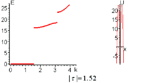
Figure 2: Dispersion relation $E=E(k)$ and potential $U(x)$ in case of the two-gap Lame potential for different values of the parameter $\left|\tau\right|=\left|{\omega^{\prime}}\>/{\omega}\right|$.

III The separable finite-gap Lame potential

The one-electron separable Hamiltonian has the form

$$H=\sum\limits_{j=1}^{n}H_{j}=\sum\limits_{j=1}^{n}\left(-\frac{\partial^{2}}{\partial x_{j}^{2}}+U_{j}(x_{j})\right).$$ (35)

In general case $n\in\mathbb{N},$ but we consider below only the three dimensional case, $n=3.$ We will use the finite-gap Lame potentials for the potentials $U_{j}(x_{j})$. In general case of the orthorhombic lattice every one-dimensional potential $U_{j}(x_{j})$ is characterized by its own parameters $\omega,\>\omega^{\prime}$,

$$H=-\partial_{x}^{2}-\partial_{y}^{2}-\partial_{z}^{2}-\ell_{x}(\ell_{x}+1)\wp(ix+\omega_{x})$$

$$-\ell_{y}(\ell_{y}+1)\wp(iy+\omega_{y})-\ell_{z}(\ell_{z}+1)\wp(iz+\omega_{z}).$$ (36)

In Fig. 3, the three dimensional one-gap potential for $z=0$ is represented with the following half-periods: $\omega_{x}=\omega_{y}=1,\;\omega^{\prime}_{x}=\omega^{\prime}_{y}=i$.

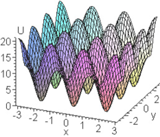
Figure 3: The three dimensional one-gap Lame potential for fixed value of the variable $z$, we put $z=0$, $\omega_{x}=\omega_{y}=1,\;\omega^{\prime}_{x}=\omega^{\prime}_{y}=i$.

An eigenfunction of the Hamiltonian (36) is a product of one-dimensional eigenfunctions of every $H_{j}$,

$$\Psi_{\mathbf{I},\;\mathbf{k}}(\mathbf{x})=\prod\limits_{j=1}^{3}\Psi_{I_{j},\;k_{j}}(x_{j}),$$ (37)

where $\textbf{I}=(I_{1},I_{2},I_{3}),\;$ $I_{j}\in\{1,..,\ell_{j}\}$ is a band number. The expression for energy consists of three terms,

$$E_{\mathbf{I}}(\mathbf{k})=E_{I_{1}}(k_{1})+E_{I_{2}}(k_{2})+E_{I_{3}}(k_{3}).$$ (38)

The Fermi surface is described by the following equation

$$E_{F}=E_{\mathbf{I}}(\mathbf{k}+\mathbf{b}),$$

were $E_{F}$ is the Fermi energy. Here the wavevector $\mathbf{k}$ takes on values in the Brillouin zone, every solution of this equation for a prescribed value of dual lattice vector $\mathbf{b}$ defines one of sheets of the Fermi surface. The set of dual lattice vectors corresponds to their set in Fourier series expansion of a separable potential. If the real electron potential differs a bit from the separable one, then the corresponding corrections can be taken into account using the perturbation theory.

Let us examine the limit case of very narrow gaps. Since the potential periods $T_{j}=2|\omega_{j}^{\prime}|$ are fixed, let $\omega_{j}\rightarrow\infty$. Then, potentials $U_{j}(x)$ tend to constants, the dependence of energy on wavevector becomes quadratic and the Fermi surface sheets are similar to pieces of spherical surface. Thus, our model is the considerable generalization of the Harrison method that was successfully used to construct the Fermi surfaces of metals. H

Let us examine the other limit case of very wide gaps. Since we fixed the potential periods $T_{j}=2|\omega_{j}^{\prime}|$, let $\omega_{j}\rightarrow 0$. Then, $e_{2}^{(j)}-e_{3}^{(j)}\rightarrow 0$. It is obvious that in this case all the bands degenerate into levels. The finite-gap spectrum of tight binding electrons is similar to the spectrum that is obtained in the well-known LCAO method. In this case function $\Psi_{I_{0},\;0}\left({x}\right);\>{I_{0}=\left({0,0,0}\right)}$ corresponds to $s$-state. The three functions $\Psi_{I_{1},\;0}\left({x}\right),$ $\Psi_{I_{2},\;0}\left({x}\right),$ $\Psi_{I_{3},\;0}\left({x}\right);$ $I_{1}=({1,0,0}),$ $I_{2}=({0,1,0}),$ $I_{3}=\left({0,0,1}\right)$ correspond to $p$-state as they are proportional to $x$, $y$, $z$ respectively when the space variables tend to zero. The six functions $\Psi_{I_{4},\;0}({x})$, $\Psi_{I_{5},\;0}({x})$, $\Psi_{I_{6},\;0}({x})$, $\Psi_{I_{7},\;0}({x})$, $\Psi_{I_{8},\;0}({x})$, $\Psi_{I_{9},\;0}({x})\>$; $I_{4}=\left({1,1,0}\right)$, $I_{5}=\left({1,0,1}\right)$, $I_{6}=\left({0,1,1}\right)$, $I_{7}=\left({2,0,0}\right)$, $I_{8}=\left({0,2,0}\right)$, $I_{9}=\left({0,0,2}\right)$ split into five functions that correspond to $d$-state and one function corresponds to the $s$-state since these functions are proportional to $xy,\;xz,\;yz$, $x^{2}-a,\;y^{2}-b,\;z^{2}-c$ respectively when the space variables tend to zero. BBK2

The Fermi surfaces for cubic lattice are represented in Fig. 3-5. They are constructed using the separable one-gap Lame potential for different values of the parameter $|\tau|$. In Fig. 3, the Fermi surfaces in the first band are represented at $E_{F}=2.43$. The Fermi surface sheets don’t appear in the second band at this value of $E_{F}$. In Fig. 4, the open Fermi surfaces are represented at $E_{F}=3.8$ in the first band. In Fig. 5, the closed Fermi surfaces are represented at the same value of $E_{F}$ in the second band.

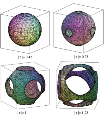
Figure 4: The Fermi surface in the first band for different values of the parameter $\left|\tau\right|=\left|{\omega^{\prime}}\>/{\omega}\right|$, the Fermi energy is $E_{F}=2.43$.

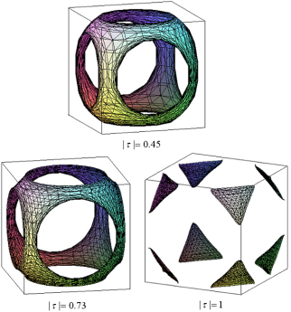
Figure 5: The Fermi surface in the first band for different values of the parameter $\left|\tau\right|=\left|{\omega^{\prime}}\>/{\omega}\right|$, the Fermi energy is $E_{F}=3.8$.

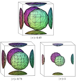
Figure 6: The Fermi surface in the second band for different values of the parameter $\left|\tau\right|=\left|{\omega^{\prime}}\>/{\omega}\right|$, the Fermi energy is $E_{F}=3.8$.

IV The Lifshits singularities of the electron thermodynamic potential and the one-gap Lame potential

It is known that the density of states in a crystal

$$\nu(E)=\frac{dN(E)}{dE}=\frac{2V}{(2\pi)^{3}}\int\limits_{E(\mathbf{k})=E}\frac{dS}{|\mathbf{\nabla}E(\mathbf{k})|},$$

as a function of the variable $E$ has singularities which are named the Van Hove ones.V They occur when the electron group velocity vanishes, $\mathbf{\nabla}E(\mathbf{k_{c}})=0$. Since $E(\mathbf{k})$ is a smooth function of the wavevector $\mathbf{k}$, it can be expanded into the Taylor series about a critical wavevector $\mathbf{k_{c}}.$ Restricting ourselves to quadratic terms, we obtain

$$E=E_{c}+\alpha_{1}\xi_{1}^{2}+\alpha_{2}\xi_{2}^{2}+\alpha_{3}\xi_{3}^{2}+O(\xi^{3}),$$

where $\mathbf{\xi}=\mathbf{k}-\mathbf{k_{c}}$. Depending on signs of the coefficients ${\alpha_{1},\alpha_{2},\alpha_{3}}$ the four types of critical points are distinguished, they are a minimum value, a maximum value and two types of saddle points. In a three dimensional crystal the function $\nu(E)$ at the critical energy $E_{c}$ is continuous but its derivative at this point has infinite discontinuity.

The function $E(\mathbf{k})$ is periodic with respect to every component of the wavevector $\mathbf{k}=(k_{x},k_{y},k_{z}),$ it means the energy $E(k_{x},k_{y},k_{z})$ is defined on three dimensional torus. This function has a denumerable set of branches and every one of them corresponds to a certain energy band. The function $E(k_{x},k_{y},k_{z})$ is differentiable and regular so, according to elementary facts of topology, for each of the branches the number of critical points relates to the Betti numbers of the manifold, where the function $E$ is being defined. Thus, every branch of the function $E(k_{x},k_{y},k_{z})$ has one maximum value, one minimum value and three saddle points of every type. But in a real crystal the bands may overlap and as a result the singularities of the function $\nu(E)$, that are related to different branches, may compensate each other.

In 1952 Van Hove examined singularities of the elastic frequency distribution of a crystal (that are similar to singularities of the electron density of states) and showed that for a three dimensional crystal the frequency distribution function has at least one saddle point of every types and its derivative takes on the value $-\infty$ at the upper end of the spectrum. V

In 1960 I.M. Lifshits connected singularities of the density of electron states with a variation of the Fermi surface topology. L He showed that at zero temperature the electron phase transitions occur at the special energies, they were later named the Lifshits electron phase transitions of $2\frac{1}{2}$ kind. Singularities of the conduction electron spectrum at the point of such a transition lead to anomalies of thermodynamic and kinetic quantities. When temperature increases, this transition smoothes out.

At present, the Van Hove singularities are considered as one of the reasons for the origin of high-temperature superconductivity. M

Let us consider the Schrödinger equation with the one-gap separable Lame potential that corresponds to the tetragonal Bravais lattice,

$$-\mathbf{\Delta} \Psi+W(x,y,z)\Psi=E\Psi,$$

$$W(x,y,z)= -2\wp(ix+\tilde{\omega}|\tilde{\omega},\tilde{\omega}^{\prime}\>)$$

$$-2\wp(iy+\tilde{\omega} |\tilde{\omega},\tilde{\omega}^{\prime}\>)-2\wp(iz+\omega|\omega,\omega^{\prime}\>)-e_{3}+4\tilde{e}_{1}.$$

In order to describe the Lifshits electron transformation, it is enough to examine the case when the Fermi surface is open only at two opposite sides of the Brillouin zone. Let us choose half periods and the Fermi energy so that the Fermi surface has the form of a goffered cylinder which is prolate along the direction $k_{z}$, as in Fig. 7. In this case we have to put $\tilde{\omega}>\omega,\>|\tilde{\omega}^{\prime}\>|>|\omega^{\prime}\>|$ (while constructing, we used $\tilde{\omega}=1,\;\tilde{\omega}^{\prime}=0.65i;\;\omega=0.3,\;\omega^{\prime}=0.5i$). Then, in order to simplify computations, we can expand potential with respect to the variables $x,\>y$ and restrict ourselves to zero approximation.

Figure 7: The Fermi surface in the first band in the form of a goffered cylinder, we put $\tilde{\omega}=1,\;\tilde{\omega}^{\prime}=0.65i;\;\omega=0.3,\;\omega^{\prime}=0.5i$.

The spectrum of the Schrödinger operator with the potential

$$U(x,y,z)=-e_{3}-2\wp(iz+\omega|\omega,\omega^{\prime}\>)$$ (39)

looks as follows:

$$\left\{\begin{array}[c]{rcl}E(k_{x},k_{y},h_{z})&=&k_{x}^{2}+k_{y}^{2}-e_{3}+\wp\left(h_{z}\right),\\ k_{z}(h_{z})&=&\zeta(h_{z})-\frac{\eta^{\prime}}{\omega^{\prime}}\;h_{z}\;.\end{array}\right.$$ (40)

The function $E(k_{x},k_{y},k_{z})$ has two critical points in the first band that are a minimum value and a saddle point and one critical point in the second band that is a minimum value. We will consider below only the first band.

One can see that $E|_{\mathbf{k}=0}=0$. Let us put $K^{2}=k_{x}^{2}+k_{y}^{2}$. For the first band $h_{z}=t+\omega^{\prime},\>t\in[-\omega;\>\omega]$. Since, the function $E(\mathbf{k})$ is even, it is enough to consider the case when $t\in[0;\>\omega]$. The expression for the number of states is the following

$$N(E)=\frac{2V}{(2\pi)^{3}}\int dk_{x}dk_{y}dk_{z}=\frac{2V}{(2\pi)^{3}}\int{\pi K^{2}dk_{z}}$$

$$=\frac{2V}{(2\pi)^{3}}\int{\pi\left(E+e_{3}-\wp\left(h_{z}\right)\right)dk_{z}}$$

$$=\frac{2V}{(2\pi)^{3}}\int{\pi\left(E+e_{3}-\wp\left(h_{z}\right)\right)\left(-\wp\left(h_{z}\right)-\frac{\eta^{\prime}}{\omega^{\prime}}\right)dh_{z}},$$ (41)

where $V$ is dimensionless volume.

It easy to show that at the energy $E_{c}=-e_{3}+e_{2}$ the Fermi surface opens on the boundary of the Brillouin zone which is orthogonal to the axis $k_{z}.$ In this case we can express the number of states (41) in such a form,

$$N(E)=\frac{V}{2\pi^{2}}\int\limits_{0}^{t_{0}}{\left(E+e_{3}-\wp\left(t+\omega^{\prime}\>\right)\right)\left(-\wp\left(t+\omega^{\prime}\>\right)-\frac{\eta^{\prime}}{\omega^{\prime}}\right)dt}$$ (42)

$$=\frac{V}{2\pi^{2}}\left[\left(\frac{g_{2}}{12}-\frac{\eta^{\prime}}{\omega^{\prime}}(E+e_{3})\right)t_{0}+\left(\zeta(t_{0}+\omega^{\prime}\>)-\eta^{\prime}\>\right)\left((E+e_{3})-\frac{\eta^{\prime}}{\omega^{\prime}}\right)+\frac{1}{6}\wp^{\prime}\left(t_{0}+\omega^{\prime}\>\right)\right].$$ (43)

Here we have introduced the parameter $t_{0}$ as follows.

A. Under condition $0\leq E<E_{c}$ we define the parameter $t_{0}$ by the equality

$$E+e_{3}=\wp\left(t_{0}+\omega^{\prime}\right).$$

According to this equality, the function $t_{0}=t_{0}(E)$ is differentiable and has a derivative

$$\frac{dt_{0}}{dE}=\frac{1}{\wp^{\prime}\left(t_{0}+\omega^{\prime}\right)}.$$

B. Under condition $E>E_{c}$ we define the parameter $t_{0}$ by the equality $t_{0}=\omega$.

Differentiating this expression for the number of states in $E$ and using the definition of parameter $t_{0}$ we obtain the electron density of states,

$$\nu(E) =\frac{dN(E)}{dE}=\frac{V}{2\pi^{2}}\int\limits_{0}^{t_{0}}{\left(-\wp\left(t+\omega^{\prime}\>\right)-\frac{\eta^{\prime}}{\omega^{\prime}}\right)dt}$$ (44)

$$=\frac{V}{2\pi^{2}}\left(\zeta(t_{0}+\omega^{\prime}\>)-\frac{\eta^{\prime}}{\omega^{\prime}}\>(t_{0}+\omega^{\prime}\;)\right)$$ (45)

$$=\left\{\begin{array}[c]{rcl}\frac{V}{2\pi^{2}}|\mathbf{k}(E)|,&&E<E_{c}\\ \frac{V}{2\pi}\cdot\frac{1}{2|\omega^{\prime}|},&&E>E_{c}\end{array}\right..$$ (48)

Even though this expression was derived for the one-gap potential, it is correct in a case of any $\ell-$gap potential.

Let us expand the function $\nu(E)$ under the condition $E<E_{c}$ in the $\sqrt{E}$ powers. We derive the following formula,

$$\nu(E)=\frac{V\;E^{1/2}}{2\pi^{2}C^{1/2}}+O(E^{3/2}),\quad C=\frac{6e_{3}^{2}-\frac{g_{2}}{2}}{2(e_{3}+\frac{\eta^{\prime}}{\omega^{\prime}})^{2}}.$$ (49)

It is obvious that the first term in the expansion (49) corresponds to the function $E(k_{x},k_{y},k_{z})=k_{x}^{2}+k_{y}^{2}+C_{z}k_{z}^{2}$.

Let us calculate the first derivative of the density of states. We should distinguish two cases.

A. Under condition $0\leq E<E_{c}$ we obtain the expression

$$\frac{d\nu(E)}{dE}=-\frac{V}{2\pi^{2}}\cdot\frac{\wp\left(t_{0}+\omega^{\prime}\>\right)+\frac{\eta^{\prime}}{\omega^{\prime}}}{\wp^{\prime}\left(t_{0}+\omega^{\prime}\>\right)}$$

$$=-\frac{V}{4\pi^{2}}\cdot\frac{\frac{\eta^{\prime}}{\omega^{\prime}}+e_{3}+E}{E^{1/2}(e_{1}-e_{3}-E)^{1/2}}\cdot\frac{1}{(E_{c}-E)^{1/2}}.$$ (50)

B. Under condition $E>E_{c}$ we obtain the expression

$$\frac{d\nu(E)}{dE}=0.$$ (51)

The singularity at the point $E=e_{1}-e_{3}$ corresponds to the Fermi surface appearance in the second band. The singularity at the point $E=0$ corresponds to the minimum value of $E$ in the first band (the Fermi surface appears in the center of the Brillouin zone). The singularity at the point $E=E_{c}$ corresponds to the saddle point (the Fermi surface opens on the boundary of the Brillouin zone). In all three cases the singularities have positive signs. We will consider further only the case $E=E_{c}$, it is obvious that the other two cases can be considered similarly.

Let us introduce the following notation:

$$\frac{\alpha}{2}=-\frac{V}{4\pi^{2}}\cdot\frac{\frac{\eta^{\prime}}{\omega^{\prime}}+e_{2}}{(e_{2}-e_{3})^{1/2}(e_{1}-e_{2})^{1/2}}$$

$$=\frac{V}{4\pi^{2}}\cdot\frac{|\frac{\eta^{\prime}}{\omega^{\prime}}+e_{2}|}{(e_{2}-e_{3})^{1/2}(e_{1}-e_{2})^{1/2}},$$

$$A=\frac{V}{2\pi^{2}}\cdot\left(\frac{g_{2}}{12}\omega+\frac{\pi}{2|\omega^{\prime}\>|}e_{3}-\frac{\eta\eta^{\prime}}{\omega^{\prime}}\>\right),$$

$$B=\frac{V}{2\pi}\cdot\frac{1}{2|\omega^{\prime}\;|},$$

$$C=-\frac{V}{2\pi^{2}}\left[\frac{e_{2}^{2}}{2}\cdot\frac{\pi}{2|\omega^{\prime}|}+e_{2}\left(\frac{g_{2}}{12}\omega-\frac{\eta^{\prime}}{\omega^{\prime}}\eta\right)+\frac{3}{40}g_{2}\eta\right.$$

$$\left.-\omega\left(\frac{\eta^{\prime}}{\omega^{\prime}}\cdot\frac{g_{2}}{12}+\frac{1}{20}g_{3}\right)\right].$$

In order to compute the thermodynamics potential $\Omega(T,V,\mu)$ we expand the following expressions $d\nu(E)/dE,\>$ $\nu(E),\>$ $N(E)$ in the $(E_{c}-E)^{1/2}$ powers. We derive the following expressions:

$$\frac{d\nu(E)}{dE}=\left\{\begin{array}[]{lr}\frac{\alpha}{2}\cdot\frac{1}{(E_{c}-E)^{1/2}}\\ \hskip 34.14322pt+O\left((E_{c}-E)^{1/2}\right),&E<E_{c},\\ 0,&E>E_{c},\end{array}\right.$$ (52)

$$\nu(E)=\left\{\begin{array}[]{lr}B-\alpha(E_{c}-E)^{1/2}\\ \hskip 42.67912pt+O\left((E_{c}-E)^{3/2}\right),&E<E_{c},\\ B,&E>E_{c},\end{array}\right.$$ (53)

$$N(E)=\left\{\begin{array}[]{lr}A+BE+\frac{2}{3}\alpha(E_{c}-E)^{3/2}\\ \hskip 36.98866pt+O\left((E_{c}-E)^{5/2}\right),&E<E_{c},\\ A+BE,&E>E_{c}.\end{array}\right.$$ (54)

The coefficient $\alpha$ is expressed in terms of the effective mass $m_{2}^{*}$ along the $k_{z}$ direction at the top edge of the first band,

$$\alpha=\frac{V}{\sqrt{2}\pi^{2}}\sqrt{-m_{2}^{*}}\;.$$ (55)

Hence the coefficient $\alpha$ depends on all the band edges and $\alpha\in[0;\infty)$. When the gap width decreases on boundary of the Brillouin zone, which is orthogonal to the $k_{z}$ axis, the value of the coefficient $\alpha$ decreases also. In the limit case of extremely wide gap the parameter $\alpha\rightarrow\infty$. In this case the problem from a three-dimensional one becomes two-dimensional and we should use other speculations. In the other limit case when the gap width vanishes the parameter $\alpha\rightarrow 0$. It is obvious: when the gap width equals zero the value $E_{c}$ is not a critical point.

Thermodynamic potential at a normal metal is defined by the following expression

$$\Omega(T,V,\mu) =-\int\limits_{0}^{\infty}\frac{N(\varepsilon)d\varepsilon}{1+exp\left(\frac{\varepsilon-\mu}{T}\right)},$$ (56)

$$\Omega(0,V,\mu) =\Omega_{0}=-\int\limits_{0}^{\mu}N(\varepsilon)d\varepsilon\;.$$ (57)

Using the expression (43) we can calculate the integral (57) and find the analytical expression for $\Omega(0,V,\mu)$, but this expression will be quite a complicated one and we do not adduce it.

Using the formula (54) we present the electron thermodynamic potential $\Omega_{0}$ in a neighborhood of the critical value of energy in such a form,

$$\Omega_{0}=\left\{\begin{array}[c]{lcl}C+AE_{c}+\frac{1}{2}BE_{c}^{2}-A\mu-\frac{1}{2}B\mu^{2}+\frac{4}{15}\alpha(E_{c}-\mu)^{5/2}+O\left((E_{c}-\mu)^{7/2}\right),&&\mu<E_{c},\\ C+AE_{c}+\frac{1}{2}BE_{c}^{2}-A\mu-\frac{1}{2}B\mu^{2},&&\mu>E_{c}.\end{array}\right.$$ (58)

The variation $\delta N(E)$ of number of states looks as follows:

$$\delta N(E)=\left\{\begin{array}[c]{lcl}\frac{2}{3}\alpha(E_{c}-E)^{3/2},&&E<E_{c},\\ 0,&&E>E_{c}.\end{array}\right.$$

Then the variation of the electron thermodynamic potential can be written down in such a way

$$\delta\Omega(T,V,\mu)=-\int\limits_{0}^{\infty}\frac{\delta N(\varepsilon)d\varepsilon}{1+exp\left(\frac{\varepsilon-\mu}{T}\right)}\;.$$

We provide below the asymptotic expansion of the expression $\delta\Omega(T,V,\mu)$ under condition $T\rightarrow 0,$

$$\delta\Omega=\left\{\begin{array}[]{lr}-\frac{4}{15}\alpha E_{c}^{5/2}+\frac{4}{15}\alpha(E_{c}-\mu)^{5/2}+\frac{\alpha}{6}\pi^{2}T^{2}(E_{c}-\mu)^{1/2}+O(T^{4}),&\mu<E_{c},\\ -\frac{4}{15}\alpha E_{c}^{5/2}+\frac{\sqrt{\pi}}{2}\alpha T^{5/2}\exp\left(\frac{-|E_{c}-\mu|}{T}\right)erf\left(\sqrt{\frac{E_{c}}{T}}\right)+O\left(\left(\exp\left(\frac{-|E_{c}-\mu|}{T}\right)\right)^{2}\right),&\mu>E_{c}.\end{array}\right.$$ (59)

A similar expression was presented in the paper. L

In Fig. 8, the graph $\partial_{\mu}^{3}\Omega(T,V,\mu)$ on the temperature $T$ and the chemical potential $\mu$ is represented (while constructing, we used $V=20$, $\omega=0.3,\;\omega^{\prime}=0.5i$, accordingly $E_{c}=2.5$). One can see that when $\mu\rightarrow E_{c},\>T=0$ the third derivative from the thermodynamics potential has an infinite discontinuity and

$$\lim\limits_{\mu\rightarrow E_{c}+0}\partial_{\mu}^{3}\Omega(0,V,\mu)=0,\;\lim\limits_{\mu\rightarrow E_{c}-0}\partial_{\mu}^{3}\Omega(0,V,\mu)=-\infty\;.$$

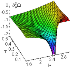
Figure 8: Third derivative of thermodynamics potential, we put $V=20$, $\omega=0.3,\;\omega\acute{}=0.5i$ and $E_{c}=2.5$. Thermodynamics potential, temperature and chemical potential take on dimensionless values. $\partial_{\mu}^{3}\Omega(T,V,\mu)$ has an infinite discontinuity when $\mu\rightarrow E_{c},\>T=0$.

One can see also that the singularity at the point $\mu=E_{c}$ smoothes out with the temperature increase. In order to estimate an appropriate temperature interval, we should pass from dimensionless units to Kelvin degrees. In order to do this we have to multiply the dimensionless temperature by the following coefficient,

$$\frac{E_{0}}{k_{b}}=\frac{\hbar^{2}}{2ma^{2}k_{b}}=\frac{\hbar^{2}}{2m\left(c/2|\omega^{\prime}\>|\right)^{2}k_{b}},$$ (60)

where $k_{b}$ is the Boltzmann constant and $c$ is a period of crystal potential. If the potential period equals $3\AA$ and effective electron mass is put $10m_{e}$, where $m_{e}$ - mass of free electron, we find out that the dimensionless temperature value $0.1$ corresponds to the temperature value in standard units $\sim 49^{0}K$. Since the width of the area $\bigtriangleup(E_{c}-\mu),$ which contributes to the singularity of $\partial_{\mu}^{3}\Omega(T,V,\mu),$ is proportional $T$, then in a general case the singularity smoothes out slowly enough with the temperature increase.

V Magnetization singularities of the Pauli paramagnetics

A magnetization of an electron gas in magnetic field is described by the following expression,

$$M(T,\mu,H) =\frac{\beta}{2}\int\limits_{0}^{\infty}\left(\frac{1}{1+exp\left(\frac{\varepsilon-\mu-\beta H}{T}\right)}\right.$$

$$\left.-\frac{1}{1+exp\left(\frac{\varepsilon-\mu+\beta H}{T}\right)}\right)\nu(\varepsilon)d\varepsilon,$$ (61)

where $\beta={e\hbar}/{2mc}$ is the Bohr magneton, $H$ is an external magnetic field, $T$ is a temperature. According to this expression the magnetization at $T=0$ can be presented in the following way,

$$M(0,\mu,H)=M_{0}=\frac{\beta}{2}\left(N(\mu+\beta H)-N(\mu-\beta H)\right).$$ (62)

Let us expand the expression (62) in the $(E_{c}-\mu\pm\beta H)^{1/2}$ powers. Using the formula (54) we come to the following result,

$$M_{0}=\left\{\begin{array}[c]{lcl}\frac{\beta}{2}(2\beta HB+\frac{2}{3}\alpha(E_{c}-\mu-\beta H)^{3/2}-\frac{2}{3}\alpha(E_{c}-\mu+\beta H)^{3/2}\\ \hskip 170.71652pt+O((E_{c}-\mu\pm\beta H)^{5/2})),&&\mu<E_{c}-\beta H,\\ \frac{\beta}{2}(2\beta HB-\frac{2}{3}\alpha(E_{c}-\mu+\beta H)^{3/2}+O((E_{c}-\mu+\beta H)^{5/2})),&&E_{c}-\beta H<\mu<E_{c}+\beta H,\\ \beta^{2}HB,&&\mu>E_{c}+\beta H.\end{array}\right.$$

Since $\partial_{\mu}\nu(\mu\pm\beta H)$ has infinite discontinuity when $\mu\pm\beta H=E_{c}$ then the second derivative of the appropriate magnetic moment with respect to the chemical potential, $\partial_{\mu}^{2}M(0,\mu,H),$ has singularity also when $\mu\pm\beta H=E_{c}$. The sign of singularity is defined by the sign ahead of $N(\mu\pm\beta H)$ in the formula for magnetization,

$$\partial_{\mu}^{2}M_{0}=\left\{\begin{array}[c]{lcl}\frac{\alpha\beta}{4(E_{c}-\mu-\beta H)^{1/2}}-\frac{\alpha\beta}{4(E_{c}-\mu+\beta H)^{1/2}}+O((E_{c}-\mu\pm\beta H)^{1/2}),&&\mu<E_{c}-\beta H,\\ -\frac{\alpha\beta}{4(E_{c}-\mu+\beta H)^{1/2}}+O((E_{c}-\mu+\beta H)^{1/2}),&&E_{c}-\beta H<\mu<E_{c}+\beta H,\\ 0,&&\mu>E_{c}+\beta H.\end{array}\right.$$

The expression (55) defines the relation of the coefficient $\alpha$ to the effective mass $m_{2}^{*}$. As mentioned above, with the decrease of gap width on boundary of the Brillouin zone a value of the coefficient $\alpha$ decreases. In the limit case when the gap width equals zero the coefficient $\alpha=0$. In this case the value $E_{c}$ is not critical point and there is no singularities that is related to this point.

In Fig. 9, the graph $M(T,\mu,H)$ on the temperature and the chemical potential is represented (we put $\beta H=0.15E_{c}$).

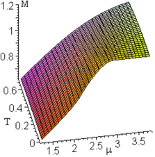
Figure 9: Magnetization of an electron gas in magnetic field, we put $\beta H=0.15E_{c}$, $\omega=0.3,\;\omega\acute{}=0.5i$ and $E_{c}=2.5$. Temperature and chemical potential take on dimensionless values, magnetization is measured in Bohr magnetons.

In Fig. 10, the graph $\partial_{\mu}^{2}M(T,\mu,H)$ on the temperature and the chemical potential is represented (while constructing, we used $\beta H=0.15E_{c}$, $\omega=0.3,\;\omega^{\prime}=0.5i$, accordingly $E_{c}=2.5$). One can see that when $\mu\rightarrow E_{c}\pm\beta H$ at $T=0$ the second derivative from the magnetic moment has infinite discontinuities and

$$\lim\limits_{\mu\rightarrow E_{c}-\beta H-0}\partial_{\mu}^{2}M_{0}=\infty,\;\lim\limits_{\mu\rightarrow E_{c}-\beta H+0}\partial_{\mu}^{2}M_{0}=const,$$

$$\lim\limits_{\mu\rightarrow E_{c}+\beta H-0}\partial_{\mu}^{2}M_{0}=-\infty,\;\lim\limits_{\mu\rightarrow E_{c}+\beta H+0}\partial_{\mu}^{2}M_{0}=const.$$

As in the previous case, the singularities at the points $E_{c}\pm\beta H$ smooth out slowly enough when the temperature increases.

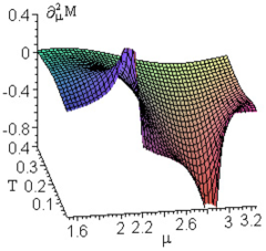
Figure 10: Second derivative of electron gas magnetization in magnetic field, we put $\beta H=0.15E_{c}$, $\omega=0.3,\;\omega\acute{}=0.5i$ and $E_{c}=2.5$. Temperature and chemical potential take on dimensionless values, magnetization is measured in Bohr magnetons. $\partial_{\mu}^{2}M(T,\mu,H)$ has infinite discontinuities when $\mu\rightarrow E_{c}\pm\beta H,\>T=0$.

VI Conclusions

In this paper, we have examined the one-gap and two-gap separable Lame potentials in detail. We have constructed the dispersion relation $E(k)$ for one-dimensional case and the Fermi surfaces in the first and second bands for three-dimensional case. The pictures illustrate a passage from the limit case of free electrons to the limit case of tight binding electrons. We have provided also analytical expressions for effective masses of electrons in a metal. These expressions depend on all the band edges.

These results have been used to study the singularities of the electron part of the thermodynamic characteristics in metals. We have derived explicit analytical expressions for the density of states in a metal and its derivative. Then we have examined the thermodynamic potential and magnetic moment of metal in an external magnetic field and extracted the singular part. We have also obtained the relation between the parameter of singularity and corresponding effective mass. All the expressions we derived contain the parameters of our potential only. Therefore, if we fix potential, we can calculate all the coefficients of these expressions.

It is necessary to point out that instead of electrons, the arbitrary quasi-particles can be considered within a framework of this approach.

We would like also to say a few words about generalization of the finite-gap potentials to lattices of other spacial symmetry. In the paper BD the authors have tried to develop such a generalization for HCP lattice by means of the perturbation theory and calculated the Fermi surface of Beryllium. The elliptic Calogero-Moser potentials are also of significant interest concerning their use in solid state physics. These potentials are multidimensional.