Distributions of switching times of single-domain particles using a time quantified Monte Carlo method

Abstract

Using a time quantified Monte Carlo scheme we performed simulations of the switching time distribution of single mono-domain particles in the Stoner-Wohlfarth approximation. We considered uniaxial anisotropy and different conditions for the external applied field. The results obtained show the switching time distribution can be well described by two relaxation times, either when the applied field is parallel to the easy axis or for an oblique external field and a larger damping constant. We found that in the low barrier limit these relaxation times are in very good agreement with analytical results obtained from solutions of the Fokker-Planck equation related to this problem. When the damping is small and the applied field is oblique the shape of the distribution curves shows several peaks and resonance effects.

I Introduction

The study of magnetic nanoparticles is very interesting from the theoretical and experimental point of view, in addition to its important technological applications in magnetic data storage. Magnetic media for data storage are composed of tiny magnetic grains, like magnetic particles, which have to be flipped in the magnetic recording process. Increasing the storage density implies a reduction in the size of the magnetic grains. If the grains are too small they lose thermal stability reaching the so called superparamagnetic limit. The stability problem can be overcome by increasing the anisotropy of the grains but then higher fields (which are difficult to reach in current devices) are needed to switch the magnetization in the recording process. In this sense a challenging issue about magnetization reversal arises which is how to have short reversal times, keeping the switching fields in small values Sun05PRB ; Sun06PRL and controlling the effects of thermal fluctuations. The thermal stability problem of ferromagnetic particles was first studied by Néel and then by Brown Neel49AG ; Brown63PR ; Brown79IEEE in the single spin approximation. Experimental studies for the switching time in a single magnetic nanoparticle Wernsdorfer97PRL ; Wernsdorfer97bPRL ; Thirion03N suggest in several cases the correctness of the Néel-Brown approximation.

In his work Brown Brown63PR derived the Fokker-Planck equation (FPE) for an assembly of particles using the stochastic Landau-Lifshitz-Gilbert dynamics (sLLG) and then obtained analytical expressions for the lowest eigenvalue of the Sturm-Liouville problem associated with the FPE in asymptotic cases. The lowest eigenvalue of the FPE is associated to the longer relaxation time which in several regimes is supposed to control the switching process. Since then several works have been done to obtain the lowest eigenvalue of FPE, with applied fields parallel Aharoni69PR and oblique Coffey95PRB ; Coffey98PRB to the easy axis. While in the past the attention was focused on the long time regime of the switching process, with the growing complexity of experimental devices and the need of ever smaller switching times, it turns to be desirable to have a knowledge of the whole process, from the earliest times to the longest ones, in order to explore alternative mechanisms for magnetization switching.

Since the FPE cannot be solved analytically except in limiting cases, the short relaxation times in the early stages of the switching process has to be studied by numerical integration of the sLLG Grinstein05PRB equation, or solving numerically the FPE. For the intermediate time scales numerical integration of Langevin dynamics is not useful since the small time step needed in the numerical integration does not allow to extend the simulation beyond the range of nanoseconds. In order to overcome this problem time quantified Monte Carlo methods (TQMC) were developed Nowak00PRL ; Smirnov-Rueda00JAP ; Chubykalo02JMMM ; Chubykalo03PRB that allow to extend the time span with a considerable gain in computational and programming efforts. In addition, Chubykalo et al. Chubykalo03PRB have also proved that these methods may be useful in the low damping condition, whenever the applied field is parallel to the anisotropy easy axis. However the method fails under an oblique applied field and low damping condition where precessional movement cannot be neglected. Recently, Cheng et al. Cheng06PRL mapped the sLLG dynamics and the Monte Carlo scheme through a Fokker-Planck approach introducing the precessional step in the TQMC simulations. With this improvement in principle TQMC simulations could be used also in the short times scales irrespectively of the configuration of the applied field and the value of the damping constant. However this improvement in the accuraccy is in detriment of the extent of time of the simulation. The situation is even worse when the system consists of a set of interaccting particles Cheng06PRB . Nevertheless, even in these cases the TQMC scheme seems a better alternative than solving numerically the sLLG equation. The main advantage is a far simpler implementation, whithout the need to control the stability of the algorithm as when solving a differential equation numerically. The second advantage is that, even though the gain in the time span simulated relative to the sLLG equation is certainly not as large as in the strong damping regime where precession can be ignored, the TQMC scheme allows to adjust the time step in a less constrained manner than the sLLG equation, resulting in a real gain in the total times that can be reached by the simulation. The extent of this gain depends on the particular problem considered.

In this work we used this approach to obtain the distribution of switching times in order to explore the incidence of short relaxation times in the switching process as a function of the damping and for different applied fields. We found that for external fields parallel to the easy axis the Brown approach works very well in practically the whole time span. The numerical results are extremely well described with only the two largest relaxation times from the solution of the Fokker-Planck equation. When the external field is oblique there are no analytical solutions available, except for the largest time scale. In this case, we found that two relaxation times are enough to describe the distribution of times when the damping is high. When the damping is low, the switching mechanism is dominated by precession, and the short time behavior is more complex, showing several peaks, which reflect the presence of different resonance frequencies.

II Theoretical Background

A single-domain particle can be modeled in the Stoner-Wohlfarth (SW) approximation where the magnetic state of the particle is described by a single magnetic moment $\vec{m}$ whose strength is equal to the total magnetic moment of the particle $|\vec{m}|=M_{s}v$. Here $M_{s}$ is the magnetization of saturation of the particle and $v$ is the particle volume. In the SW model the energy density $V$ of a particle with uniaxial anisotropy under an external applied field is expressed as:

$$-\beta V=\alpha[(\vec{n}\cdot\vec{s})^{2}+2\vec{h}\cdot\vec{s}],$$ (1)

here $\beta=v/k_{B}T$, $\vec{s}=\vec{M}/M_{s}$ and $\vec{n}$ are unit vectors defining the magnetization and the easy axis direction, respectively. The applied field $\vec{h}$ is expressed in reduced units $h=H/H_{k}$, with $H_{k}=2K/\mu_{0}M_{s}$ being the anisotropy field, $\alpha=Kv/k_{B}T$ is a dimensionless constant where $K$ is the anisotropy constant. In a classical approximation, the dynamics of a reduced magnetic moment $\vec{s}$ under thermal fluctuations is modeled by the stochastic Landau-Lifshitz-Gilbert (sLLG) equation,

$$\frac{d\vec{s}}{dt}=\frac{\gamma(\mu_{0}H_{k})}{1+a^{2}}\,\vec{s}\times[(\vec{h}_{eff}+\vec{h}_{fl})-\\ a\,\vec{s}\times(\vec{h}_{eff}+\vec{h}_{fl})],$$ (2)

where $\gamma$ is the gyromagnetic ratio, $a=\eta\gamma M_{s}$ is a dimensionless damping coefficient and $\eta$ is the damping coefficient in Gilbert’s equation. The effective field $\vec{h}_{eff}$ is given by the particle energy gradient,

$$\vec{h}_{eff}=-\frac{1}{2K}\frac{\partial V}{\partial\vec{s}}.$$ (3)

The stochastic fluctuating field $\vec{h}_{fl}$ is assumed as a Gaussian stochastic process with the following statistical properties:

$$<{h}_{fl,i}>=0,\,\,\,\,<h_{fl,i}(t)\,h_{fl,j}(s)>=\mu\,\delta_{i,j}\,\delta(t-s),$$ (4)

where $i$ and $j$ stand for the cartesian components.

In spherical coordinates, the FPE for the probability $W(\theta,\phi,t)$ of finding one the magnetic moment at time $t$ within a solid angle $d\Omega$ is given by Brown63PR ; Brown79IEEE :

$$\frac{\partial W}{\partial t}=\frac{1}{2\tau_{N}}\nabla^{2}W+ab\nabla^{2}V\,W+\frac{b}{\sin(\theta)}\left(\frac{\partial V}{\partial\theta}\frac{\partial W}{\partial\phi}-\frac{\partial V}{\partial\phi}\frac{\partial W}{\partial\theta}\right)$$ (5)

$$+ab\left(\frac{\partial V}{\partial\theta}\frac{\partial W}{\partial\theta}+\frac{1}{\sin(\theta)^{2}}+\frac{\partial V}{\partial\phi}\frac{\partial W}{\partial\phi}\right).$$

where the Néel time $\tau_{N}^{-1}=\mu\gamma^{2}(1+a^{2})$ is a characteristic diffusional time and $b=\gamma/(1+a^{2})M_{s}$. On the other hand, in order to satisfy the equilibrium statistical properties in the stationary regime,

$$\tau_{N}=\alpha\frac{(1+a^{2})}{a}\frac{1}{(\gamma\mu_{0}H_{K})}.$$ (6)

In general solutions of (5) can not be found analytically. However, the relaxation of any initial probability state can be formally described by a sum of exponentials:

$$W(\theta,\phi)=W_{0}+\sum_{n=1}^{\infty}A_{n}\,F_{n}(\theta,\phi)\,\exp(-t/\tau_{i}),$$ (7)

where $\tau_{i}$ are related to the eigenvalues of the Sturm-Liouville associated problem Brown63PR ; Aharoni69PR ; Coffey98PRB according to

$$\tau_{i}=\frac{2\tau_{N}}{\lambda_{i}}.$$ (8)

Besides the diffusional Néel time, the other characteristic time scales in this problem are the precessional time $\tau_{p}=(\gamma\mu_{0}H_{K}/(1+a^{2}))^{-1}$ and the damping time $\tau_{K}=\tau_{p}/a$ Garcia-Palacios98PRB . Then, eq. (8) expressed in terms of the damping times becomes $\tau_{i}[\tau_{K}]=\frac{2\alpha}{\lambda_{i}}$.

III Monte Carlo simulations

In our simulations we use a hybrid Monte Carlo method Nowak00PRL ; Cheng06PRL that emulates the stochastic dynamics of the LLG equation. This method combines the Metropolis or heat bath MC scheme with a random displacement of the magnetic moment within a cone Nowak00PRL and a precessional spin motion. The random displacement is obtained by adding to the normalized magnetic moment a random vector uniformly distributed within an sphere of radius $R\ll 1$ and then normalizing the resulting vector again, while the magnitude and direction of the precessional motion is given by

$$\Delta\vec{s}=-\Phi\ \vec{s}\times\vec{h}_{eff},$$ (9)

where $\Phi=\frac{\alpha}{10a}R^{2}$. In this MC scheme the magnetic moment update is chosen with equal probability between a precessional step and a random displacement. The acceptance rate $A(\beta\Delta V)$ of the random motion is based in the heat bath procedure,

$$A(\beta\Delta V)=1/[1+\exp(\beta\Delta V)].$$ (10)

By means of a detailed comparison between the Fokker-Planck equation representing the MC stochastic dynamics and the corresponding equation associated with the LLG micromagnetic equation, it is possible to obtain a very accurate mapping between Monte Carlo Steps and the real time scale from the LLG equation Cheng06PRL through the following relation:

$$\Delta t[\tau_{K}]=\frac{\alpha}{20}R^{2}\Delta t[MCS],$$ (11)

where the real time scale is expressed in units of the damping characteristic time $\tau_{K}$.

IV Results

We have performed numerical evaluations of the switching time distribution with the following protocol: we start with the magnetic moment pointing in the easy axis direction, in our case the $z$ axis, and then we apply an inverse magnetic field of different strengths and direction. The switching time is defined as the time required for the z component of the magnetic moment to change its sign. Since we want to compare our results with analytic predictions from the Fokker-Planck equation 5, we count every time the magnetic moment crosses the equatorial line, i.e., we compute the whole probability that the magnetic moment attains an angle $\theta=\pi/2$ in a given time $t$. Otherwise we would be computing the first passage time, for which there are still less analytic results available. We performed $10^{6}$ realizations to obtain the switching time distribution $P(t)$. Since $P(t)\propto\int_{0}^{2\pi}W(\theta=\pi/2,\phi,t)\,d\phi$, it has the same relaxational behavior than $W(\theta,t)$.

In order to test the confidence of our results we simulated switching times distribution for the low barrier limit ($\alpha<1$), with the applied field parallel to the easy axis. In this case the two smallest eigenvalues are given by Brown63PR ,

$$\lambda_{1}=2-\frac{4}{5}(1-h^{2}\alpha)\alpha+\frac{96}{875}\alpha^{2}+\vartheta(\alpha^{3})$$ (12)

$$\lambda_{2}=6-\frac{4}{7}(1-h^{2}\alpha)\alpha+\frac{64}{343}\alpha^{2}+\vartheta(\alpha^{3}).$$

From equations (8) and (11), and considering that a time of $3\tau_{1}$ is enough to obtain a complete distribution curve, the number of MCS that should be used for each realization is:

$$\Delta t[MCS]=\frac{60}{R^{2}\lambda_{i}}.$$ (13)

In the simulations we used $R=0.03$, which is a good compromise between accuracy and efficiency. In figure 1 we present the switching time distribution for an external field $h=0.292$ parallel to the easy axis and low energy barrier $\alpha=1$. At short times the probability that the particle switches is zero since there is a minimal time necessary to surmount the barrier. Except for the very short times, the distribution is well fitted using two exponentials $P(t)=a_{0}+a_{1}\exp(-t/\tau_{1})+a_{2}\exp(-t/\tau_{2})$ where the relaxation times $\tau_{1}$ and $\tau_{2}$ are obtained through eq. (8) using the eigenvalues given in eqs. (12). We can see that two relaxation times are enough to obtain a good fit of the switching time distribution in a wide range and a very good agreement for the relaxation times obtained through the FPE. The switching time distribution at large times is finite because the energy barrier is small and the particle attains thermodynamic equilibrium with a finite probability of being at $\theta=\pi/2$.

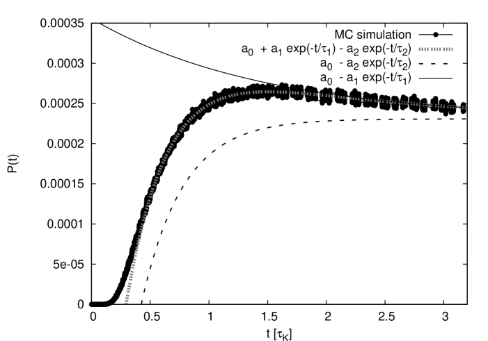
Figure 1: Switching time distribution in the low barrier case $\alpha=1$ and parallel applied field $h=0.292$, here the damping constant is $a=1$. The relaxation times used in the fitting $\tau_{1}=7.71$ and $\tau_{2}=1.79$ are obtained from eqs. (8) and (12).

In fig. 2, the energy barrier is increased ($\alpha=10$) keeping the field parallel, with $h=0.4$. In this case the switching time distribution has a peak before relaxing to zero. In this case the distribution goes to zero at large times since the magnetic moment gets trapped in the deepest minimum A similar behavior is found by integrating the sLLG equation Grinstein05PRB . Like in fig. 1, this curve is well fitted by two relaxation times. The longer time $\tau_{1}$ used in this fitting corresponds to results of Coffey et al. Coffey98PRB . The secondary relaxation time $\tau_{2}$ , which is supposed to be related to the second eigenvalue is much lower than $\tau_{1}$ and is important in the very first stages of the relaxation, having little influence in the switching mean time $<t>$. We also show in fig. 2 two curves corresponding to small and large damping constants $a=0.1,\,100$. These curves are indistinguishable within the statistical error, when plotted in units of the damping time $\tau_{K}$. This is because if the applied field is parallel to the easy axis, then the potential energy has azimuthal symmetry and the precessional motion, which is important for small damping, has no influence in crossing the barrier. We will see below that a different situation is observed if the applied field is oblique. However, from the point of view of the Monte Carlo simulation, the damping constant has a critical influence since the precessional factor $\Phi$ has to be kept at small values in order to correctly follow the trajectory. Then, reducing the damping constant implies a reduction of $R$ in eq. (9), and the number of MCS required in the simulation notably increase (see eq. (13)).

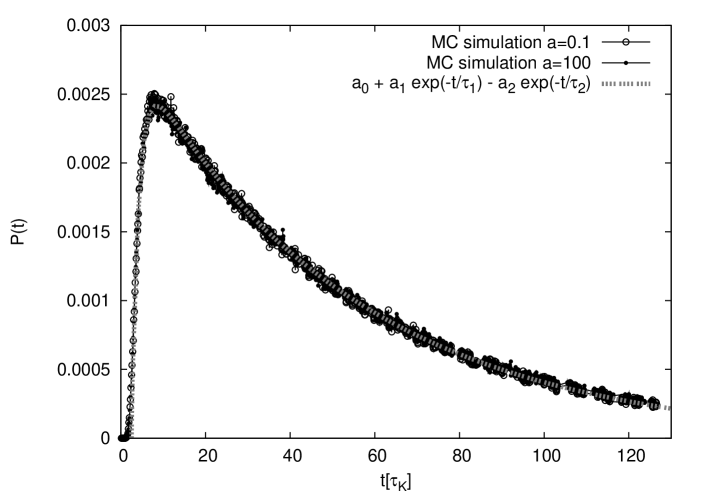
Figure 2: High barrier switching time distribution with $\alpha=10$ for two damping constants $a=0.1$ and $100$ and parallel applied field $h=0.4$. The longer relaxation time $\tau_{1}=52.0$ is obtained from table I Coffey98PRB . The secondary relaxation time is obtained from fitting: $\tau_{2}=1.72$ and the mean time $t_{m}=42.5$.

Figure 3 is similar to fig. 2, $h=0.4$, but now the applied field is at an angle of $\pi/4$ with respect to easy axis. The damping constant has now influence on the switching behavior, this is due to the coupling between the longitudinal and normal modes Kalmykov04JAP . When the applied field is oblique the particle crosses the barrier through a saddle point and the precessional motion influences the way the energy landscape is explored. If the damping constant is high the particle tends to relax to the nearest minimum and only through thermal fluctuations the saddle point can be found, wheres if the damping constant is kept small, precessional motion affects the switching process. Note that a shoulder is present after the first peak in the case of small damping.

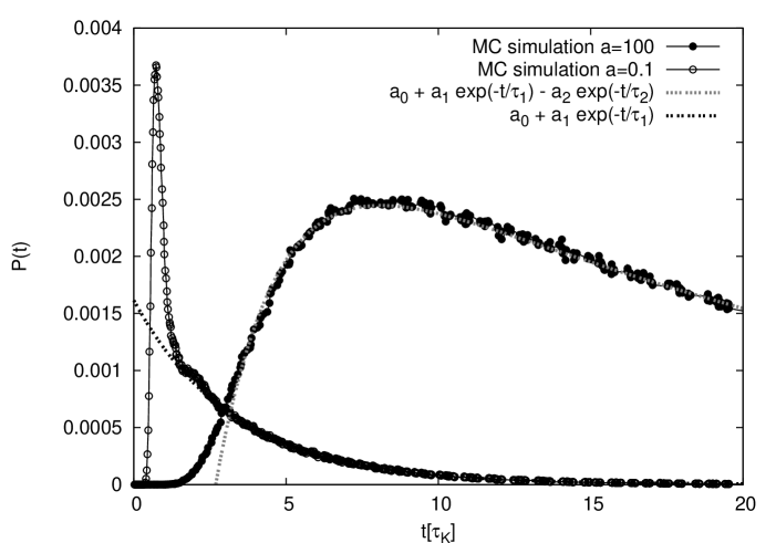
Figure 3: High energy barrier $\alpha=10$ under an oblique applied field $\phi=\pi/4,\,h=0.4$ for two different values of the damping constant $a=0.1,\,100$. It can be seen that in the larger damping case the distribution is well described by two relaxation times whereas in the low damping case a secondary peak appears.

In fig. 4 the damping constant is decreased even more to $a=0.01$. Now new peaks appear in the switching time distribution, which shows resonance-like effects. If the starting energy is similar to the energy of the saddle point and the damping constant is low enough, the particle does not relax quickly and keeps its energy nearly constant for a long time, letting the magnetic moment to cross the equatorial line more than one time. This behavior is analyzed in more detail in figure 5, where the curve of fig. 4 is plotted together with the distribution of the first and second passage times. The figure shows that the first and second peaks in the switching time distribution correspond to the main peaks of the first and second passage times distributions, respectively. These distributions show also secondary peaks, which probably correspond to different paths of switching in the energy landscape. From the figure is also clear that the first passage time probability goes to zero at $t/\tau_{K}\approx 70$, while the whole distribution stays finite until much longer times. This fact means that the magnetic moment can go back and forth across the saddle point and the magnetic moment keeps switching between the basins of the two minima during a long time. Although the barrier is high, the small damping makes the magnetic moment to follow a long trajectory before settling in the final state.

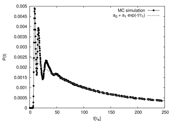
Figure 4: Switching time distribution for a very low damping value $a=0.01$. Like in fig. 3 here $\alpha=10$, $\phi=\pi/4$ and $h=0.4$. We can see at least four peaks and an exponential relaxing behavior at the longest times.

Figure 5: Switching time distribution of fig. 4 together with the first and second passage time distribution. Clearly the first and second peak of the total distribution correspond to the first a second passage, respectively.

V Summary

In summary, by performing Monte Carlo simulations including a precessional step, we have obtained switching time distributions of magnetic particles in the Stoner-Wolfarth limit, for different configurations of the applied field, different values of the damping constant and different heights of the energy barriers. We conclude that if the damping constant is high enough the distributions are well described by two relaxation times associated with the eigenvalues of the Fokker-Planck solutions of the corresponding Landau-Lifshitz-Gilbert dynamics, irrespectively of the configuration of the applied field. If the damping constant takes small values and the applied field is oblique to the anisotropy axis, the distributions show resonance effects, evidencing the importance of the precessional motion in the inversion mechanism. The present Monte Carlo algorithm allows to study these precessional effects in detail, without the need to solve the LLG equations. We showed that the first two peaks in the distribution functions correspond to the first and second passage times of the magnetization through the equator. In all cases the characteristic inversion time is given by the smallest eigenvalue of the FPE, while in the cases with strong damping the whole distribution can be very well described by only two relaxation times.

VI Acknowledgments

This work was partially supported by grants from FAPERGS and CNPq (Brazil), and by grants from CONICET and SECYT/UNC (Argentina).

References

- (1) Z. Z. Sun, X. R. Wang, Fast magnetization switching of stoner particles: A nonlinear dynamics picture, Phys. Rev. B 71 (2005) 174430.
- (2) Z. Z. Sun, X. R. Wang, Theoretical limit of the minimal magnetization switching field and the optimal field pulse for stoner particles, Phys. Rev. B 97 (2006) 077205.
- (3) L. Nèel, Théorie du traînage magnétique des ferromagnétiques en grains fins avec application aux terres cuites, Ann, Géophys. 5 (1949) 99–136.
- (4) J. William Fuller Brown, Thermal fluctuations of a single-domain particle, Phys. Rev. 130 (1963) 1677–1686.
- (5) J. William Fuller Brown, Thermal fluctuations of fine ferromagnetic particles, IEEE Transactions on Magnetism 15 (5) (1979) 1196–2008.
- (6) W. Wernsdorfer, E. B. Orozco, K. Hasselbach, A. Benoit, B. Barbara, N. Demoncy, A. Loiseau, H. Pascard, D. Mailly, Experimental evidence of the néel-brown model of magnetization reversal, Phys. Rev. Lett. 78 (9) (1997) 1791–1794.
- (7) W. Wernsdorfer, E. B. Orozco, K. Hasselbach, A. Benoit, D. Mailly, O. Kubo, H. Nakano, B. Barbara, Macroscopic quantum tunneling of single ferromagnetic nanoparticles of barium ferrites, Phys. Rev. Lett. 79 (20) (1997) 4014–4017.
- (8) C. Thirion, W. Wernsdorfer, D. Mailly, Switching of magnetization by nonlinear resonance studied in single nanoparticles, Nature Materials 2 (2003) 524–527.
- (9) A. Aharoni, Effect of a magnetic field on the superparamagnetic relaxation time, Phys. Rev. 177 (2) (1969) 793–796.
- (10) W. T. Coffey, D. S. F. Crothers, J. L. Dormann, L. J. Geoghegan, Y. P. Kalmykov, J. T. Waldron, A. W. Wickstead, Effect of an oblique magnetic field on the superparamagnetic relaxation time, Phys. Rev. B 52 (22) (1995) 15951–15965.
- (11) W. T. Coffey, D. S. F. Crothers, J. L. Dormann, L. J. Geoghegan, E. C. Kennedy, Effect of an oblique magnetic field on the superparamagnetic relaxation time. ii influence of the giromagnetic term, Phys. Rev. B 58 (6) (1998) 3249–3266.
- (12) G. Grinstein, R. H. Koch, Switching probabilities of single-domain magnetic particles, Phys, Rev. B 71 (2005) 184427–4.
- (13) U. Nowak, R. W. Chantrell, E. C. Kennedy, Monte carlo simulations with step quantification in terms of langevin dynamics, Phys. Rev. Lett. 84 (2000) 163.
- (14) R. Smirnov-Rueda, O. Chubykalo, U. Nowak, R. W. Chantrell, J. M. Gonzalez, Real time quantification of monte carlo steps for different time scales, J. Appl. Phys. 87 (9) (2000) 4798.
- (15) O. Chubykalo, J. Kauffman, B. Lengsfield, R. Smirnov-Rueda, Long-time calculation of the thermal magnetization reversal using metropolis monte carlo, J. Magn. Magn. Mater. 242-245 (2002) 1052.
- (16) O. Chubykalo, U. Nowak, R. Smirnov-Rueda, M. A. Wongsam, R. W. Chantrell, J. M. Gonzalez, Monte carlo technique with a quantified time step: Application to the motion of magnetic moments, Phys. Rev. B 67 (2003) 064422.
- (17) W. T. Cheng, M. B. A. Jalil, H. K. Lee, Y. Okabe, Mapping the monte carlo scheme to langevin dynamics: A fokker-planck approach, Phys. Rev. Lett. 96 (2006) 067208.
- (18) W. T. Cheng, M. B. A. Jalil, H. K. Lee, Time-quantified monte carlo algorithm for interacting spin array micromagnetic dynamics, Phys. Rev. B 73 (2006) 224438.
- (19) J. L. Garcia-Palacios, F. J. Lázaro, Langevin-dynamics study of the dynamical properties of small magnetic particles, Phys. Rev. B 58 (22) (1998) 14 937–14 958.
- (20) P. K. Yuri, The relaxation time of the magnetization of uniaxial single-domain ferromagnetic particles in the presence of a uniform magnetic field, J. Appl. Phys. 96 (4) (2004) 1138.