Fermi Liquid Theory of a Fermi Ring

Abstract

We study the effect of electron-electron interactions in the electronic properties of a biased graphene bilayer. This system is a semiconductor with conduction and valence bands characterized by an unusual “mexican-hat” dispersion. We focus on the metallic regime where the chemical potential lies in the “mexican-hat” in the conduction band, leading to a topologically non-trivial Fermi surface in the shape of a ring. We show that due to the unusual topology of the Fermi surface electron-electron interactions are greatly enhanced. We show that the ferromagnetic instability can occur provided a low density of carriers. We compute the electronic polarization function in the random phase approximation and show that, while at low energies the system behaves as a Fermi liquid (albeit with peculiar Friedel oscillations), at high frequencies it shows a highly anomalous response when compare to ordinary metals.

I Introduction

The discovery of graphene Exp , and the realization that it presents very unusual electronic properties Peres06 , has generated an enormous amount of interest in the condensed matter community. The possibility of creating electronic devices consisting of only a few atomic layers can open doors for a carbon-based micro-electronics. In this context, bilayer systemsMcCannFalko play a distinguished role for being the minimal system to produce a gap in the electronic spectrum due to an electric field effect McCann ; GNP06 . Recent experiments show that the electronic gap and the chemical potential can be tuned independently of each other and the band structure can be well described by a tight-binding model corrected by charging effects eduardo . The electronic gap in these systems has been observed recently in angle resolved photoemission (ARPES) Ohta in epitaxially grown graphene films on SiC crystal surfaces walt .

Electron-electron interactions are usually neglected in single layer graphene since they do not seem to play an important role in the transport measurements in low magnetic fields, e. g., in the measurements of the anomalous quantum Hall effect qhe . At high magnetic fields, however, the electronic kinetic energy becomes quenched by the creation of Landau levels kim and Coulomb interactions become important allan ; Herbut06 . An alternative theory predicts that Coulomb interaction becomes relevant even at arbitrary small magnetic fields Herbut06 . Also, the minimal conductivityMish06 and collective excitationsHwang06 depend on the electron-electron interaction.

In single graphene sheets, the unscreened electron-electron interaction is - due to the vanishing density of state at the Dirac point - marginally irrelevant in the renormalization group sense. This leads to a behavior with the electronic self-energy of the form, $\text{Im}\Sigma\propto\omega$, Gon96 which is reminiscent of so-called marginal Fermi liquid behavior note . The fact that even the unscreened Coulomb interactions are marginally irrelevant in single layer graphene suppresses the presence of magnetic phases in this system. In fact, ferromagnetism can only be found in strong coupling, when graphene’s fine structure constant, $\alpha_{G}=e^{2}/(\epsilon_{0}\hbar v_{F})$ ($e$ is electric charge, $\epsilon_{0}$ is the dielectric constant, and $v_{F}$ is the Fermi-Dirac velocity), is larger than a critical value $\alpha_{c}$. It was found that $\alpha_{c}\approx 5.3$ for clean graphene ($\alpha_{c}\approx 3.8$ for disordered graphene) Peres05 . For $\epsilon_{0}=1$ we have $\alpha_{G}\approx 2$ which is smaller than the critical value indicating the absence of a ferromagnetic transition in single layer graphene. For Coulomb effects in disordered graphene, see also Refs. Sta05, .

In this paper, we study the electron-electron interaction in the biased bilayer system (or unbiased graphene bilayer see Ref. Wang07 ). We use the standard tight-binding description of the electronic structure McClure and treat the problem in the metallic regime when the chemical potential lies in the conduction band leading to a topologically non-trivial ring for the Fermi surface. We also disregard inter-band transitions by assuming that the electronic gap is sufficiently large so that the valence band is completely filled and inert. We show that the ferromagnetic instability can occur in this system due to the reduced phase space of the ring. We also calculate the polarization properties of this system and show that they are rather unusual at high frequencies with peculiar Friedel oscillations at low frequencies.

The paper is organized as followed. In section II, we introduce the model and discuss the self-energy effects due to electron-electron interactions. In section III, we present a discussion of the stability of the system towards ferromagnetism by introducing a Landau-Ginzburg functional for the free energy. In section IV, we calculate two-particle correlation functions, i.e., the imaginary part of the polarization and the plasmon dispersion. We close with conclusions and future research directions.

II The effective model

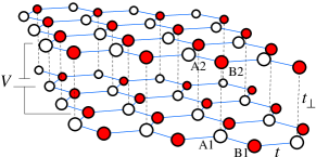
Figure 1: (Color online) Lattice structure of a bilayer graphene. The A and B sublattices are indicated by white and red spheres, respectively.

The graphene bilayer consists of two graphene planes (labeled $1$ and $2$), with a honeycomb lattice structure, and stacked according to Bernal order (A1-B2), where A and B refer to each sublattice of a single graphene (see Fig. 1). The system is parameterized by a tight-binding model for the $\bm{\pi}$-electrons with nearest-neighbor in-plane hopping $t$ ($\approx 2.7$ eV) and inter-plane hopping $t_{\perp}$ ($\approx 0.3$ eV). The two layers have different electrostatic potentials parameterized by $V$. The electronic band structure of the biased bilayer is obtained within the tight-binding description eduardo , leading to the dispersion relation (we use units such that $\hbar=1=k_{B}$):

$$E_{\mathbf{k}}^{\pm\pm}(V)\!\!=\!\!\pm\sqrt{\!\epsilon_{\mathbf{k}}^{2}\!+\!t_{\perp}^{2}/2\!+\!V^{2}/4\!\pm\!\sqrt{\!t_{\perp}^{4}/4+(t_{\perp}^{2}\!+\!V^{2}\!)\epsilon_{\mathbf{k}}^{2}}}\,,$$ (1)

where $\epsilon_{\mathbf{k}}$ is the dispersion of a single graphene layer,

$$\epsilon_{\mathbf{k}}=t[3+2\cos(ak_{x})+4\cos\left(ak_{x}/2\right)\cos\left(ak_{y}\sqrt{3}/2\right)]^{1/2}\,,$$ (2)

where ${\bf k}=(k_{x},k_{y})$ is the two-dimensional (2D) momentum. This dispersion relation around the $K$ and $K^{\prime}$ points of the Brillouin zone are shown in Fig. 2. Notice that the electronic spectrum shows a “mexican-hat” dispersion with a gap minimum, $\Delta_{g}$, given by:

$$\Delta_{g}=V[t_{\perp}^{2}/(t_{\perp}^{2}+V^{2})]^{1/2}\,,$$ (3)

that is located at momentum $k_{0}$ relative to the $K$ point. Close to the $K$ point the electronic dispersion can be written as:

$$E(\bm{k})\approx\Delta-\alpha k^{2}+\lambda k^{4}\,,$$ (4)

where

$$\Delta = \frac{V}{2}\,,$$

$$\alpha = \frac{V}{t_{\perp}^{2}}v_{F}^{2}\,,$$

$$\lambda = V\left(\frac{(t^{2}_{\perp}+V^{2})^{2}}{V^{2}t^{6}_{\perp}}-\frac{1}{t^{4}_{\perp}}\right)v_{F}^{4}\,,$$ (5)

where $v_{F}=3ta/2$ where $a=1.41$Å is the lattice-spacing. The energy dispersion (4) has the shape shown in Fig. 3, with its minimum at momentum

$$k_{0}=\sqrt{\alpha/(2\lambda)}\,.$$ (6)

For a finite density of electrons in the conduction band the occupied momentum states are constrained such that $k_{\rm min,\sigma}<k<k_{\rm max,\sigma}$ where:

$$k^{2}_{\rm min,\sigma} = \frac{\alpha}{2\lambda}-2\pi n_{\sigma}\,,$$ (7)

$$k^{2}_{\rm max,\sigma} = \frac{\alpha}{2\lambda}+2\pi n_{\sigma}\,,$$ (8)

where $n_{\sigma}$ is the electronic density per unit area for electrons with spin $\sigma=\pm 1$.

The density of states per unit area $\rho(\epsilon)$ can be written as:

$$\rho(\epsilon)=\frac{1}{4\pi\sqrt{\lambda}}\frac{1}{\sqrt{\epsilon-\epsilon_{\rm min}}}\,,$$ (9)

with $\epsilon_{\rm min}=\Delta-\alpha^{2}/(4\lambda)$, which has a square root singularity at the band edge, just like in one-dimensional (1D) systems. This 1D singularity in the density of states of the biased bilayer leads to an strong enhancement in the electron scattering either by other electrons or impurities (which is beyond the scope of this paper). The Fermi energy, $\epsilon_{F}$, can be expressed in terms of the electronic density per unit area, $n_{\sigma}$, as

$$\epsilon_{F}=\epsilon_{\rm min}+(2\pi n_{\sigma}\sqrt{\lambda})^{2}\,.$$ (10)

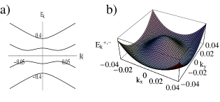
Figure 2: a) The four bands $E_{{\bf k}}^{\pm,\pm}$ (in eV) as function of $|{\bf k}|$ (in Å^-1) around the $K$ point with $V=t_{\perp}$. b) The “mexican-hat” $E_{{\bf k}}^{+,-}$ (in eV) as function of ${\bf k}$ (in Å^-1) around the $K$ point.

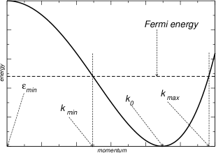
Figure 3: “Mexican-hat” dispersion of the biased graphene bilayer close to the $K$ point in the Brillouin zone. The symbols are explained in the text.

The simplest model including the effect of electron-electron interactions in this problem is:

$$H =\sum_{\bm{k},\sigma}E(\bm{k})c^{\dagger}_{\bm{k},\sigma}c_{\bm{k},\sigma}$$ (11)

$$+\frac{1}{2A}\sum_{\bm{k},\bm{p},\bm{q}}\sum_{\sigma,\sigma^{\prime}}V(q)c^{\dagger}_{\bm{k}+\bm{q},\sigma}c^{\dagger}_{\bm{p}-\bm{q},\sigma^{\prime}}c_{\bm{p},\sigma^{\prime}}c_{\bm{k},\sigma}\,,$$

where $c_{\bm{k},\sigma}$ ($c^{{\dagger}}_{\bm{k},\sigma}$) annihilates (creates) and electron with momentum $\bm{k}$ and spin $\sigma$. Notice that only the Coulomb interaction between the electrons of the occupied conduction band is considered. The Fourier transform of the Coulomb potential is given by:

$$V(q)=\frac{2\pi e^{2}}{\epsilon_{0}q}\,.$$ (12)

The unperturbed electronic Green’s function reads:

$$G^{0}(\bm{k},i\omega_{n})=[i\omega_{n}-E(\bm{k})]^{-1}\,,$$ (13)

where $\omega_{n}=(2n+1)\pi/\beta$ are fermionic Matsubara frequencies.

II.1 First order corrections to the quasi-particle spectrum

Figure 4: Evaluated diagrams where the solid line resembles the bare electronic propagator and the wiggled line the bare Coulomb interaction: a) electronic self-energy. b) particle-hole bubble or polarization.

The first order correction to the electronic self-energy is given by the diagram in Fig. 4 (a), and it reads:

$$\Sigma_{1}(\bm{k})=-\frac{2\pi e^{2}}{\epsilon_{0}A}\sum_{\bm{q}}\frac{1}{\beta}\sum_{n}\frac{1}{q}G^{0}(\bm{k}-\bm{q},i\omega_{n})\,,$$ (14)

and considering the zero temperature limit, one gets

$$\Sigma_{1}(\bm{k}) = -\frac{e^{2}k_{\rm max}}{2\pi\epsilon_{0}}I_{1}(a,k/k_{\rm max})\,,$$

$$\simeq -\frac{e^{2}k_{\rm max}}{2\pi\epsilon_{0}}\Big{[}2(1-a)\pi+\frac{1}{2}\left(\frac{1}{a}-1\right)\pi\frac{k^{2}}{k^{2}_{\rm max}}$$

$$\quad\quad\quad+\frac{3}{32}\left(\frac{1}{a^{3}}-1\right)\pi\frac{k^{4}}{k^{4}_{\rm max}}\Big{]}\;,$$

where $a=k_{\rm min}/k_{\rm max}$ and the Coulomb integral $I_{1}(x)$ is given in appendix A. From this result one obtains the renormalized values for $\Delta$, $\alpha$ and $\lambda$, defined as $E_{1}(\bm{k})=E(\bm{k})+\Sigma_{1}(\bm{k})$. For $k_{\rm min}>0$, i.e., the Mexican hat is partially filled, the renormalized values read

$$\Delta_{1} =\Delta-\frac{e^{2}}{\epsilon_{0}}(k_{\rm max}-k_{\rm min})\,,$$ (16)

$$\alpha_{1} =\alpha+\frac{e^{2}}{4\epsilon_{0}}\left(\frac{k_{\rm max}-k_{\rm min}}{k_{\rm max}k_{\rm min}}\right)\,,$$ (17)

$$\lambda_{1} =\lambda-\frac{3e^{2}}{64\epsilon_{0}}\left(\frac{k^{3}_{\rm max}-k^{3}_{\rm min}}{k^{3}_{\rm max}k^{3}_{\rm min}}\right)\,.$$ (18)

A consequence of the renormalization of the bare parameters is that for densities such that $\lambda_{1}\leq 0$, the spectrum becomes unbounded indicating the a possible instability of the non-interacting system. For realistic values of the parameters (see Section III), the instability occurs at $k_{\rm min}/k_{0}\approx 3/4$, i.e., for densities close to $n_{\sigma}\approx n_{\sigma}^{c}=k_{0}^{2}/(2\pi)$ when the Mexican hat is completely filled. We will confine ourselves to the limit of low densities so that the expansion of the energy dispersion in Eq. (4) up to the quartic term in the electron dispersion is valid. For larger densities for which $\lambda_{1}\approx 0$, higher order terms in the expansion must be included. For $n_{\sigma}\geq n_{\sigma}^{c}$, i.e., the Mexican hat is completely filled, the electron-electron interaction stabilizes the dispersion and the dip in the spectrum reduces. In this case, the parameters of the model modify to:

$$\Delta_{1} =\Delta-\frac{e^{2}}{\epsilon_{0}}k_{\rm max}\;,$$ (19)

$$\alpha_{1} =\alpha-\frac{e^{2}}{4\epsilon_{0}}k_{\rm max}^{-1}\;,$$ (20)

$$\lambda_{1} =\lambda+\frac{3e^{2}}{64\epsilon_{0}}k_{\rm max}^{-3}\;.$$ (21)

III Exchange instability of the ground state

In this section we examine a possible instability of the Fermi ring is unstable towards a ferromagnetic ground state. For the instability to occur, the exchange energy due to Coulomb interactions has to overcome the loss of kinetic energy when the system is polarized. The kinetic energy for electrons of spin $\sigma$ has the form:

$$K_{\sigma}(n,m)=\frac{A}{2\pi}\left[\left(2\pi\Delta-\frac{\pi}{2}\frac{\alpha^{2}}{\lambda}\right)n_{\sigma}+\frac{8}{3}\lambda\pi^{3}n_{\sigma}^{3}\right]\;,$$ (22)

where $A$ is the area of the bilayer. The exchange energy for electrons with spin $\sigma$ can be written as

$$E_{\sigma}^{\rm Exc}=\frac{1}{2A}\sum_{\rm k,\rm k^{\prime}\text{ occup.}}V(|\rm k-\rm k^{\prime}|)|\langle\rm k|\rm k^{\prime}\rangle|^{2}\;.$$ (23)

Within the approximations described in the introduction, i.e., assuming that the wave functions are mostly localized on one sublattice in one layer, the overlapp factor $\langle\rm k|\rm k^{\prime}\rangle\approx 1$. This leads to

$$E_{\sigma}^{\rm Exc}(n,m)=-\frac{e^{2}A}{8\pi^{2}\epsilon_{0}}k^{3}_{{\rm max},\sigma}\,I_{2}\left(\frac{k_{{\rm min},\sigma}}{k_{{\rm max},\sigma}}\right)\,,$$ (24)

where $k_{{\rm max},\sigma}$ and $k_{{\rm min},\sigma}$ are defined in Eqs. (7) and (8), (see Fig. 3).

In the paramagnetic phase both spin bands have the same number of electrons and hence $n_{\sigma}=n/2$. In the ferromagnetic phase the system acquires a magnetization density, $m=n_{+}-n_{-}$, and the electron occupation change to: $n_{\sigma}=(n+\sigma m)/2$. In order to study a possible ferromagnetic transition, we derive a Landau-Ginzburg functional in powers of $m$, with the coefficients depending on $n$. The Landau-Ginzburg functional is defined as:

$$F[\alpha,\lambda,n,m] =\sum_{\sigma}[K_{\sigma}(n,m)+E_{\sigma}^{\rm Exc}(n,m)$$ (25)

$$\quad\quad-K_{\sigma}(n,0)-E_{\sigma}^{\rm Exc}(n,0)]$$

$$\simeq a(n)m^{2}+b(n)m^{4}+c(n)m^{6}+\ldots\,.$$

A second order magnetic transition occurs when $a(n)$ becomes negative. If $a(n)$ is always positive, a first order transition may occur if $b(n)$ becomes negative. The term linear in $n_{\sigma}$ in the kinetic energy (22) does not contribute to $F[\alpha,\lambda,n,m]$.

The coefficient $a(n)$ has two main contributions: one comes from the kinetic energy (22), $a^{K}(n)$, and another arises from the exchange (24), $a^{\rm ex}(n)$. These contributions read:

$$a^{K}(n) =A\lambda\pi^{2}n\,,$$ (26)

$$a^{\rm ex}(n) =-\frac{e^{2}A}{4\epsilon_{0}}(L_{0}+L_{1}+L_{2})\,,$$ (27)

where the coefficients $L_{i}$ are functions related to the Coulomb integral $I_{2}(x)$ defined in appendix A in the following way:

$$L_{0} =\frac{3}{8}k^{-1}_{\rm max}I_{2}\left(\frac{k_{\rm min}}{k_{\rm max}}\right)$$

$$L_{1} =-\frac{3}{2}\frac{k^{2}_{0}}{k^{2}_{\rm max}\,k_{\rm min}}I^{{}^{\prime}}_{2}\left(\frac{k_{\rm min}}{k_{\rm max}}\right)$$

$$L_{2} =\frac{k_{0}^{4}}{2k^{3}_{\rm max}\,k^{2}_{\rm min}}I^{{}^{\prime\prime}}_{2}\left(\frac{k_{\rm min}}{k_{\rm max}}\right)+\frac{k_{0}^{2}(k^{2}_{0}-2n\pi)}{2k^{2}_{\rm max}\,k^{3}_{\rm min}}I^{{}^{\prime}}_{2}\left(\frac{k_{\rm min}}{k_{\rm max}}\right)$$

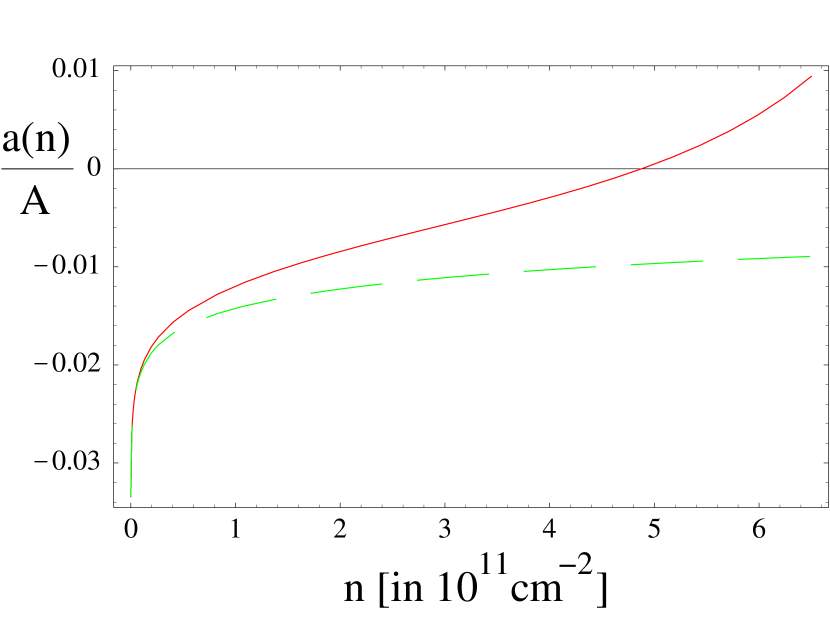
Figure 5: (Color online): Plot of $a(n)/A$ (in units of eV$[10^{11}\text{cm}^{-2}]^{-1}$), as function of the electronic density $n$ (in units of $10^{11}\text{cm}^{-2}$). The dashed (green) line gives the bare value of $a(n)/A$, the full (red) line contains self-energy corrections.

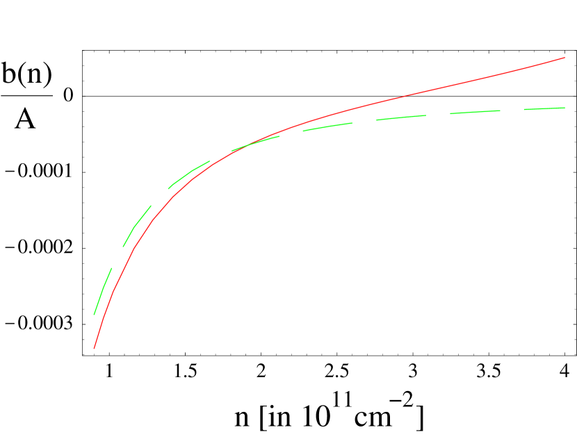
Figure 6: (Color online): Plot of $b(n)/A$ (in units of eV$[10^{11}\text{cm}^{-2}]^{-3}$), as function of the electronic density $n$ (in units of $10^{11}\text{cm}^{-2}$). The dashed (green) line gives the bare value, the full (red) line is the result with self-energy corrections.

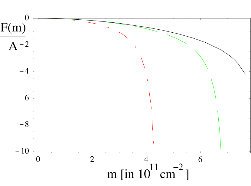
Figure 7: (Color online): Plot of $F(m)/A$ (in units of eV$[10^{11}\text{cm}^{-2}]$), as function of the magnetic density $m$ (in units of $10^{11}\text{cm}^{-2}$) for various electronic densities $n$ including self-energy corrections. The dotted-dashed (red) line stands for $n=5\times 10^{11}\text{cm}^{-2}$, the dashed (green) line for $n=2.5\times 10^{11}\text{cm}^{-2}$ and the full (black) line for $n=10^{11}\text{cm}^{-2}$.

In the following, we choose the parameters as in section II with $V=t_{\perp}$. For $\alpha_{G}\approx 2$ all coefficients are negative indicating that the system has a strong tendency towards ferromagnetic ordering. In this case the transition is of second order. There are, however, values of $\alpha_{G}$ for which $a(n)$ is positive, whereas the remaining coefficients are negative. In this case the transition is of first order. At zero temperature the magnetization density equals the density of electrons.

We have also investigated how the above picture changes if one includes the corrections to energy spectrum due to the electron-electron interaction, given by Eqs. (17) to (18). The comparison is shown in Fig. 5 and Fig. 6 where the dashed line shows the coefficients without self-energy effects whereas the full line includes self-energy effects. The inclusion of self-energy effects decreases the tendency toward a ferromagnetic ground-state and there is a critical density for which both coefficients, $a(n)$ and $b(n)$, become positive. This is also seen in Fig. 7, where the free energy $F(m)$ is shown for various electronic densities. Including self-energy effects leads to the saturation of the magnetization at high densities, i.e., for $n=5\times 10^{11}\text{cm}^{-2}$ the magnetization is not given by $m=n$ but by a lower value. Nevertheless, at low densities ($n\leq 10^{11}\text{cm}^{-2}$) the picture is not modified by self-energy corrections and we expect ferromagnetic ordering at $T=0$.

IV Polarization

In this Section, we calculate the bilayer density-density correlation function, i.e., the response of the system to an external potential. The bare polarization as a function of momentum $q$ and frequency $\omega$ is given in terms of the bare particle-hole bubble shown in Fig. 4 (b). It reads:

$$P^{(1)}({\bf q},\omega) =\frac{2}{(2\pi)^{2}}\int d^{2}k\frac{n_{F}(E(\bm{k}))-n_{F}(E(\bm{k}+\bm{q}))}{E(\bm{k})-E(\bm{k}+\bm{q})-\omega-i\delta},$$

where $n_{F}(E)$ is the Fermi-Dirac function. Hence, the imaginary part of the retarded response function is given by:

$$\text{Im}P^{(1),\text{ret}}({\bf q},\omega) =\frac{1}{2\pi}\int d^{2}kn_{F}(E(\bm{k}))$$ (28)

$$\times\sum_{\xi=\pm}\xi\delta(\xi\omega-(E(\bm{k})-E(\bm{k}+\bm{q})))\;.$$

Assuming a small electronic density and hence electrons with momentum $k$ such that $|k-k_{0}|\ll k_{0}$, the energy dispersion can be approximated as:

$$E(\bm{k})\approx(|\bm{k}|-1)^{2}\;,$$ (29)

where we have set $k_{0}=1$ (thus we measure momentum in units of $k_{0}$) and take $\alpha k_{0}^{2}$ as our unit of energy (only in this section). The polarization is an odd function of $\omega$ and hence we can consider only the case of $\omega>0$. Defining the function:

$$f_{\xi}(x) \equiv\xi\omega-(E(\bm{k})-E(\bm{k}+\bm{q}))$$

$$=\xi\omega+q^{2}+2k+2kqx-2\sqrt{k^{2}+q^{2}+2kqx}\,,$$

with $\xi=\pm 1$ and its zeros:

$$x_{\xi}^{\pm}=\frac{1}{2kq}\left[\left(\sqrt{-\xi\omega+(k-1)^{2}}\pm 1\right)^{2}-k^{2}-q^{2}\right]\,,$$

the imaginary part of the polarization can be written as:

$$\text{Im}P^{(1),\text{ret}}({\bf q},\omega) =\frac{2}{2\pi}\int_{1-b}^{1+b}dkk\sum_{\xi,\gamma=\pm}\xi$$ (30)

$$\times\frac{1}{|f_{\xi}^{\prime}(x_{\xi}^{\gamma})|}\frac{1}{\sqrt{1-(x_{\xi}^{\gamma})^{2}}}\Theta(1-(x_{\xi}^{\gamma})^{2})\;,$$

where $b\ll 1$ defines the Fermi sea, i.e., $b=(k_{\rm max}-k_{\rm min})/2$ and no explicit spin-dependency is considered. The integral in (30) can be evaluated analytically but the expressions are lengthy. Here we focus on the limits of high- and low-frequency relative to the Fermi-energy, $\epsilon_{F}\sim b^{2}$. In the low-frequency limit, we further consider the cases of $|\bm{q}|\ll 1$ and $|\bm{q}-2|\ll 1$, representing forward and backward scattering processes with small momentum transfer, respectively.

For the analytical approximations, it is convenient to perform separate substitutions for $\xi=+1$ and $\xi=-1$. For $\xi=-1$, we set:

$$(k-1)=\sqrt{\omega}\sinh\varphi\;,$$ (31)

where the upper and lower bounds in the integral are given by $+\varphi_{0}$ and $-\varphi_{0}$ , respectively, where $\varphi_{0}=\sinh^{-1}b/\sqrt{\omega}$. We thus obtain

$$\text{Im}P^{(1),\text{ret},\xi=-1}({\bf q},\omega) =-\frac{2}{2\pi}\int_{D}d\varphi\sum_{\gamma=\pm}\sqrt{\omega}\cosh\varphi(\sqrt{\omega}\sinh\varphi+1)\frac{|1+\gamma\sqrt{\omega}\cosh\varphi|}{|1-|1+\gamma\sqrt{\omega}\cosh\varphi||}\frac{1}{\sqrt{D_{1}D_{2}}}\;,$$ (32)

where we abbreviate the denominators as,

$$D_{1} =- (\sqrt{\omega}\sinh\varphi+1-q)^{2}+(1+\gamma\sqrt{\omega}\cosh\varphi)^{2}\;,$$

$$D_{2} = (\sqrt{\omega}\sinh\varphi+1+q)^{2}-(1+\gamma\sqrt{\omega}\cosh\varphi)^{2}\;.$$

The final result must be real in such a way that there might be a constraint in the integration domain, denoted by $D$.

For $\xi=1$, we only have a contribution if $\omega<(k-1)^{2}\leq b^{2}$ and we can perform the substitution,

$$|k-1|=\sqrt{\omega}\cosh\varphi\;.$$ (33)

The upper integration limit is given by $\varphi_{0}=\cosh^{-1}b/\sqrt{\omega}$. We thus obtain:

$$\text{Im}P^{(1),\text{ret},\xi=1}({\bf q},\omega) =\frac{2}{2\pi}\int_{D;\varphi\geq 0}d\varphi\sum_{\gamma=\pm}\sqrt{\omega}\sinh\varphi\sum_{\zeta=\pm}(\zeta\sqrt{\omega}\cosh\varphi+1)\frac{|1+\gamma\sqrt{\omega}\sinh\varphi|}{|1-|1+\gamma\sqrt{\omega}\sinh\varphi||}\frac{1}{\sqrt{D_{1}D_{2}}}\;,$$ (34)

where we abbreviate the denominators as,

$$D_{1} =- (\zeta\sqrt{\omega}\cosh\varphi+1-q)^{2}+(1+\gamma\sqrt{\omega}\sinh\varphi)^{2}\;,$$

$$D_{2} = (\zeta\sqrt{\omega}\cosh\varphi+1+q)^{2}-(1+\gamma\sqrt{\omega}\sinh\varphi)^{2}\;.$$

IV.1 High frequency

At high frequencies, $\omega\gg b^{2}$, we can expand $\sinh\varphi\sim\varphi$, $\cosh\varphi\sim 1$ and the resulting integral can be performed. Both denominators, $D_{1}$ and $D_{2}$, have to be real, altering the integration domain. But for $b\to 0$, the lower and upper bounds are given by $\pm b/\sqrt{\omega}$ or zero (since the crossover region is missing). In this approximation, the integrand can thus be expanded in $\varphi$ and only the constant term can be kept. We obtain:

$$\text{Im}P^{(1),\text{ret}}({\bf q},\omega) =-(2b)\frac{2}{2\pi}\sum_{\gamma=\pm}\frac{|1+\gamma\sqrt{\omega}|}{|1-|1+\gamma\sqrt{\omega}||}\text{Re}\frac{1}{\sqrt{(1+q)^{2}-(1+\gamma\sqrt{\omega})^{2}}}\text{Re}\frac{1}{\sqrt{-(1-q)^{2}+(1+\gamma\sqrt{\omega})^{2}}}\,.$$ (35)

The restrictions, i.e., the regions in which $\text{Im}P^{(1),\text{ret}}=0$, are obtained by imposing real denominators. The results are shown on the left hand side of Fig. 8.

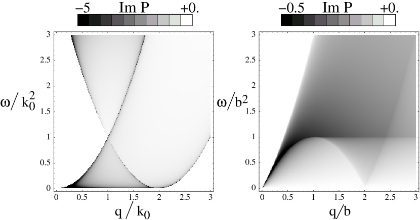
Figure 8: Left hand side: Density plot of the imaginary part of the polarization, $\text{Im}P^{(1),\text{ret}}({\bf q},\omega)/b$, as function of $q$ and $\omega$ in units of $k_{0}$ for $b\to 0$. Right hand side: Density plot of the imaginary part of the susceptibility, $\text{Im}P^{(1),\text{ret}}({\bf q},\omega)$, as function of $q$ and $\omega$ in units of $b\ll k_{0}$.

For $\omega\to 0$, we obtain:

$$\frac{\text{Im}P^{(1),\text{ret}}({\bf q},\omega)}{-(\pi/2bk_{0})}=\left\{\begin{array}[]{l l}\omega^{-1/2}/(q\sqrt{1-(q/2k_{0})^{2}})&;\;0<q<2b\\ 0&;\;q\geq 2b\end{array}\right.$$ (38)

We thus observe a pronounced non-Fermi liquid behavior in the high-energy regime, $b^{2}\leq\omega\leq k_{0}^{2}$. Only in the small energy regime $\omega<b^{2}$, Fermi-liquid behavior is recovered (see next section).

IV.2 Low frequency; forward scattering

In the low-frequency regime, $\omega\sim b^{2}$, we limit ourselves to forward scattering processes with $q\ll 1$. Only considering the lowest order of $\sqrt{\omega}\sim q$, we obtain for $\xi=-1$ the following approximate denominators:

$$D_{1}\to 2q+\gamma 2\sqrt{\omega}e^{-\gamma\varphi}\;,\;D_{2}\to 2q-\gamma 2\sqrt{\omega}e^{-\gamma\varphi}\,,$$

yielding,

Im $$P^{(1),\text{ret},\xi=-1}({\bf q},\omega)$$ (39)

$$\quad\quad=-\frac{1}{2\pi}\int_{-\sinh^{-1}\tilde{b}}^{\text{min}(\ln\tilde{q},\sinh^{-1}\tilde{b})}d\varphi\frac{1}{\sqrt{\tilde{q}^{2}-e^{2\varphi}}}\quad,$$

where we defined $\tilde{b}=b/\sqrt{\omega}$ and $\tilde{q}=q/\sqrt{\omega}$.

For $\xi=1$, and again only considering the lowest order of $\sqrt{\omega}\sim q$, we obtain the following approximate denominators:

$$D_{1}\to 2q-\zeta 2\sqrt{\omega}e^{-\gamma\zeta\varphi}\;,\;D_{2}\to 2q+\zeta 2\sqrt{\omega}e^{-\gamma\zeta\varphi}\,,$$

leading to,

Im $$P^{(1),\text{ret},\xi=1}({\bf q},\omega)$$ (40)

$$\quad\quad=\frac{1}{2\pi}\int_{0}^{\text{min}(\ln\tilde{q},\cosh^{-1}\tilde{b})}d\varphi\frac{1}{\sqrt{\tilde{q}^{2}-e^{2\varphi}}}$$

$$\quad\quad+\frac{1}{2\pi}\int_{\text{max}(-\ln\tilde{q},0)}^{\cosh^{-1}\tilde{b}}d\varphi\frac{1}{\sqrt{\tilde{q}^{2}-e^{-2\varphi}}}\quad.$$

The analytical expressions are presented in appendix B. The behavior for $\omega\to 0$ is given by ($P=-4\pi q\text{Im}P^{(1),\text{ret}}({\bf q},\omega)$):

$$P=\left\{\begin{array}[]{l l}(\omega/b^{2})&;\;0<q<2b\\ (\omega/b^{2})^{1/2}/\sqrt{2}&;q=2b\\ (\omega/b^{2})(1+1/\sqrt{1-(2b/q)^{2}})&;\;q>2b\end{array}\right.$$ (44)

The results are shown on the right hand side of Fig. 8. One sees a linear mode for small wave vectors $q\ll 1$, reminiscent of 1D Luttinger liquids. Nevertheless, the asymptotic behavior of the polarization for small energies shows Fermi-liquid behavior for $q\neq 2b$. At $q=2b$, we find non-Fermi liquid behavior since two parallel regions of the Fermi surface are connected. The non-analyticity at $q=2b$ leads to Friedel oscillations with period $\pi/b$ decaying as $r^{-2}$ at large distances. These results are consistent with alternative analytical treatments for generic Fermi surfaces with arbitrary curvatureGGV97 ; FG02 .

IV.3 Low frequency; backward scattering

For ${\bf q}\approx 2{\bf k}_{0}$, i.e., for backward scattering processes, we consider scattering processes with momentum $2+q$ and $|q|\ll 1$. We then get for $\xi=-1$ the following approximate denominators for low energies $\sqrt{\omega}\sim q$:

$$D_{1}\to\mp 2q+\gamma 2\sqrt{\omega}e^{\gamma\varphi}\quad,\quad D_{2}\to 2\,.$$ (45)

For $\xi=1$, we obtain,

$$D_{1}\to\mp 2q+\zeta 2\sqrt{\omega}e^{\gamma\zeta\varphi}\quad,\quad D_{2}\to 2\;.$$ (46)

The analytical solution is presented in appendix B. Defining $P^{1}+P^{2}=-4\pi\text{Im}P^{(1),\text{ret}}(2{\bf k}_{0}^{\pm},\omega)$ with $|2{\bf k}_{0}^{\pm}|=2+q$, where $q$ can be positive or negative, we obtain the following behavior for $\omega\to 0$:

$$P^{1}=(\omega/b^{2})\left[\frac{1}{2\sqrt{|q|}}+\frac{1}{2\sqrt{2+|q|}}\right]\Theta(-q)\,,$$ (47)

$$P^{2}=\left\{\begin{array}[]{l l}(\omega/b^{2})/2\sqrt{|q|-2b}&;\;q<-2b\\ (\omega/b^{2})^{1/2}/\sqrt{2b}&;\;q=-2b\\ (\omega/b^{2})/2\sqrt{|q|}&;\;-2b<q<0\\ (\omega/b^{2})^{1/2}/\sqrt{2b}&;\;q=0\\ (\omega/b^{2})/2\sqrt{2b-q}&;\;0<q<2b\\ (\omega/b^{2})^{1/2}/\sqrt{2b}&;\;q=2b\\ 0&;\;q>2b\end{array}\right.$$ (55)

The result for “positive” and “negative” back-scattering is shown on the right and left hand side of Fig. 9, respectively.

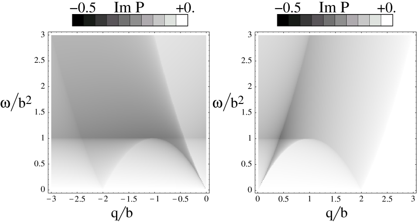
Figure 9: Density plot of the imaginary part of the polarization, $\text{Im}P^{(1),\text{ret}}(2{\bf k}_{0}^{\pm},\omega)$ with $|2{\bf k}_{0}^{\pm}|=2+q$, as function of $q$ and $\omega$ in units of $b\ll k_{0}$.

There are three wave numbers that connect two parallel regions of the Fermi surface and thus lead to non-Fermi liquid behavior. This results in Friedel oscillations with period $\pi/k_{0}$ modulated by oscillations with period $\pi/b$, both decaying as $r^{-2}$ at large distances. These are enhanced by a factor $(2b)^{-1/2}$ compared to the Friedel oscillations originating from forward scattering processes with $q=2b$.

We have integrated Eq. (30) numerically and obtain good agreement between the numerical and the analytical result of appendix B in the whole energy regime and for all wave numbers up to a global factor $0.75$ and $1.3$ in case of forward and backward scattering processes, respectively. In Fig. 10, the numerical (full line) and analytical (dashed line) results for $\text{Im}P^{(1),\text{ret}}$ are shown for $q=3b/2,3b$ (left hand side) and $q=2k_{0}-b/2,2k_{0}-3b$ (right hand side) as function of with $\omega$. In all cases, the low-energy regime is characterized by Fermi-liquid behavior whereas the high-energy shows the square-root divergence predicted by Eq. (38).

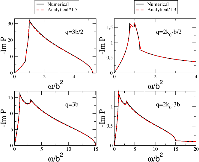
Figure 10: (Color online) The imaginary part of the polarization, $\text{Im}P^{(1),\text{ret}}(q,\omega)$, for $q=3b/2,3b$ (left hand side) and $q=2k_{0}-b/2,2k_{0}-3b$ (right hand side), as function of $\omega$. The solid (black) line shows the numerical and the dashed (red) line the analytical result multiplied by a global factor.

IV.4 The plasmon spectrum

Within the random phase approximation (RPA), the electronic dielectric constant is given by:

$$\epsilon({\bf q},\omega)=1-v_{\bf q}P^{(1),\text{ret}}({\bf q},\omega)\,,$$ (56)

where $v_{\bf q}=2\pi e^{2}/|{\bf q}|$. The plasmon dispersion, $\Omega_{q}$, is then given by the zeros of the dielectric function, $\epsilon({\bf q},\Omega_{q})=0$. In the long wavelength limit, ${\bf q}\to 0$, we have:

$$P^{(1),\text{ret}}({\bf q}\to 0,\omega)=\frac{2q^{2}\alpha n}{\omega^{2}}=\frac{2q^{2}Vv_{F}^{2}n}{\omega^{2}t_{\perp}^{2}}\,.$$ (57)

Let us, at this point, recall the result for a 2D electron gas Stern where the dispersion is given by $E(\bm{k})=k^{2}/(2m^{*})$, where $m^{*}$ is the effective mass. The polarization function is given by:

$$P^{(1),\text{ret}}_{{\rm 2DEG}}({\bf q},\omega) =\frac{nq^{2}}{m^{*}\omega^{2}}\quad,$$ (58)

leading to the well-known result:

$$\Omega_{q}=\left(\frac{2\pi ne^{2}}{m^{*}}q\right)^{1/2}\quad.$$ (59)

Coming back to the Fermi ring and introducing the effective mass $m^{*}=(4\alpha)^{-1}$, we obtain the same expression if we include the degeneracy factor $g_{V}=2$ for the two nonequivalent Fermi points in one graphene layer. With the electrostatic relation $V=e^{2}nd$ ($d$ being the distance between the two layers), we thus obtain

$$\Omega_{q}=\frac{ne^{2}v_{F}}{t_{\perp}}\sqrt{dq}\quad.$$ (60)

V Conclusions

We have analyzed the effect of electron-electron interactions in a biased bilayer graphene in the regime where the Fermi surface has the shape of a ring. We have studied the stability of this system towards ferromagnetic order using a one-band model of the “Mexican hat” dispersion. We find that the spin polarized phase is stable. Unfortunately, our single band calculation does not allow the calculation of the saturation magnetization, which we plan to study in the future, taking into account the full band structure.

The unusual electronic occupation in $k$-space also leads to a deviations from the predictions of Landau’s theory of a Fermi liquid, $\text{Im}P\sim|\omega|$ at low energies, $(Vv_{F}^{2}/t_{\perp}^{2})b^{2}\ll\epsilon\ll(Vv_{F}^{2}/t_{\perp}^{2})k_{0}^{2}$, (see Fig.[10]). The $\text{Im}P\sim|\epsilon|^{-1/2}$ dependence found in this range translates into a quasiparticle lifetime which decays as $\Gamma(\epsilon)\propto\sqrt{|\epsilon-\epsilon_{F}|}$RLTG06 .

At low energies, $\epsilon\ll(Vv_{F}^{2}/t_{\perp}^{2})b^{2}$, the system resembles a Fermi liquid except for wave numbers which connect two parallel regions of the Fermi surface, i.e., for $q=2b,2k_{0}$ and $q=2k_{0}\pm 2b$. Note that, as the Fermi velocity is proportional to the width of the Fermi ring, $b$, the imaginary part of the response function grows as $b^{-2}$. The existence of two Fermi lines implies Friedel oscillations with period $\pi/b$. The plasmon dispersion shows typical features of two-dimensional systems, nevertheless the energy scale is greatly enhanced compared to a 2DEG.

Acknowledgments

This work has been supported by MEC (Spain) through Grant No. FIS2004-06490-C03-00, by the European Union, through contract 12881 (NEST), and the Juan de la Cierva Program (MEC, Spain). N. M. R. Peres thanks the ESF Science Programme INSTANS 2005-2010, and FCT under the grant PTDC/FIS/64404/2006. A. H. C. N was supported through NSF grant DMR-0343790.

Appendix A Coulomb integrals

In this appendix, we list the results for the two relevant Coulomb integrals. The self-energy corrections involve the following Coulomb-integral:

$$I_{1}(a,y) =\int_{0}^{2\pi}\int_{a}^{1}\frac{xdxd\theta}{\sqrt{x^{2}+y^{2}\pm 2xy\cos\theta}}$$ (61)

$$=2(1+y)\bm{E}[g(y)]+2(1-y)\bm{K}[g(y)]$$

$$-2(a+y)\bm{E}[f(y,a)]-2(a-y)\bm{K}[f(y,a)]\,,$$

with $g(y)=4y/(1+y)^{2}$ and $f(y,a)=4ay/(a+y)^{2}$.

The exchange energy gives rise to the following Coulomb-integral:

$$I_{2}(a) =\int_{a}^{1}ydyI_{1}(a,y)=\frac{4}{3(1+a)}\Big{[}2(1+a)(1+a^{3})$$

$$-(1+a)^{2}(1+a^{2})\bm{E}[h(a)]+(1-a^{2})^{2}\bm{K}[h(a)]\,\Big{]}$$ (62)

with $h(a)=4a/(1+a)^{2}$.

Both integrals involve the elliptic integrals $\bm{E}(m)$ and $\bm{K}(m)$ defined as

$$\bm{E}(m)=\int_{0}^{\pi/2}(1-m\sin^{2}\theta)^{1/2}d\theta\,,$$ (63)

and

$$\bm{K}(m)=\int_{0}^{\pi/2}(1-m\sin^{2}\theta)^{-1/2}d\theta\,.$$ (64)

Appendix B Analytical expression for the susceptibility

We will here present the approximate analytical result of the imaginary part for the polarization. For this we define the following abbreviations: $\tilde{q}=q/\sqrt{\omega}$, $\tilde{b}=b/\sqrt{\omega}$, $b_{s}=\tilde{b}+\sqrt{\tilde{b}^{2}+1}$ and $b_{c}=\tilde{b}+\sqrt{\tilde{b}^{2}-1}$ using $\sinh^{-1}x=\ln(x+\sqrt{x^{2}+1})$ and $\cosh^{-1}x=\ln(x+\sqrt{x^{2}-1})$.

B.1 Forward scattering

For the analytic representation of the polarization of forward-scattering processes, we define $f(x)=\cosh^{-1}(\tilde{q}x)$ and abbreviate $P=-2\pi q\text{Im}P^{(1),\text{ret}}({\bf q},\omega)$.
For $0<q<b$, we then have

$$P=\left\{\begin{array}[]{l l}0&;\;\omega>q(2b+q)\\ f(b_{s})&;\;q(2b-q)<\omega<q(2b+q)\\ f(b_{s})-f(b_{c})&;\;0<\omega<q(2b-q)\end{array}\right.$$ (68)

For $b<q<2b$, we have

$$P=\left\{\begin{array}[]{l l}0&;\;\omega>q(2b+q)\\ f(b_{s})&;\;b^{2}<\omega<q(2b+q)\\ f(b_{s})-f(b_{c})+f_{F}(b_{c}^{-1})&;\;q(2b-q)<\omega<b^{2}\\ f(b_{s})-f(b_{c})&;\;0<\omega<q(2b-q)\end{array}\right.$$ (73)

For $q>2b$, we have:

$$P =f(b_{s})\Theta(q(q+2b)-\omega)-f(b_{s}^{-1})\Theta(q(q-2b)-\omega)$$

$$-\left[f(b_{c})-f(b_{c}^{-1})\right]\Theta(b^{2}-\omega)$$

B.2 Backward scattering

For “exact” back-scattering ${\bf q}=2{\bf k}_{0}$, we have with $P=-2\pi\omega^{1/4}\text{Im}P^{(1),\text{ret}}(2{\bf k}_{0},\omega)$ the following expression:

$$P=\sqrt{b_{s}}-\sqrt{b_{s}^{-1}}-\left[\sqrt{b_{s}}-\sqrt{b_{s}^{-1}}\right]$$

For “positive” back-scattering, i.e., ${\bf q}=2{\bf k}_{0}^{+}$ with $|2{\bf k}_{0}^{+}|-2=q>0$, we define $f(x)=\cos^{-1}(\sqrt{\tilde{q}/x})$ and abbreviate $P=-2\pi q^{1/2}\text{Im}P^{(1),\text{ret}}(2{\bf k}_{0}^{+},\omega)$.

For $q<b$, we have:

$$P =f(b_{s})-f(b_{s}^{-1})\Theta(\omega-q(2b+q))$$

$$-\left[f(b_{c})-f(b_{c}^{-1})\Theta(\omega-q(2b-q)\right]\Theta(b^{2}-\omega)$$

For $b<q<2b$, we have:

$$P=\left\{\begin{array}[]{l l}f(b_{s})-f(b_{s}^{-1})&;\;\omega>q(2b+q)\\ f(b_{s})&;\;q(2b-q)<\omega<q(2b+q)\\ f(b_{s})-f(b_{c})&;\;0<\omega<q(2b-q)\end{array}\right.$$ (77)

For $q>2b$, we have:

$$P=\left\{\begin{array}[]{l l}f(b_{s})-f(b_{s}^{-1})&;\;\omega>q(q+2b)\\ f(b_{s})&;\;q(q-2b)<\omega<q(q+2b)\\ 0&;\;0<\omega<q(q-2b)\end{array}\right.$$ (81)

For “negative” back-scattering, i.e., ${\bf q}=2{\bf k}_{0}^{-}$ with $2-|2{\bf k}_{0}^{-}|=q>0$, we define $f_{s}(x)=\sinh^{-1}(\sqrt{\tilde{q}x})$ and $f_{c}(x)=\cosh^{-1}(\sqrt{\tilde{q}x})$. The polarization is given by $P^{1}+P^{2}=-2\pi q^{1/2}\text{Im}P^{(1),\text{ret}}(2{\bf k}_{0}^{-})$. The first part is independent of the relative value of $q$ and $\omega$ and reads

$$P^{1} =f_{s}(b_{s})-f_{s}(b_{s}^{-1})-\left[f_{s}(b_{c})-f_{s}(b_{c}^{-1})\right]\Theta(b^{2}-\omega)\;.$$

For $0<q<b$, we further have:

$$P^{2}=\left\{\begin{array}[]{l l}0&;\;\omega>q(2b+q)\\ f_{c}(b_{s})&;\;q(2b-q)<\omega<q(2b+q)\\ f_{c}(b_{s})-f_{c}(b_{c})&;\;0<\omega<q(2b-q)\end{array}\right.$$ (85)

For $a<q<2b$, we have:

$$P^{2}=\left\{\begin{array}[]{l l}0&;\;\omega>q(2b+q)\\ f_{c}(b_{s})&;\;b^{2}<\omega<q(2b+q)\\ f_{c}(b_{s})-f_{c}(b_{c})+f_{c}(b_{c}^{-1})&;\;q(2b-q)<\omega<b^{2}\\ f_{c}(b_{s})-f_{c}(b_{c})&;\;0<\omega<q(2b-q)\end{array}\right.$$ (90)

For $q>2b$, we have:

$$P^{2} =f_{c}(b_{s})\Theta(q(q+2b)-\omega)-f_{c}(b_{s}^{-1})\Theta(q(q-2b)-\omega)$$

$$-\left[f_{F}(b_{c})-f_{F}(b_{c}^{-1})\right]\Theta(b^{2}-\omega)$$

References

- (1) K. S. Novoselov, A. K. Geim, S. V. Morozov, D. Jiang, Y. Zhang, S. V. Dubonos, I. V. Grigorieva, and A. A. Firsov, Science 306, 666 (2004).
- (2) N. M. R. Peres, F. Guinea, and A. H. Castro Neto, Phys. Rev. B 73, 125411 (2006).
- (3) E. McCann and V. I. Fal’ko, Phys. Rev. Lett. 96, 086805 (2006).
- (4) E. McCann, Phys. Rev. B 74, 161403(R) (2006).
- (5) F. Guinea, A. H. Castro Neto, and N. M. R. Peres, Phys. Rev. B 73, 245426 (2006), and unpublished results.
- (6) Eduardo V. Castro, K. S. Novoselov, S. V. Morozov, N. M. R. Peres, J. M. B. Lopes dos Santos, Johan Nilsson, F. Guinea, A. K. Geim, and A. H. Castro Neto, cond-mat/0611342.
- (7) T. Ohta, A. Bostwick, T. Seyller, K. Horn, and E. Rotenberg, Science 312, 951 (2006);
- (8) C. Berger, Z. M. Song, T. B. Li, X. B. Li, A. Y. Ogbazghi, R. Feng, Z. T. Dai, A. N. Marchenkov, E. H. Conrad, P. N. First, and W. A. de Heer, J. Phys. Chem. B, 108, 19912 (2004).
- (9) K. S. Novoselov, A. K. Geim, S. V. Morozov, D. Jiang, M. I. Katsnelson, I. V. Grigorieva, S. V. Dubonos, and A. A. Firsov, Nature 438, 197 (2005); Y. Zhang, Y.-W. Tan, H. L. Stormer, and P. Kim, Nature 438, 201 (2005).
- (10) Y. Zhang, Z. Jiang, J. P. Small, M. S. Purewal, Y. W. Tan, M. Fazlollahi, J. D. Chudow, J. A. Jaszczak, H. L. Stormer, and P. Kim, Phys. Rev. Lett. 96, 136806 (2006).
- (11) K. Nomura and A. H. MacDonald, Phys. Rev. Lett. 96, 256602 (2006); Jason Alicea and Matthew P. A. Fisher, Phys. Rev. B 74, 075422 (2006); Kun Yang, S. Das Sarma, and A. H. MacDonald, Phys. Rev. B 74, 075423 (2006); M. O. Goerbig, R. Moessner, and B. Doucot, Phys. Rev. B 74, 161407(R) (2006); V. P. Gusynin, V. A. Miransky, S. G. Sharapov, I. A. Shovkovy, Phys. Rev. B 74, 195429 (2006).
- (12) I. F. Herbut, Phys. Rev. Lett. 97, 146401 (2006).
- (13) E. G. Mishchenko, cond-mat/0612651.
- (14) O. Vafek, Phys. Rev. Lett. 97, 266406 (2006); E. H. Hwang, S. Das Sarma, cond-mat/0610561; B. Wunsch, T. Stauber, F. Sols, and F. Guinea, New J. Phys. 8, 318 (2006).
- (15) J. González, F. Guinea, and M. A. H. Vozmediano, Phys. Rev. Lett. 77, 3589 (1996).
- (16) Strictly speaking, marginal Fermi liquid behavior, as defined in the context of high temperature superconductors varma , applies to systems with parabolic dispersion and a continuous Fermi surface. In that case, quasiparticles are not well defined because their spectral function is as broad as their energy. Graphene, on the other hand, has linearly dispersing electrons, that is, Dirac fermions, and a Fermi surface consisting of points at the edge of the Brillouin zone. Hence, the concept of a marginal Fermi liquid is dull in their context.
- (17) C. M. Varma, P. B. Littlewood, S. Schmitt-Rink, E. Abrahams, and A. E. Ruckenstein, Phys. Rev. Lett. 63, 1996 (1989).
- (18) N. M. R. Peres, F. Guinea, and A. H. Castro Neto, Phys. Rev. B 72, 174406 (2005).
- (19) T. Stauber, F. Guinea, and M.A.H. Vozmediano, Phys. Rev. B 71, 041406(R) (2005); D. V. Khveshchenko, Phys. Rev. B 74, 161402(R) (2006).
- (20) X. F. Wang and T. Chakraborty, Phys. Rev. B 75, 041404(R) (2007).
- (21) J. W. McClure, Phys. Rev. 108, 612 (1957).
- (22) F. Stern, Phys. Rev. Lett. 18, 546 (1967).
- (23) J. González, F. Guinea, and M.A.H. Vozmediano, Phys. Rev. Lett. 79, 3514 (1997).
- (24) S. Fratini and F. Guinea, Phys. Rev. B 66, 125104 (2002).
- (25) R. Roldán, M. P. López-Sancho, S.-W. Tsai, and F. Guinea, Europhys. Lett. 76, 1165 (2006).