Mean field theory and fluctuation spectrum of a pumped, decaying Bose-Fermi system across the quantum condensation transition

Abstract

We study the mean-field theory, and the properties of fluctuations, in an out of equilibrium Bose-Fermi system, across the transition to a quantum condensed phase. The system is driven out of equilibrium by coupling to multiple baths, which are not in equilibrium with each other, and thus drive a flux of particles through the system. We derive the self-consistency condition for an uniform condensed steady state. This condition can be compared both to the laser rate equation and to the Gross-Pitaevskii equation of an equilibrium condensate. We study fluctuations about the steady state, and discuss how the multiple baths interact to set the system’s distribution function. In the condensed system, there is a soft phase (Bogoliubov, Goldstone) mode, diffusive at small momenta due to the presence of pump and decay, and we discuss how one may determine the field-field correlation functions properly including such soft phase modes. In the infinite system, the correlation functions differ both from the laser and from an equilibrium condensate; we discuss how in a finite system, the laser limit may be recovered.

I Introduction

In the last decade there have been enormous advances in the experimental realisation and theoretical understanding of the phenomenon of quantum condensation, i.e macroscopic occupation of a single quantum mode, in different physical conditions. The phenomena ranges from Bose-Einstein Condensation (BEC) of structureless bosons to the BCS-type collective state of fermions and has been studied in several physical systems such as degenerate atomic gases and superconductors SnokeBook . Further, recent experimental advances in manipulation of atomic Fermi gases have led to realisation of the BCS-BEC crossover regime Regal04 ; Zweierlein04 and low-dimensional atomic condensates have also been exploredGorlitz01 ; Paredes04 ; Kinoshita04 ; Stock05 . From the early days of experimental investigation of BEC there have been enormous efforts in order to realise quantum condensation in the solid state SnokeBook . For this, the currently promising candidates are excitons in coupled quantum wells Butov02a ; Butov02b ; Snoke02 , microcavity polaritons Dang98 ; Deng ; Richard , quantum Hall bilayers QH , and Josephson junction arrays in microwave cavities JJ . Although all these systems potentially may condense at temperatures orders of magnitude higher than those for dilute atomic gases, it has proven to be much more difficult to realise BEC in the solid state than in atomic traps. Recently a comprehensive set of experiments Kasprzak06 reports polariton condensation in CdTe based microcavities but still the level of control in the study of the condensed states in solid-state is far from the finesse achieved in atomic vapours.

In these various candidates for condensation, one should distinguish different classes of systems. Equilibrium superconductors are special in that the decay of pairs is disallowed. In equilibrium particle-hole condensates, such as quantum Hall bilayers or charge density waves, particle-hole mixing (tunnelling in bilayers) leads to a gapped spectrum; however the gap may be very small. Non-equilibrium particle-hole condensates in the solid state are, to a much greater extent than atomic gases, subject to dephasing and decay. It is not usually possible to isolate the condensate from the environment: lattice phonons, impurities and imperfections of the crystal structure lead to dephasing, and due to poor trapping, particles escape, requiring external pumping to sustain a steady-state. The dephasing and decay processes are often faster than thermalisation, putting the system out of thermal equilibrium. The decay, and consequent lack of equilibrium have for a long time presented the major experimental obstacle in the realisation of solid-state condensation in otherwise appropriate conditions. Even if one can accelerate thermalisationKasprzak06 ; Hui06 , comparing the decay rates to other energy scales, one may see that decay, and the consequent flux of particles through the system, remains a more important effect in solid state than in atomic gases.

Thus, a significant presence of dissipation and decay also poses fundamental questions about the robustness of a condensate, for example: whether a steady-state condensate is possible with incoherent pumping and decay, and if so, how does it differ from thermal equilibrium, and from a laserkeldysh_letter . Quantum condensation in dissipative systems also provides a connection to other phenomena of collective behaviour in the presence of dissipation such as pattern formationCrossHohenberg ; Haken:RMP , particularly in lasersHaken70 ; Staliunas ; Denz03 , and also recently in a system related to that studied here, the coherently pumped polariton optical parametric oscillatorWouters05 ; Wouters06 . Other recent examples of phase transitions and coherence in driven systems include quantum criticality in magnetic systems in the presence of currentsMitra ; Hogan , and transport through a Kondo dot coupled to multiple dotsPaaske . The relation between lasing and BEC is particularly relevant for polariton BEC, where the experimental distinction between the two is not straightforward Szymanska .

Microcavity polaritons in particular, being made from fermionic particles and photons, have several special features and so provide an excellent laboratory to study condensation in dissipative environment. Due to the large wave-length of their photonic component and non-linearities associated with underlying fermionic structure the physics exits the regime of weakly interacting bosons at even modest density Keeling . Putting aside a few subtleties characteristic only for polaritons one can say that with increasing density the quantum condensation transition moves from BEC (fluctuation dominated) to something like the BCS (mean-field, interaction dominated) collective state Keeling , analogous to the BCS-BEC crossover in atomic Fermi gases near Feshbach resonance Regal04 ; Zweierlein04 . This allows one to explore the influence of non-equilibrium and dissipation not only on the usual BEC but also on more exotic forms of quantum condensation. A further complication is that polaritons in planar microcavities are two-dimensional(2D) particles and so in an infinite equilibrium system, although there is a Berezhinskii-Kosterlitz-Thouless (BKT) transition to a superfluid phase, below the transition long-wavelength fluctuations destroy the off-diagonal long range order and result in algebraic decay of phase coherence. Dissipation changes the structure of collective modes and influences the spatial and temporal coherence in 2D quasicondensates, changing the power-law controlling the decay of phase correlations keldysh_letter . Finally, microcavity polaritons can also be trapped either in stress-induced harmonic potentialsSnoke06 ; Daif06 ; Baas06 or in natural traps provided by microcavity disorder which reduce the influence of long-wavelength fluctuations and may allow the existence of a true condensate and phase coherence over the whole system size Kasprzak06 . How this confinement, when combined with pumping and decay, modifies the properties of coherence in such systems is an interesting questionsavaona06 , which has not yet been fully addressed.

The last issue is particularly relevant for the deeper understanding of the differences and connections between a polariton condensate and the laser. Apart from the obvious difference; the laser being a collective coherent state of massless non-interacting photons while the condensate consists of massive and interacting bosons (in polariton condensation both massive photons and strongly coupled excitons are coherent), there are more subtle differences connected with fluctuations and so expected differences in the decay of correlations keldysh_letter . Lasing is normally considered in systems with a well-defined single or a few mode structure and so the phase fluctuations which control the laser linewidth are those of a phase diffusion of a single modeHaken:Laser . In contrast, condensation is usually studied in systems where there is a continuum of single particle modes, and thus collective excitations involve coherent interaction of these different modes which affects the decay of coherence and the line-shape of the emission keldysh_letter . While lasing in systems with transverse freedom has been investigated for its pattern forming propertiesDenz03 , there remain many open questions concerning the decay of correlations and the crossover from a small system with few spatial modes to the infinite and many-mode limit.

Although semiconductor microcavities in strong coupling provide a natural system to explore such phenomena, all these issues are by no means restricted to polariton condensation. With recent advances in manipulating dilute atomic gases similar conditions can be engineered, an immediate example is that of an atom laser in which a continuous leakage of atoms from atomic BEC takes place. To our knowledge the description of the output from an atom laser has been to date largely analogous to that of the photon laserHolland96 and the influence of the continuum of modes connected with atomic BEC on the coherence properties of the atom laser has not been addressed.

In a previous paperkeldysh_letter we addressed some of these issues. We used a model Bose-Fermi system coupled to independent baths, not in thermal or chemical equilibria with each other, providing incoherent pumping and decay. We show that steady-state spontaneous condensation can occur in such systems, and can be distinct from lasing: The condensate can exist at low densities, far from the inversion required for lasing. We also found that the collective modes are qualitatively altered by the presence of pumping and decay: The low energy phase mode (Goldstone, Bogoliubov mode) becomes diffusive at small momenta. By considering the effect of phase fluctuations, we described the decay of correlations, which at large times and distances differs both from that for a thermal equilibrium condensate and from a laser.

In this manuscript, apart from providing technical details of the method we address several new aspects of quantum condensation in dissipative environment. In particular we study the influence of the exciton density of states, and the temperature of the pumping bath on the non-equilibrium phase diagram. We also analyse how the non-thermal occupation of photon states is controlled by competition between the pumping and decay baths, and how this occupation deviates from that in thermal equilibrium. We do not a priori assume that the system is close to equilibrium, and so the system’s distribution function may be of any form. Finally we provide a full account of how to determine field-field correlation functions in the condensed state, where phase fluctuations may be large, and so expansion to second order is insufficient. These field-field correlation functions describe the decay of correlations at large times and distances, and their Fourier transform gives the line-shape of a non-equilibrium condensate. This is an important extension to the non-equilibrium path integral techniques which to our knowledge has not been done before. In the final section of this paper we study how dissipation influences spatial and temporal coherence in a finite size condensate and show how the linewidth of emission from polariton or atom condensate should be determined taking proper account of the spatial fluctuations. We further emphasise the fundamental difference between emission from a polariton condensate or an atom laser and that from the photon laser.

The paper is organised as follows: The model for the system, and for the reservoirs to which it is coupled is introduced in Sec. II, then in Sec. III we show how to integrate out first the reservoirs, and then the fermionic fields to give an effective action in terms of the photon field. We then study this effective action in the saddle-point approximation in Sec. IV. In Sec. V, by discussing fluctuations about the saddle point we consider the stability of the saddle-point solutions, and show how the instability of the normal state, and the photon distribution functions, compare to an equilibrium treatment. Having identified the stable and unstable saddle-point solutions, Sec. VI then presents numerical results for the critical conditions at which steady-state, non-equilibrium condensation occurs. The effects of fluctuations on correlation functions in the condensed case are studied again in Sec. VII, where care is taken to correctly describe phase fluctuations in the broken symmetry system. Section VIII then studies how finite size modifies correlation functions, and the relation between the previous results and laser theory. Finally, section IX summarises our results.

II Model

Our Hamiltonian is

$$\hat{H}=\hat{H}_{\rm{sys}}+\hat{H}_{\rm{sys,bath}}+\hat{H}_{\rm{bath}},$$ (1)

where,

$$\hat{H}_{\rm{sys}}=\sum_{\alpha}\epsilon_{\alpha}\left(b_{\alpha}^{\dagger}b_{\alpha}-a_{\alpha}^{{\dagger}}a_{\alpha}\right)+\sum_{{\mathbf{p}}}\omega_{{\mathbf{p}}}\psi_{{\mathbf{p}}}^{\dagger}\psi_{{\mathbf{p}}}\\ +\displaystyle\frac{1}{\sqrt{L^{2}}}\sum_{\alpha}\sum_{{\mathbf{p}}}\left(g_{\alpha,{\mathbf{p}}}\psi_{{\mathbf{p}}}b_{\alpha}^{\dagger}a_{\alpha}+\text{H.c.}\right)$$ (2)

describes two fermionic species $b_{\alpha}$ and $a_{\alpha}$, interacting with bosonic modes $\psi_{{\mathbf{p}}}$ normalised in a 2D box of area $L^{2}$, with $L\to\infty$. Condensed solutions of Eq. (2) have been studied in the context of atomic Fermi gases Holland01 ; Timmermanns01 ; Ohashi02 and microcavity polaritons Eastham ; Keeling ; Marchetti . In this work we focus on microcavity polaritons, and so this model describes the interaction between disorder-localised excitons which are dipole coupled to cavity photon modes $\psi_{{\mathbf{p}}}$, with low ${\mathbf{p}}$ dispersion, $\omega_{{\mathbf{p}}}\simeq\omega_{0}+{\mathbf{p}^{2}}/2m_{\text{ph}}$, where $m_{\text{ph}}=(\hbar/c)(2\pi/w)$ is the photon mass in a 2D microcavity of width $w$. The disorder localised excitons are described here as in previous works Eastham ; Keeling ; Marchetti by hard-core bosons; i.e. the Coulomb interaction between excitons is described by exclusion, preventing multiple occupation of a single disorder-localised state $\alpha$. This hard core boson is represented by a two-level system, described here as two fermionic levels, $b^{\dagger}_{\alpha},a_{\alpha}$. Thus, the combination $b^{\dagger}_{\alpha}a_{\alpha}$ creates an exciton in the localised state with energy $\epsilon_{\alpha}$. This energy $\epsilon_{\alpha}$ includes the Coulomb binding within an exciton state. In such a description, it is important not to confuse the fermion states (representing a hard-core bound exciton) with the underlying conduction and valence band states (see e.g. Refs. SST, ; Marchetti, for further discussion of this point). In order that these fermionic levels describe a two-level system, it is necessary that the constraint $b^{\dagger}_{\alpha}b_{\alpha}+a^{\dagger}_{\alpha}a_{\alpha}=1$ is satsified; i.e. that exactly one of the two levels is occupied. In thermal equilibrium, this constraint can be exactly imposed by a shift of Matsubara frequenciesPopov88 ; and in that case it can be easily seen that the difference between imposing the single occupancy constraint exactly and imposing it on average leads only to a factor of 2 in the definition of temperature. Out of thermal equilibrium, no simple shift to the Matsubara frequencies is possible, although an extension to the non-equilibrium case has been proposedKiselev00 . For simplicity, in this work, we will impose the single occupancy constraint on average, as discussed below when introducing the occupation functions of the bath.

Because of the imperfect reflectivity of the cavity mirrors, photons escape, so the system must be pumped (excitons injected) to sustain a steady-state. As illustrated schematically in Fig. 1, the imperfect reflectivity of the mirrors is represented by coupling to the continuum of bulk photon modes.

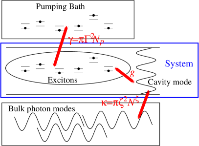
Figure 1: (Color online) Schematic diagram illustrating parts of the Fermi-Bose system, and its coupling to baths. The parts in the box labelled system are described by Eq. (2), while the effective couplings to the baths, described by Eq. (3), lead to effective pump and decay rates $\gamma$ and $\kappa$ as discussed later.

Incoherent fermionic pumping is described by coupling to a pumping bath — which is represented mathematically as two separate fermionic baths, coupled to the two fermionic modes. Thus, the coupling of the system to these pumping and decay baths is written as:

$$\hat{H}_{\rm{sys,bath}}=\sum_{\alpha,k}\Gamma^{a}_{\alpha,k}(a^{\dagger}_{\alpha}A_{k}+\text{H.c.})+\Gamma^{b}_{\alpha,k}(b^{\dagger}_{\alpha}B_{k}+\text{H.c.})\\ +\sum_{{\mathbf{p}},k}\zeta_{{\mathbf{p}},k}(\psi_{{\mathbf{p}}}^{\dagger}\Psi_{k}+\text{H.c.}),$$ (3)

Here $A_{k},B_{k}$ are fermionic annihilation operators for the pump baths, while $\Psi_{k}$ are bosonic annihilation operators for photon modes outside the cavity. The Hamiltonian corresponding to the evolution of these baths is given by:

$$\hat{H}_{\rm{bath}}=\sum_{k}\omega^{\Gamma^{a}}_{k}A_{k}^{\dagger}A_{k}+\sum_{k}\omega^{\Gamma^{b}}_{k}B_{k}^{\dagger}B_{k}+\sum_{k}\omega^{\zeta}_{k}\Psi_{k}^{\dagger}\Psi_{k}.$$ (4)

The pumping bath, if thermalised at some finite non-zero temperature, acts both as a source of particles, and also tries to drive the polariton distribution function towards a thermal distribution in equilibrium with the bath. In some physical systems, one might also consider a bath which purely provides a thermalisation mechanism, such as phonons, which redistribute energy, but do not change particle number. We do not explicitly consider such a bath. However, in the example of microcavity polaritons, our model may still capture much of the important behaviour, for the following reason. One may consider the low energy polaritons as being pumped by a reservoir of higher energy excitons. These excitons are formed by the binding of the electrons and holes injected by the pump laser, and subsequent relaxation by phonon emission, and are thus partially thermalised. By regarding our pumping bath as describing a partially thermalised exciton reservoir, our model, being interacting, could thus describe the thermalisation of low energy polaritons pumped by such a reservoir.

Although in the absence of other processes, the excitons would thermalise to the pumping bath, they are also strongly coupled to photons, which in turn couple to a second environment of the bulk photon modes outside the cavity. The strongly coupled exciton-photon system would be therefore influenced by two independent environments which are not in thermal or chemical equilibrium with each other. Even in the steady-state, if the rates of dissipation to the environment are larger than the polariton-polariton interactions, the system would remain out of thermal equilibrium. In addition, even if the thermalisation via polariton-polariton interaction is fast, so the system distribution function would be close to thermal, particles are continuously added and removed from the system. We show that this particle “current” has dramatic consequences on the properties of such a condensate even if it remains close to equilibrium.

We would like to stress that there are two distinct issues, both of which we intend to address. The first is that of non-equilibrium distribution functions, in systems where the internal thermalisation rate is slower than the pumping and decay rates — i.e. when the coupling to the external baths is strong, and the baths are not in equilibrium with each other. The second issue is the presence of particle “current” in strongly dissipative systems — even if internal thermalisation rates are large, this current may be important if the pumping, decay and thermalisation rates are large compared to other energy scales.

In the next section we will introduce the path integral formalism which will allow us to treat the nonequilibrium conditions. Our approach will then be to assume that the pumping and decay baths are much larger than the system, and so the populations in the baths are fixed. This will enable us to describe the properties of the system as influenced by its coupling to the baths. These influences modify both the system’s spectrum and the population of this spectrum. We will look for steady states of the system in the presence of pumping and decay, and study the excitation spectra around these steady states.

III Path Integral Formulation

In order to study the system away from thermal equilibrium, we proceed using the path-integral formulation of non-equilibrium Keldysh field theory, as described in detail in Ref. Kamenev, . Following the prescription there, we write the quantum partition function as a coherent state path integral over bosonic and fermionic fields defined on a closed-time-path contour, $\mathcal{C}$. Arranging the fermionic fields into a Nambu vector $\bar{\phi}=(\bar{b},\bar{a})$ and $\phi=(b,a)^{\rm T}$, loosely referred to as “particle/hole” space, the partition function can be formally written as:

$${\cal Z}={\cal N}\int\prod_{{\mathbf{p}}}D[\bar{\psi}_{{\mathbf{p}}},\psi_{{\mathbf{p}}}]\prod_{\alpha}D[\bar{\phi}_{\alpha},\phi_{\alpha}]\\ \times\prod_{k}D[\bar{A}_{k},A_{k},\bar{B}_{k},B_{k},\bar{\Psi}_{k},\Psi_{k}]e^{iS},$$

where ${\cal N}$ represents a constant of normalisation and the total action can be separated into constituent components $S=S_{\phi}+S_{\psi}+S_{{\rm bath},\phi}+S_{{\rm bath},\psi}$. The part:

$$S_{\phi}=\int\limits_{\cal C}dt\sum_{\alpha,{\mathbf{p}}}\bar{\phi}_{\alpha}\left[i\partial_{t}-\epsilon_{\alpha}\sigma_{3}-g_{\alpha,{\mathbf{p}}}\bar{\psi}_{\mathbf{p}}\sigma_{-}-g_{\alpha,{\mathbf{p}}}\psi_{\mathbf{p}}\sigma_{+}\right]\phi_{\alpha},$$

describes the free exciton evolution together with the dipole interaction between excitons and photons. Due to the Nambu formalism, the term in brackets is a matrix, and has been decomposed in terms of the Pauli matrices $\sigma_{i}$ operating in the particle-hole $(b,a)$ space (with $\sigma_{0}=1$). The time derivative is taken along the Keldysh contour ${\cal C}$. Similarly,

$$S_{\psi}=\int\limits_{\cal C}dt\;\sum_{{\mathbf{p}}}\bar{\psi}_{\mathbf{p}}\left(i\partial_{t}-\omega_{{\mathbf{p}}}\right)\psi_{{\mathbf{p}}}$$

describes the free photon dynamics. The excitonic environment and the interactions between excitons and their environment is given by

$$S_{{\rm bath},\phi}=\int\limits_{\cal C}dt\sum_{\alpha,k}[\bar{A}_{k}\left(i\partial_{t}-\omega^{\Gamma^{a}}_{k}\right)A_{k}+\bar{B}_{k}\left(i\partial_{t}-\omega^{\Gamma^{b}}_{k}\right)B_{k}$$

$$-\Gamma^{b}_{\alpha,k}(\bar{b}_{\alpha}B_{k}+\bar{B}_{k}b_{\alpha})-\Gamma^{a}_{\alpha,k}(\bar{a}_{\alpha}A_{k}+\bar{A}_{k}a_{\alpha})],$$

while the photonic environment is given by

$$S_{{\rm bath},\psi}=\int\limits_{\cal C}dt\sum_{{\mathbf{p}},k}[\bar{\Psi}_{k}\left(i\partial_{t}-\omega^{\zeta}_{k}\right)\Psi_{k}-\\ \zeta_{{\mathbf{p}},k}\left(\bar{\psi}_{\mathbf{p}}\Psi_{k}+\bar{\Psi}_{k}\psi_{\mathbf{p}}\right)].$$

As described in Ref. Kamenev, , the standard procedure is to replace the fields on the closed-time-path contour by a doublet of fields $\psi=(\psi_{f},\psi_{b})$ on the forward and backward branches. This then leads to four Green’s functions: forward $iG^{<}(t,t^{\prime})=\langle\psi_{f}(t)\psi^{\dagger}_{b}(t^{\prime})\rangle$, backward $iG^{>}(t,t^{\prime})=\langle\psi_{b}(t)\psi^{\dagger}_{f}(t^{\prime})\rangle$, time-ordered $iG^{T}(t,t^{\prime})=\langle\psi_{f}(t)\psi^{\dagger}_{f}(t^{\prime})\rangle$, and anti-time-ordered $iG^{\tilde{T}}(t,t^{\prime})=\langle\psi_{b}(t)\psi^{\dagger}_{b}(t^{\prime})\rangle$. In the homogeneous steady-state these are functions of $r-r^{\prime}$ and $t-t^{\prime}$ alone and when transformed into ${\mathbf{p}}$ and $\omega$ space, in the case of photon fields, the functions $iG^{<}$ and $iG^{>}$ give the luminescence and absorption spectra respectively. Again following Ref. Kamenev, , as these four Green’s functions are not independent, one proceeds by making a rotation to classical $\phi_{cl}=(\phi_{f}+\phi_{b})/\sqrt{2}$ and quantum $\phi_{q}=(\phi_{f}-\phi_{b})/\sqrt{2}$ components. All fields are from now vectors in Keldysh space, i.e $\psi=(\psi_{cl},\psi_{q})$, and we define an additional matrix in Keldysh $(cl,q)$ space:

$$\psi^{M}={\frac{1}{\sqrt{2}}}\left(\begin{array}[]{cc}\psi_{cl}&\psi_{q}\\ \psi_{q}&\psi_{cl}\end{array}\right)=\psi_{cl}\sigma_{0}^{K}+\psi_{q}\sigma_{1}^{K},$$

(where $\sigma_{i}^{K}$ are Pauli matrices in Keldysh space). One may then write the action as:

$$S_{\phi}=\int_{-\infty}^{\infty}dt\sum_{\alpha,{\mathbf{p}}}\\ \bar{\phi}_{\alpha}[i\partial_{t}-\epsilon_{\alpha}\sigma_{3}-\frac{g_{\alpha,{\mathbf{p}}}}{\sqrt{2}}\bar{\psi}_{\mathbf{p}}^{M}\sigma_{-}-\frac{g_{\alpha,{\mathbf{p}}}}{\sqrt{2}}\psi_{\mathbf{p}}^{M}\sigma_{+}]\sigma_{1}^{\textsc{k}}\phi_{\alpha},$$

$$\begin{aligned} S_{\psi}=\int_{-\infty}^{\infty}dt\;\sum_{\mathbf{p}}\bar{\psi}_{\mathbf{p}}\left(i\partial_{t}-\omega_{\mathbf{p}}\right)\sigma_{1}^{\textsc{k}}\psi_{\mathbf{p}},\end{aligned}$$

$$S_{{\rm bath}\phi}=\int_{-\infty}^{\infty}dt\sum_{\alpha,k}[-\Gamma^{b}_{\alpha,k}(\bar{b}_{\alpha}\sigma_{1}^{\textsc{k}}B_{k}+\bar{B}_{k}\sigma_{1}^{\textsc{k}}b_{\alpha})\\ -\Gamma^{a}_{\alpha,k}(\bar{a}_{\alpha}\sigma_{1}^{\textsc{k}}A_{k}+\bar{A}_{k}\sigma_{1}^{\textsc{k}}a_{\alpha})\\ +\bar{B}_{k}\left(i\partial_{t}-\omega^{\Gamma^{b}}_{k}\right)\sigma_{1}^{\textsc{k}}B_{k}+\bar{A}_{k}\left(i\partial_{t}-\omega^{\Gamma^{a}}_{k}\right)\sigma_{1}^{\textsc{k}}A_{k}],$$

$$S_{{\rm bath}\psi}=\int_{-\infty}^{\infty}dt\sum_{{\mathbf{p}},k}[-\zeta_{{\mathbf{p}},k}\left(\bar{\psi}_{\mathbf{p}}\sigma_{1}^{\textsc{k}}\Psi_{k}+\bar{\Psi}_{k}\sigma_{1}^{\textsc{k}}\psi_{\mathbf{p}}\right)\\ +\bar{\Psi}_{k}\left(i\partial_{t}-\omega^{\zeta}_{k}\right)\sigma_{1}^{\textsc{k}}\Psi_{k}].$$

III.1 Treatment of environment

As we are interested in the properties of the system, rather than the properties of the baths, we next integrate over the bath fields, to leave an effective action expressed only in terms of the fields describing the system. If the baths are much larger than the system, then their behaviour is not affected by the interaction with the system. One may then evaluate correlation functions of bath operators as for free bosons and free fermions; these correlators in turn depend on the distribution function of the baths, i.e. the population of the bath modes. The effects of the environment then enter as self energies for the system fields, which modify both the spectrum and its occupation. This procedure is described in Ref. Kamenev, ; we summarise the results here both to show how it applies to our system, and also as our notation differs slightly from Ref. Kamenev, For the decay (photon) bath one has:

$$S_{{\rm bath}\psi}=-\int\int_{-\infty}^{\infty}dtdt^{\prime}\sum_{{\mathbf{p}},{\mathbf{p}^{\prime}}}\\ \bar{\psi}_{\mathbf{p}}(t)\sigma_{1}^{\textsc{k}}\sum_{k}\zeta_{{\mathbf{p}},k}\zeta_{{\mathbf{p}^{\prime}},k}\left[(i\partial_{t}-\omega^{\zeta}_{k})\sigma_{1}^{\textsc{k}}\right]^{-1}\sigma_{1}^{\textsc{k}}\psi_{{\mathbf{p}^{\prime}}}(t^{\prime}),$$

In Keldysh space the Green’s function for a free boson has the following form

$$\left[(i\partial_{t}-\omega^{\zeta}_{k})\sigma_{1}^{\textsc{k}}\right]^{-1}=\left(\begin{array}[]{cc}\hat{D}_{k}^{K}(t-t^{\prime})&\hat{D}_{k}^{R}(t-t^{\prime})\\ \hat{D}_{k}^{A}(t-t^{\prime})&0\end{array}\right),$$

where (after the Fourier transform with respect to $t-t^{\prime}$) the retarded, advanced and Keldysh Green’s functions are respectively

$$\hat{D}_{k}^{R/A}(\omega)= \frac{1}{\omega-\omega^{\zeta}_{k}\pm i0},$$

$$\hat{D}_{k}^{K}(\omega)= (-2\pi i)(2n_{B}(\omega^{\zeta}_{k})+1)\delta(\omega-\omega^{\zeta}_{k}).$$

If the bath distributions are thermal, then $n_{B}$ would be the Bose occupation functions, however one can also consider arbitrary function for $n_{B}$.

Let us now make a number of restrictions on the photon bath, to simplify the analysis. Firstly, we will assume that $S_{\text{bath}\psi}$ does not contain terms off-diagonal in ${\mathbf{p}}{\mathbf{p}^{\prime}}$. This means that each confined photon mode ${\mathbf{p}}$ couples to a separate set of bulk photon modes, i.e. that $\zeta_{{\mathbf{p}},k}\zeta_{{\mathbf{p}^{\prime}},k}=0$ unless ${\mathbf{p}}={\mathbf{p}^{\prime}}$. Physically, this can be interpreted as conservation of in-plane momentum in the coupling of two-dimensional microcavity photon modes to bulk modes. Next, we restrict to the case that all ${\mathbf{p}}$ photonic modes couple to their environments with the same strength i.e $\zeta_{{\mathbf{p}},k}=\zeta_{k}$. Then, if the bath frequencies $\omega^{\zeta}_{k}$ form a dense spectrum, and the coupling constants $\zeta_{k}$ are smooth functions of the frequencies, we may replace the sum over bath modes by an integral,

$$\sum_{k}\zeta_{k}^{2}\to\int d\omega^{\zeta}\zeta(\omega^{\zeta})^{2}N^{\zeta}(\omega^{\zeta}),$$

where we have introduced $N^{\zeta}(\omega^{\zeta})$ as the bath’s density of states. After integrating over $\omega^{\zeta}$ we obtain

$$S_{{\rm bath}\psi}=-\int_{-\infty}^{\infty}d\omega\sum_{{\mathbf{p}}}\bar{\psi}_{\mathbf{p}}(\omega)\left(\begin{array}[]{cc}0&d^{A}\\ d^{R}&d^{K}\end{array}\right)_{(-\omega)}\psi_{\mathbf{p}}(-\omega).$$

By writing $d^{R,A}(\omega)=R(\omega)\mp i\kappa(\omega)$ we may split the bath self energy into an imaginary part, describing broadening

$$\kappa(\omega)=\pi\zeta^{2}(\omega)N^{\zeta}(\omega),$$

and a real energy shift,

$$R(\omega)=\int d\omega^{\zeta}\frac{\zeta^{2}(\omega^{\zeta})N(\omega^{\zeta})}{\omega-\omega^{\zeta}}.$$

In terms of these, the Keldysh component becomes: $d^{K}(\omega)=-i2\kappa(\omega)(2n_{B}(\omega)+1)$.

Although the formalism allows one to consider any density of states, and coupling strength as a function of frequency, one possible choice is a Markovian (or Ohmic) bath — i.e. a white noise environment — where the density of states for the bath and the coupling constant of the system to the bath are frequency independent, and so $\zeta^{2}(\omega^{\zeta})N^{\zeta}(\omega^{\zeta})=\zeta^{2}N^{\zeta}$. For this case the real energy shift $R(\omega)$ is zero while $\kappa(\omega)=\kappa$. In this work, we will consider this Markovian limit, but due to the bath’s occupation function, the Keldysh component will remain frequency dependent. Combining the free photon action with the effective action for the photon decay, using $F_{\psi}(\omega)=2n_{B}(\omega)+1$, one has:

$$S_{\psi}+S_{{\rm bath}\psi}=\int_{-\infty}^{\infty}d\omega\sum_{{\mathbf{p}}}\\ \bar{\psi}_{\mathbf{p}}(\omega)\left(\begin{array}[]{cc}0&-\omega-\omega_{\mathbf{p}}-i\kappa\\ -\omega-\omega_{\mathbf{p}}+i\kappa&2i\kappa F_{\psi}(-\omega)\end{array}\right)\psi_{\mathbf{p}}(-\omega).$$

One can follow a similar procedure for the baths connected with the pumping process.

$$S_{{\rm bath}\phi}=-\int\int_{-\infty}^{\infty}dtdt^{\prime}\sum_{\alpha,\alpha^{\prime}}\\ \bar{b}_{\alpha}(t)\sigma_{1}^{\textsc{k}}\sum_{k}\Gamma^{b}_{\alpha,k}\Gamma^{b}_{\alpha^{\prime},k}\left[(i\partial_{t}-\omega^{\Gamma^{b}}_{k})\sigma_{1}^{\textsc{k}}\right]^{-1}\sigma_{1}^{\textsc{k}}b_{\alpha^{\prime}}(t^{\prime})\\ +\bar{a}_{\alpha}(t)\sigma_{1}^{\textsc{k}}\sum_{k}\Gamma^{a}_{\alpha,k}\Gamma^{a}_{\alpha^{\prime},k}\left[(i\partial_{t}-\omega^{\Gamma^{a}}_{k})\sigma_{1}^{\textsc{k}}\right]^{-1}\sigma_{1}^{\textsc{k}}a_{\alpha^{\prime}}(t^{\prime}).$$

The Green’s function for a free fermion is

$$\left[(i\partial_{t}-\omega^{\Gamma}_{k})\sigma_{1}^{\textsc{k}}\right]^{-1}=\left(\begin{array}[]{cc}\hat{P}_{k}^{K}(t-t^{\prime})&\hat{P}_{k}^{R}(t-t^{\prime})\\ \hat{P}_{k}^{A}(t-t^{\prime})&0\end{array}\right),$$

where in frequency space

$$\hat{P}_{k}^{R/A}(\nu)= \frac{1}{\nu-\omega^{\Gamma}_{k}\pm i0},$$

$$\hat{P}_{k}^{K}(\nu)= (-2\pi i)(1-2n_{F}(\omega^{\Gamma}_{k}))\delta(\nu-\omega^{\Gamma}_{k}).$$

In the same way as above, $n_{F}$ would be the Fermi occupation function for a thermal distribution.

For compact notation, we will define additional matrices in (b,a) space as $\sigma_{\uparrow}=\left(\begin{array}[]{cc}1&0\\ 0&0\end{array}\right)$ and $\sigma_{\downarrow}=\left(\begin{array}[]{cc}0&0\\ 0&1\end{array}\right)$, and so:

$$S_{{\rm bath}\phi} =\sum_{\alpha,\alpha^{\prime}}\int_{-\infty}^{\infty}d\nu\bar{\phi}_{\alpha}(\nu)\Sigma^{\Gamma}_{\alpha,\alpha^{\prime}}(\nu)\phi_{\alpha^{\prime}}(-\nu),$$

$$\Sigma^{\Gamma}_{\alpha,\alpha^{\prime}} =\left(\begin{array}[]{cc}0&p_{b,\alpha,\alpha^{\prime}}^{A}\sigma_{\uparrow}+p_{a,\alpha,\alpha^{\prime}}^{A}\sigma_{\downarrow}\\ p_{b,\alpha,\alpha^{\prime}}^{R}\sigma_{\uparrow}+p_{a,\alpha,\alpha^{\prime}}^{R}\sigma_{\downarrow}&p_{b,\alpha,\alpha^{\prime}}^{K}\sigma_{\uparrow}+p_{a,\alpha,\alpha^{\prime}}^{K}\sigma_{\downarrow}\end{array}\right)$$

where $p_{b/a,\alpha,\alpha^{\prime}}^{R/A/K}=\sum_{k}\Gamma^{b/a}_{\alpha,k}\Gamma^{b/a}_{\alpha^{\prime},k}P_{k}^{R/A/K}$ with the fermionic propagators $P_{k}^{R/A/K}$ as defined earlier. Now we make similar restrictions as for the photonic environment: we consider all excitons coupled equally strongly to the environment (the coupling constants of the system to the bath is $\alpha$ independent) and take the Markovian limit. Without much loss of generality we can further assume that the coupling strength of the two fermionic species to their pumping baths are the same, after all of which $\Gamma_{\alpha,k}^{b/a}=\Gamma$. As in the bosonic case, in the Markovian limit, the real self energy shift vanishes, and imaginary part takes the form:

$$\gamma=\pi\Gamma^{2}N_{p},$$

with $N_{p}$ being the bath’s density of states. Of course, due to the distribution function of the bath, despite the Markovian limit, the effective pumping rate of a given exciton state will depend on its energy. The final form is then:

$$\Sigma^{\Gamma}_{\alpha,\alpha^{\prime}}(\nu) =\left(\begin{array}[]{cc}0&-i\gamma\sigma_{0}\\ i\gamma\sigma_{0}&2i\gamma(F_{b}(-\nu)\sigma_{\uparrow}+F_{a}(-\nu)\sigma_{\downarrow})\end{array}\right)$$

where $F_{b}(\nu)=1-2n^{b}_{F}(\nu)$ and $F_{a}(\nu)=1-2n^{a}_{F}(\nu)$ are the fermion distribution functions.

Any functions for the bath distribution $n^{b}_{F}$ and $n^{a}_{F}$ can be considered within this formalism. One physical choice, as illustrated in Fig. 2, can be pumping of quantum-well excitons by contact with some thermal reservoir with a chemical potential $\mu_{B}$, i.e

$$F_{b}(\nu)=\mathrm{tanh}\frac{\beta}{2}(\nu-\mu_{B})\ \ \ \ F_{a}(\nu)=\mathrm{tanh}\frac{\beta}{2}(\nu+\mu_{B}),$$ (6)

where $\beta=1/kT$. Note that, as discussed earlier, these bath distributions have been chosen so that on average, $\langle b^{\dagger}b+a^{\dagger}a\rangle=1$; i.e. the single occupancy constraint for these fermionic states to represent two-level systems is obeyed on average. In the absence of any other processes, contact between the excitons and the pumping reservoir would control the population of excitons, and so

$$\langle b^{\dagger}b-a^{\dagger}a\rangle=n^{b}_{F}(\epsilon)-n^{a}_{F}(-\epsilon)=-\mathrm{tanh}\frac{\beta}{2}(\epsilon-\mu_{B}).$$

Thus, by pumping with a thermalised source of electrons, one will find a thermalised distribution of excitons.

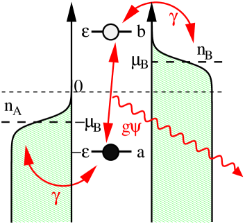
Figure 2: (Color online) Schematic diagram illustrating occupation of A and B baths, and their coupling to the two fermionic levels. In the case shown, the bath chemical potential is below the energy level $\epsilon$, so the pumping cannot lead to inversion. The flow of energy is from the pumping bath, through the fermionic levels of an exciton, to the photons, and energy is then lost into the photon bath.

Before proceeding further, let us examine what the form of the self energy due to the bath tells us about the relation between thermalisation and dephasing. In principle one could consider a non-Markovian environment where for some range of frequencies one has $\gamma(\omega)=0$, $\kappa(\omega)=0$. Then, for that range, there would be no damping, but also $p^{K}(\omega)=0$, $d^{K}(\omega)=0$, so the system distribution in such a range would not be influenced by the bath — i.e. no thermalisation. Thus for a full thermalisation of all relevant modes of the system, one needs a non-zero coupling to the low frequency modes of the environment, which will at the same time introduce dephasing.

III.2 Integration over fermionic fields

After eliminating the bath’s degrees of freedom the full action $S$ becomes

$$S=\int_{-\infty}^{\infty}dtdt^{\prime}\left[\sum_{\alpha,\alpha^{\prime}}\bar{\phi}_{\alpha}(t)G_{\alpha,\alpha^{\prime}}^{-1}(t,t^{\prime})\phi_{\alpha^{\prime}}(t^{\prime})\right.\\ +\left.\sum_{\mathbf{p}}\bar{\psi}_{\mathbf{p}}(t)\left(\begin{array}[]{cc}0&i\partial_{t}-\omega_{\mathbf{p}}-i\kappa\\ i\partial_{t}-\omega_{\mathbf{p}}+i\kappa&2i\kappa F_{\Psi}(t-t^{\prime})\end{array}\right)\psi_{\mathbf{p}}(t^{\prime})\right],$$

where $G$ is the exciton Green’s function. Introducing the abbreviations $\lambda_{cl}=\sum_{{\mathbf{p}}}\frac{g_{{\mathbf{p}},\alpha}}{\sqrt{2}}\psi_{{\mathbf{p}},cl}$ and $\lambda_{q}=\sum_{{\mathbf{p}}}\frac{g_{{\mathbf{p}},\alpha}}{\sqrt{2}}\psi_{{\mathbf{p}},q}$ we may write $G$ as:

$$G_{\alpha,\alpha^{\prime}}^{-1}(t,t^{\prime})=\\ \left(\begin{array}[]{cc}(\lambda_{q}(t)\sigma_{+}+\bar{\lambda}_{q}(t)\sigma_{-})\delta_{\alpha,\alpha^{\prime}}&(\partial_{t}\sigma_{0}-\epsilon_{\alpha}\sigma_{3}-\lambda_{cl}(t)\sigma_{+}-\bar{\lambda}_{cl}(t)\sigma_{-})\delta_{\alpha,\alpha^{\prime}}-i\gamma\sigma_{0}\\ (i\partial_{t}\sigma_{0}-\epsilon_{\alpha}\sigma_{3}-\lambda_{cl}(t)\sigma_{+}-\bar{\lambda}_{cl}(t)\sigma_{-})\delta_{\alpha,\alpha^{\prime}}+i\gamma\sigma_{0}&-(\lambda_{q}(t)\sigma_{+}+\bar{\lambda}_{q}(t)\sigma_{-})\delta_{\alpha,\alpha^{\prime}}+2i\gamma(F_{b}\sigma_{\uparrow}+F_{a}\sigma_{\downarrow})\end{array}\right),$$ (7)

Note that $F_{b}(t-t^{\prime})$, $F_{a}(t-t^{\prime})$ as well as $i\partial_{t}$ are time non-local. It is now explicit how the competition between the two environments works. The photon environment, with the distribution function $F_{\Psi}$ of modes outside of the cavity, affects the free photon evolution. Similarly, the fermionic environment, with the bath distributions $F_{b},F_{a}$, enters the exciton Green’s function, now also modified by the presence of cavity photons. The spectrum of this coupled system will combine both the strong coupling between excitons and photons as well as the dissipation to the environment. The occupation of these modes will be a non-trivial combination of the distributions of the baths as well as the exciton-photon interaction.

The action S is quadratic in fermionic fields and therefore it is possible to integrate over the fermionic degrees of freedom $\phi$ and, in the same spirit as in previous studies of the equilibrium properties of this model Eastham ; Szymanska ; Keeling ; Marchetti , obtain the total effective action for the photon field alone

$$S=-i\sum_{\alpha}{\rm Trln}G_{\alpha,\alpha}^{-1}+\int_{-\infty}^{\infty}dtdt^{\prime}\sum_{{\mathbf{p}}}\\ \bar{\psi}_{\mathbf{p}}(t)\left(\begin{array}[]{cc}0&i\partial_{t}-\omega_{\mathbf{p}}-i\kappa\\ i\partial_{t}-\omega_{\mathbf{p}}+i\kappa&2i\kappa F_{\Psi}(t-t^{\prime})\end{array}\right)\psi_{\mathbf{p}}(t^{\prime})$$ (8)

Other than those approximations explicitly discussed in the text, this expression is exact; i.e. it makes no assumption about what form $\psi_{{\mathbf{p}}}(t)$ takes. Note, however, that due to the non-linear term ${\rm Trln}G_{\alpha,\alpha}^{-1}$ the action is highly complex and contains all powers of $\psi_{cl}$ and $\psi_{q}$. Therefore some expansion scheme needs to be performed.

IV Saddle-Point (Mean-Field) Analysis

In order to determine the state of the pumped, decaying, strongly coupled system, we will follow a standard method for path integrals, and first find the saddle point solution. The saddle-point equations for the action (8) have the following form

$$\frac{\delta S}{\delta\bar{\psi}_{{\mathbf{p}},q}}=\int dt^{\prime}\biggl{\{}\left[(i\partial_{t}-\omega_{\mathbf{p}})\delta(t-t^{\prime})-d^{R}(t-t^{\prime})\right]\psi_{{\mathbf{p}},cl}(t^{\prime})\biggr{.}\\ \biggl{.}-d^{K}(t-t^{\prime})\psi_{{\mathbf{p}},q}(t^{\prime})\biggr{\}}-\sum_{\alpha}\frac{g_{{\mathbf{p}},\alpha}}{\sqrt{2}}(-i){\rm Tr}(G_{\alpha,\alpha}\sigma_{-}\sigma_{0}^{\textsc{k}})=0,$$

$$\frac{\delta S}{\delta\bar{\psi}_{{\mathbf{p}},cl}}=\int dt^{\prime}\left[(i\partial_{t}-\omega_{\mathbf{p}})\delta(t-t^{\prime})-d^{A}(t-t^{\prime})\right]\psi_{{\mathbf{p}},q}(t^{\prime})\\ -\sum_{\alpha}\frac{g_{{\mathbf{p}},\alpha}}{\sqrt{2}}(-i){\rm Tr}(G_{\alpha,\alpha}\sigma_{-}\sigma_{1}^{\textsc{k}})=0.$$

It can be seen that the second equation is satisfied by $\psi_{{\mathbf{p}},q}=0$ (classical saddle-point). Putting $\psi_{{\mathbf{p}},q}=0$ into (7) gives the usual structure for the mean-field exciton Green’s function, which ensures causality Kamenev :

$$G^{-1}=\left(\begin{array}[]{cc}0&[G^{A}]^{-1}\\ \left[G^{R}\right]^{-1}&\left[G^{-1}\right]^{K}\end{array}\right)$$

and so $G=\left(\begin{array}[]{cc}G^{K}&G^{R}\\ G^{A}&0\end{array}\right),$ where $G^{K}=-G^{R}[G^{-1}]^{K}G^{A}$. It is now clear why the Keldysh rotation discussed earlier, i.e. working in terms of $(cl,q)$ components rather than $(f,b)$, is more convenient. By reducing the number of dependent functions, both the Green’s function and inverse Green’s function contain a zero block, and so become easier to invert. With this structure ${\rm Tr}(G\sigma_{-}\sigma_{0}^{\textsc{k}})={\rm Tr}(G^{K}\sigma_{-})$ and ${\rm Tr}(G\sigma_{-}\sigma_{1}^{\textsc{k}})={\rm Tr}((G^{R}+G^{A})\sigma_{-})=0$ since $G^{R}(t,t)+G^{A}(t,t)=0$. Thus we are left with only the first of the saddle point equations, which now becomes:

$$\int dt^{\prime}\left[(i\partial_{t}-\omega_{\mathbf{p}})\delta_{t-t^{\prime}}-d^{R}(t-t^{\prime})\right]\psi_{{\mathbf{p}},cl}(t^{\prime})=\\ \sum_{\alpha}\frac{g_{{\mathbf{p}},\alpha}}{\sqrt{2}}(-i){\rm Tr}(G_{\alpha,\alpha}^{K}\sigma_{-}).$$

Since we consider an infinite homogeneous system (no trap) we expect a uniform saddle point. We therefore consider the solutions to be of the form $\psi_{\mathbf{p}}=\psi\delta(p)$. It is difficult to invert $[G^{-1}]^{R,A}$ matrix for an arbitrary time dependence of the $\psi$ fields. We are, however, interested in the non-equilibrium steady-state so we take the only time dependence of the photon field $\psi$ to be oscillation at a single frequency. Therefore we propose the following ansatz

$$\psi(t)=\psi e^{-i\mu_{S}t}.$$ (9)

Substituting this ansatz in the action of Eq. (8) will lead to explicit time dependence within the exciton inverse Green’s function. This time dependence can be removed straightforwardly by implementing an appropriate gauge transformation, described by the following matrix in particle-hole space:

$$U=\left(\begin{array}[]{cc}e^{i\frac{\mu_{S}}{2}t}&0\\ 0&e^{-i\frac{\mu_{S}}{2}t}\end{array}\right)$$

The trace is invariant under unitary transformations, ${\rm Tr}\ln G^{-1}={\rm Tr}\ln UG^{-1}U^{\dagger}$, so the effects of such time-dependence appear in only two places: Firstly in the time derivative terms, which lead to the energy shifts $\omega_{\mathbf{p}}\to\tilde{\omega}_{\mathbf{p}}=\omega_{\mathbf{p}}-\mu_{s}\ \ {\rm and}\ \ \epsilon_{\alpha}\to\tilde{\epsilon}_{\alpha}=\epsilon_{\alpha}-\mu_{s}/2,$ and secondly in a gauge transformation of the bath functions $d^{R/A/K}(\omega)\to d^{R/A/K}(\omega+\mu_{S}),$ $p_{b}^{R/A/K}(\nu)\to p_{b}^{R/A/K}(\nu+\frac{\mu_{S}}{2})\ \ {\rm and}\ \ p_{a}^{R/A/K}(\nu)\to p_{a}^{R/A/K}(\nu-\frac{\mu_{S}}{2}).$ In practice, the latter substitutions mean replacing $\mu_{B}\to\tilde{\mu}_{B}=\mu_{B}-\mu_{S}/2$ in $F_{a},F_{b}$.

With $\psi_{q}=0$ and the above time-dependence described by the gauge transformation, the matrix $G^{-1}$ can now be easily inverted and the final form for the mean-field exciton Green’s functions are

$$G^{R/A}(\nu)=\frac{(\nu\pm i\gamma)\sigma_{0}+\tilde{\epsilon}_{\alpha}\sigma_{3}+g\psi_{f}\sigma_{+}+g\bar{\psi}_{f}\sigma_{-}}{\nu^{2}-E_{\alpha}^{2}\pm 2i\gamma\nu-\gamma^{2}},$$ (10)

and

$$G^{K}_{bb/aa}(\nu)\!=\!-2i\gamma\frac{F_{b/a}(\nu)[(\nu\!\pm\!\tilde{\epsilon}_{\alpha})^{2}\!+\!\gamma^{2}]+F_{a/b}(\nu)g^{2}|\psi_{f}|^{2}}{[(\nu-E_{\alpha})^{2}+\gamma^{2}][(\nu+E_{\alpha})^{2}+\gamma^{2}]},$$ (11)

$$G^{K}_{ba}(\nu)=-(G^{K}_{ab}(\nu))^{\ast}=-2i\gamma g\psi_{f}\times\\ \frac{(F_{a}(\nu)+F_{b}(\nu))\nu+(F_{b}(\nu)-F_{a}(\nu))(\tilde{\epsilon}_{\alpha}+i\gamma)}{[(\nu-E_{\alpha})^{2}+\gamma^{2}][(\nu+E_{\alpha})^{2}+\gamma^{2}]},$$ (12)

where $a$, $b$ defines the particle-hole space as follows

$$G=\left(\begin{array}[]{cc}G_{bb}&G_{ba}\\ G_{ab}&G_{aa}\end{array}\right),$$

and $E_{\alpha}=\sqrt{\tilde{\epsilon}_{\alpha}^{2}+g^{2}|\psi_{f}|^{2}}$. Note that only the site-index diagonal, i.e. ($\alpha$,$\alpha$), component appears in the gap equation and so we have omitted the site index in G for brevity. Also since at the saddle point $\psi_{q}=0$ then $\psi_{f}=\frac{\psi_{cl}+\psi_{q}}{\sqrt{2}}=\frac{\psi_{cl}}{\sqrt{2}}$. In this work we consider $g_{{\mathbf{p}},\alpha}=g$. The influence of the distribution of the oscillator strength has been addressed in Ref. Marchetti, . The mean-field exciton Green’s functions physically correspond to excitons strongly renormalised by the presence of the mean-field photon field, and damped by the coupling to the environment. The Keldysh Green’s function, which contains the distribution of excitons, depends on the distributions of the pumping bath. In general

$$G^{K}=G^{R}F-FG^{A},$$

where $F$ has a meaning of the quasi-particle distribution function. We can determine the mean-field distribution function for excitons in a self-consistent photon field from Eqs. (10)–(12):

$$F_{bb/aa}(\nu)=\frac{F_{a}(\nu)+F_{b}(\nu)}{2}\pm\frac{(F_{b}(\nu)-F_{a}(\nu))(\tilde{\epsilon}_{\alpha}^{2}+\gamma^{2})}{2(E_{\alpha}^{2}+\gamma^{2})},$$

$$F_{ba}(\nu)=(F_{ab})^{\ast}(\nu)=\frac{g\psi_{f}(F_{b}(\nu)-F_{a}(\nu))(\tilde{\epsilon}_{\alpha}+i\gamma)}{2(E_{\alpha}^{2}+\gamma^{2})},$$

where $F_{a}$ and $F_{b}$ are the bath’s distributions given by Eq. (6), with $\mu_{B}\to\tilde{\mu}_{B}$. Note that, since this is a mean-field approximation, only coherent photons enter in this distribution. Thus, in the uncondensed case where $\psi=0$ the exciton distributions reduce to $F_{bb/aa}=F_{b/a}$ and $F_{ab}=0$: i.e. in the absence of coherent photons, the mean field approximation neglects the effect of photons on the exciton distribution. The distribution of the photonic environment will however enter the distribution of fluctuations about the mean-field, as will be discussed in Sec. V.1.

With the ansatz (9) the saddle-point equation becomes

$$(\omega_{0}-\mu_{S}-i\kappa)\psi_{f}=\sum_{\alpha}\frac{g}{2}(-i){\rm Tr}(G_{ba}^{K}).$$ (13)

As in equilibrium this is a self-consistent equation for the order parameter (condensate). With changing density the type of transition moves from interaction dominated BCS-like mean-field regime to a fluctuation dominated BEC limitKeeling (strictly speaking BKT in 2D) . So the above equation is analogous to the gap equation in the theory of BCS-BEC crossover. Here it relates the coherent photon field with the exciton Green’s function strongly modified by the presence of such a coherent field. Physically it means that the coherent field is generated by a coherent polarisation in the exciton system which in turn is generated by the presence of the coherent field. Thus equation (13) can be viewed as a non-equilibrium generalisation of the gap equation. One difference with respect to equilibrium is that the distribution function contained in $G^{K}$ now may not be thermal. However, the more important difference is that the gap equation (13) is now complex and gives two equations for two unknowns: the order parameter $\psi$ and the frequency $\mu_{S}$.

The common oscillation frequency $\mu_{S}$ would in thermal equilibrium be the system’s chemical potential, considered as a control parameter, adjusted to match the required density, and the (real) gap equation determines only $\psi$. Here, because different baths have different chemical potentials, the system is not in chemical equilibrium with either bath, so both $\mu_{S}$ and $\psi$ must be found from the gap equation. The density, which can be found given $\psi$ and $\mu_{S}$, is set by the relative strength of the pump and decay.

Thus the real part of the gap equation is analogous to the gap equation for closed equilibrium system, where the right hand side describes polarisation due to nonlinear susceptibility. By considering the existence of pumping and decay, one also introduces the imaginary part, which describes how the gain balances the decay (as in lasers) but now in the strongly coupled exciton-photon system. If one were to instead consider the equilibrium theory, and merely add decay rates, one could not a priori guarantee that the fluctuation spectrum would be gapless, as should arise from spontaneous symmetry breaking. By ensuring that gain and decay balance, the fluctuation spectrum above the ground state which satisfies both the real and imaginary parts of the gap equation, will indeed be gapless. By connecting the equilibrium self consistency condition (gap equation, Gross Pitaevskii equation), and the laser rate equation, Eq. (13) puts the condensate and the laserHaken:RMP in the same framework and so allows study of the crossover and the relation between the two.

Using (12) the mean-field equation becomes

$$(\omega_{0}-\mu_{S}-i\kappa)\psi_{f}=\\ \sum_{\alpha}\int\frac{d\nu}{2\pi}\psi_{f}g^{2}\gamma\frac{(F_{a}+F_{b})\nu+(F_{b}-F_{a})(\tilde{\epsilon}_{\alpha}+i\gamma)}{[(\nu-E_{\alpha})^{2}+\gamma^{2}][(\nu+E_{\alpha})^{2}+\gamma^{2}]}.$$ (14)

Note that $\gamma$ appears both in the denominator (as it gives rise to the dephasing) and in the numerator (it gives rise to pumping).

As in thermal equilibrium, the normal state $\psi_{f}=0$ is always a solution of Eq. (14), but for some range of parameters there is also a condensed $\psi_{f}\neq 0$ solution. For $\psi_{f}\neq 0$ the final form of the gap equation is

$$\tilde{\omega}_{0}-i\kappa=\\ g^{2}\gamma\sum_{\alpha}\int\frac{d\nu}{2\pi}\frac{(F_{a}+F_{b})\nu+(F_{b}-F_{a})(\tilde{\epsilon}_{\alpha}+i\gamma)}{[(\nu-E_{\alpha})^{2}+\gamma^{2}][(\nu+E_{\alpha})^{2}+\gamma^{2}]}.$$ (15)

Now for a given set of parameters we can solve the real and imaginary parts of this equation to determine the coherent photon field $\psi_{f}$ and its oscillation frequency $\mu_{S}$.

We can reduce the number of parameters in our theory by measuring energies in units of the exciton-photon coupling $g$ and, noting that our equations have made no assumption about the origin of energies, taking $\epsilon_{0}$ as some reference energy, such as the bottom of the exciton band. The independent parameters in our theory are then the distribution of exciton energies [i.e. $\sum_{\alpha}\to\int d\epsilon\nu_{S}(\epsilon)$], the detuning of the photon from the reference point $\Delta=\omega_{0}-2\epsilon_{0}$, the pumping bath chemical potential $\mu_{B}-\epsilon_{0}$, the pumping (decoherence) strength $\gamma$, and the coupling to the decay bath $\kappa$.

Having found the self consistent oscillation frequency $\mu_{S}$ and coherent field, one can then calculate the excitonic density and polarisation. The polarisation, i.e. $\langle a^{\dagger}b\rangle$ (where $|\langle a^{\dagger}b\rangle|^{2}$ also gives the number of condensed fermion pairs - condensed excitons) follows directly from the gap equation, so the magnitude of polarisation is given by $\sqrt{\tilde{\omega}^{2}+\kappa^{2}}\psi_{f}$. The excitonic density is given by:

$$\sum_{\alpha}\frac{1}{2}\left(b^{\dagger}_{\alpha}b_{\alpha}-a^{\dagger}_{\alpha}a_{\alpha}\right)=\\ \frac{1}{4}i\sum_{\alpha}\int\frac{d\nu}{2\pi}\left(G^{K}_{aa}(\nu)-G^{K}_{bb}(\nu)\right)=\frac{\gamma}{2}\sum_{\alpha}\int\frac{d\nu}{2\pi}\\ \times\frac{(F_{b}-F_{a})\left[g^{2}|\psi|^{2}-\nu^{2}-\tilde{\epsilon}_{\alpha}^{2}-\gamma^{2}\right]-(F_{b}+F_{a})2\nu\tilde{\epsilon}_{\alpha}}{[(\nu-E_{\alpha})^{2}+\gamma^{2}][(\nu+E_{\alpha})^{2}+\gamma^{2}]}.$$ (16)

Since our choice of bath populations in Eq. (6) implies that the empty state corresponds to $\langle b^{\dagger}b\rangle=0$, $\langle a^{\dagger}a\rangle=1$, it will be convenient to shift the exciton density so that the empty state corresponds to zero density, thus:

$$\rho_{\mathrm{exciton}}=\sum_{\alpha}\frac{1}{2}\left(1+b^{\dagger}_{\alpha}b_{\alpha}-a^{\dagger}_{\alpha}a_{\alpha}\right).$$ (17)

In the limit that the temperature of the pumping bath goes to zero, one can perform the various integrals in Eq. (15) and Eq. (16) in terms of elementary functions. These forms are presented in Appendix A.

IV.1 $\gamma=0,\kappa=0$ limit

In order to understand the meaning of the gap equation, and the connection to condensation in a closed equilibrium system, it is instructive to take the limit $\gamma\to 0,\kappa\to 0$ in Eq. (15). This will also provide a consistency check of the non-equilibrium theory as it should recover the equilibrium limit as the coupling to the environment approaches zero. The real part of Eq. (15) can be rewritten as:

$$\omega_{0}-\mu_{S}=\frac{g^{2}}{4E}\int\frac{d\nu}{2\pi}\left[\frac{\gamma}{(\nu-E)^{2}+\gamma^{2}}-\frac{\gamma}{(\nu+E)^{2}+\gamma^{2}}\right]\\ \times\left[(F_{a}(\nu)+F_{b}(\nu))+(F_{b}(\nu)-F_{a}(\nu))\frac{\tilde{\epsilon}_{\alpha}}{\nu}\right].$$

From the definition of the $\delta$ function we have

$$\lim_{\gamma\to 0}\frac{\gamma}{(\nu-E)^{2}+\gamma^{2}}=\pi\delta(\nu-E)$$

and so, using $F_{a}(-\nu)=-F_{b}(\nu)$, the real part of the gap equation reduces to

$$\omega_{0}-\mu_{S}=\frac{g^{2}}{4E}\left[F_{b}(E)+F_{a}(E)\right]\\ +\frac{g^{2}\tilde{\epsilon}}{4E^{2}}\left[F_{b}(E)-F_{a}(E)\right].$$ (18)

Similarly, the imaginary part of the gap equation can be rearranged as:

$$\frac{\kappa}{\gamma}=\frac{g^{2}}{4E^{2}}\left[F_{a}(E)-F_{b}(E)\right].$$ (19)

Let us consider the limit where $\kappa/\gamma\to 0$, i.e. coupling to the photon bath vanishes faster, and so the distribution will be set by the pumping bath. Then the left hand side of Eq. (19) is zero and so one requires $F_{a}(E)=F_{b}(E)$. Using the gauge transformed versions of the thermal distribution functions in Eq. (6), this condition becomes $\tilde{\mu}_{B}=0$, i.e. that $\mu_{S}=2\mu_{B}$. Putting this solution into (18) we recover the equilibrium gap equation at a temperature $T$ set by the pumping bath:

$$\tilde{\omega}_{0}=\frac{g^{2}}{2E}\rm{tanh}\frac{\beta}{2}E.$$

This limit provides a reassuring test of the formalism, and also supports the interpretation that the real part of the gap equation connects the order parameter with non-linear susceptibility, while the imaginary part describes the balance of gain and decay, and so controls $\mu_{S}$ and the particle density in the system.

V Second Order Fluctuations and Stability of Solutions

Having found the self-consistency condition, considering the possibility of uniform condensed solutions, we next consider the stability of such solutions. The consideration of stability is important firstly since, as discussed above, $\psi_{f}=0$ is always a solution of Eq. (13), so one must determine which of the normal and condensed solutions is stable, and secondly because we considered only spatially homogeneous fields, with a single oscillation frequency, so one may find that neither $\psi_{f}=0$ nor our ansatz of Eq. (9) is stable, suggesting more interesting behaviour. There is an important difference in interpretation of the saddle point equation between the closed-time-path path-integral formalism used here, and the imaginary-time path-integral in thermal equilibrium. In the imaginary time formalism, extremising the action corresponds to finding configurations which extremise the free energy; thus, stable solutions correspond to a minimum of free energy, and unstable to local maxima. Here in contrast, for a classical saddle point (i.e. $\psi_{q}=0$), the action is always $S=0$, and the saddle point condition corresponds to configurations for which nearby paths add in phase. Thus, in order to study stability one must directly investigate fluctuations about our ansatz, and determine whether such fluctuations grow or decay.

In considering the question of stability, we will first discuss stability of the normal state, which is instructive as it shows how the question of whether fluctuations about the non-equilibrium steady-state grow or decay is directly related to the instability expected in thermal equilibrium systems when the chemical potential goes above a bosonic mode. We will then turn to the spectrum of fluctuations about our condensed ansatz. While we will discuss here whether such fluctuations are stable or unstable, we will defer until Sec. VII the evaluation of correlation functions associated with these fluctuations. This is because, as discussed there, these fluctuations include phase modes, and phase fluctuations may become large. It is therefore insufficient to only expand to second order in fluctuation fields, but one must instead reparameterise $\psi=\sqrt{\rho_{0}+\pi}e^{i\phi}$, and then describe the correlation functions of $\psi$ in terms of those of phase $\phi$ and amplitude $\pi$, including the effects of $\phi$ to all orders. Such a complication is however not needed in order to study whether fluctuations are stable or not, and so it is reasonable to postpone such a treatment, and consider an expansion in terms of $\psi=\psi_{0}+\delta\psi$ to second order in $\delta\psi$ instead.

Thus, to find the spectrum of fluctuations, we consider the effective action governing fluctuations about either $\psi=\psi_{0}$ or about $\psi=0$. Considering the effective action in Eq. (8), and expanding to second order in $\delta\psi$, one finds a contribution from the effective photon action, and a contribution from expanding the trace over excitons. This latter contribution can be found by writing $G_{\alpha,\alpha}^{-1}=(G^{\mathrm{sp}}_{\alpha,\alpha})^{-1}+\delta G_{\alpha}^{-1},$ where $G^{\mathrm{sp}}$ is the saddle point fermionic Green’s function, which depends on the value of the saddle point field $\psi_{f}$, as given in Eq. (10), (11) and (12), and the contribution of fluctuations $\delta{G}_{\alpha}^{-1}$ is given by:

$$\delta G^{-1}=\frac{-1}{\sqrt{2}}(g\delta\bar{\psi_{q}}\sigma_{-}+g\delta\psi_{q}\sigma_{+})\sigma_{0}^{\textsc{k}}+\\ \frac{-1}{\sqrt{2}}(g\delta\bar{\psi}_{cl}\sigma_{-}+g\delta\psi_{cl}\sigma_{+})\sigma_{1}^{\textsc{k}}.$$

Thus, one can expand the action as:

$$-i\sum_{\alpha}{\rm Trln}\left[G_{\alpha,\alpha}^{-1}\right]=(-i)\sum_{\alpha}{\rm Trln}\left[(G^{\mathrm{sp}}_{\alpha,\alpha})^{-1}\right]\\ +(-i)\sum_{\alpha}{\rm Tr}\left[G^{\mathrm{sp}}_{\alpha,\alpha}\delta G_{\alpha}^{-1}\right]\\ +(-i)(-\frac{1}{2})\sum_{\alpha}{\rm Tr}\left[G^{\mathrm{sp}}_{\alpha,\alpha}\delta G_{\alpha}^{-1}G^{\mathrm{sp}}_{\alpha,\alpha}\delta G_{\alpha}^{-1}\right].$$

In this expansion, we have retained only the terms diagonal in site index; i.e. neglected any bath induced interaction between different exciton sites. Such bath induced interactions should be small for small $\gamma$, and their inclusion would considerably complicate the formalism. Such an approach is also equivalent to considering a separate set of baths for each disorder localised state $\alpha$.

Because, in the presence of a coherent field, the effective action can contain terms like $\delta\psi\delta\psi$ and $\delta\bar{\psi}\delta\bar{\psi}$, it is convenient to introduce a Nambu structure of photon fields. Thus, the photon fluctuations are described by a $2\times 2=4$ component vector, with one factor of $2$ from the Keldysh structure, and one from the Nambu structure, hence:

$$\delta\Lambda=\left(\begin{array}[]{c}\delta\psi_{cl}(\omega)\\ \delta\bar{\psi}_{cl}(-\omega)\\ \delta\psi_{q}(\omega)\\ \delta\bar{\psi}_{q}(-\omega)\end{array}\right),$$ (20)

in terms of which the action for fluctuations $\delta S_{f}$ is:

$$\delta S_{f}=\int\frac{d\omega}{2\pi}\delta\bar{\Lambda}(\omega)\left(\begin{array}[]{cc}0&\left[{\cal D}^{-1}\right]^{A}\\ \left[{\cal D}^{-1}\right]^{R}&\left[{\cal D}^{-1}\right]^{K}\end{array}\right)\delta\Lambda(\omega).$$

For convenience later, we shall introduce the notation:

$$\left[{\cal D}^{-1}\right]^{R/A/K}=\left(\begin{array}[]{cc}K^{R/A/K}_{1}&K^{R/A/K}_{2}\\ \\ K^{R/A/K}_{3}&K^{R/A/K}_{4}\end{array}\right).$$ (21)

By definition we have that: $\left[{\cal D}^{-1}\right]^{A}=\left(\left[{\cal D}^{-1}\right]^{R}\right)^{\dagger}$, and in addition the Nambu structure implies certain symmetries between the elements of $[{\cal D}^{-1}]^{R/A/K}$, which together can be written as:

$$\begin{array}[]{l@{\mbox{}=\mbox{}}l@{\mbox{}=\mbox{}}l@{\mbox{}=\mbox{}}l}K^{R}_{1}(\omega)&K^{A}_{1}(\omega)^{\ast}&K^{R}_{4}(-\omega)^{\ast}&K^{A}_{4}(-\omega)\\[5.16663pt] K^{R}_{2}(\omega)&K^{A}_{2}(-\omega)&K^{R}_{3}(-\omega)^{\ast}&K^{A}_{3}(\omega)^{\ast}\end{array}$$ (22)

$$\begin{split}K^{K}_{2}(\omega)&=-K^{K}_{3}(\omega)^{\ast}=K^{K}_{2}(-\omega)\\ K^{K}_{1}(\omega)&=K^{K}_{4}(-\omega)\end{split}$$ (23)

Introducing the compact notation:

$$[f\ast g]_{\omega}=\int\frac{d\nu}{2\pi}f(\nu)g(\nu-\omega)$$

we may thus write:

$$\left[{\cal D}^{-1}\right]^{R}(\omega,{\mathbf{p}})=\frac{1}{2}\left(\begin{array}[]{cc}\omega-\tilde{\omega}_{{\mathbf{p}}}+i\kappa&0\\ \\ 0&-\omega-\tilde{\omega}_{{\mathbf{p}}}-i\kappa\end{array}\right)+i\frac{g^{2}}{4}\left(\begin{array}[]{ccc}G^{R}_{bb}\ast G^{K}_{aa}+G^{K}_{bb}\ast G^{A}_{aa}&\ \ G^{R}_{ba}\ast G^{K}_{ba}+G^{K}_{ba}\ast G^{A}_{ba}\\ \\ G^{R}_{ab}\ast G^{K}_{ab}+G^{K}_{ab}\ast G^{A}_{ab}&\ \ G^{R}_{aa}\ast G^{K}_{bb}+G^{K}_{aa}\ast G^{A}_{bb}\end{array}\right)_{\omega},$$ (24)

and

$$\left[{\cal D}^{-1}\right]^{K}(\omega,{\mathbf{p}})=\frac{1}{2}\left(\begin{array}[]{cc}2i\kappa F_{\psi}(\omega+\mu_{S})&0\\ \\ 0&2i\kappa F_{\psi}(-\omega+\mu_{S})\end{array}\right)+\\ i\frac{g^{2}}{4}\left(\begin{array}[]{ccc}G^{K}_{bb}\ast G^{K}_{aa}+G^{R}_{bb}\ast G^{A}_{aa}+G^{A}_{bb}\ast G^{R}_{aa}&\ \ G^{K}_{ba}\ast G^{K}_{ba}+G^{R}_{ba}\ast G^{A}_{ba}+G^{A}_{ba}\ast G^{R}_{ba}\\ \\ G^{K}_{ab}\ast G^{K}_{ab}+G^{R}_{ab}\ast G^{A}_{ab}+G^{A}_{ab}\ast G^{R}_{ab}&\ \ G^{K}_{aa}\ast G^{K}_{bb}+G^{R}_{aa}\ast G^{A}_{bb}+G^{A}_{aa}\ast G^{R}_{bb}\end{array}\right)_{\omega}$$ (25)

V.1 Normal state excitation spectra and distributions

The excitation spectrum can be found from the poles of the fluctuation Green’s function, i.e. from the zeros of $\det\left[{\cal D}^{-1}\right]^{R}$. To extract the occupation of the spectrum, one can extract the boson distribution function via

$${\cal D}^{K}=-{\cal D}^{R}\left[{\cal D}^{-1}\right]^{K}{\cal D}^{A}={\cal D}^{R}F_{S}-F_{S}{\cal D}^{A},$$

where simply ${\cal D}^{R/A}=\left[\left[{\cal D}^{-1}\right]^{R/A}\right]^{-1}$. Whilst in general these are $2\times 2$ matrices in Nambu space, in the normal state this structure is redundant, and so the distribution function is the diagonal constant matrix $F_{S}=2n_{S}+1$, where $n_{S}$ describes the occupation of the modes. Alternatively, one can invert the Keldysh rotation in order to find the physical Green’s functions,

$${\cal D}^{<,>}=\frac{1}{2}\left({\cal D}^{K}\mp\left[{\cal D}^{R}-{\cal D}^{A}\right]\right),$$ (26)

which as discussed in Sec. III relate directly to the luminescence, ${\cal L}(\omega,{\mathbf{p}})=i{\cal D}^{<}(\omega,{\mathbf{p}})/2\pi$, and absorption ${\cal A}(\omega,{\mathbf{p}})=i{\cal D}^{>}(\omega,{\mathbf{p}})/2\pi$. Still, assuming the normal state, so that the Nambu structure is redundant, these become:

$${\cal L}(\omega,{\mathbf{p}}) =n_{S}(\omega)\mathrm{Im}\left(-\frac{{\cal D}^{R}(\omega,{\mathbf{p}})}{\pi}\right),$$

$${\cal A}(\omega,{\mathbf{p}}) =\left(n_{S}(\omega)+1\right)\mathrm{Im}\left(-\frac{{\cal D}^{R}(\omega,{\mathbf{p}})}{\pi}\right).$$

While this form illustrates how the spectral weight and occupation can be separately extracted from the luminescence and absorption, in order to study these quantities it is more helpful to write them in terms of the components, $K_{1}^{R,K}$ of the inverse Green’s function. In the normal state, there are no anomalous (off diagonal in Nambu space) contributions, and so $K_{2}^{R/A/K}=K_{3}^{R/A/K}=0$. Thus, the normal state luminescence, absorption, and distribution functions are given by:

$$\left({\cal L},{\cal A}\right)(\omega,{\mathbf{p}}) =\frac{-iK_{1}^{K}(\omega)\mp 2\mathrm{Im}\left[K_{1}^{R}(\omega)\right]}{4\pi|K_{1}^{R}(\omega,{\mathbf{p}})|^{2}},$$ (27)

$$F_{S}(\omega) =\frac{-iK_{1}^{K}(\omega)}{2\mathrm{Im}\left[K_{1}^{R}(\omega)\right]}.$$ (28)

Let us now discuss what can be understood in general from the form of these equations, and then illustrate this discussion with the simple case $\gamma\ll T$. From the difference of luminescence and absorption in Eq. (27), one can identify a spectral weight:

$$2\pi S(\omega,{\mathbf{p}})=\frac{\mathrm{Im}\left[K_{1}^{R}(\omega)\right]}{\mathrm{Re}\left[K_{1}^{R}(\omega,{\mathbf{p}})\right]^{2}+\mathrm{Im}\left[K_{1}^{R}(\omega)\right]^{2}}$$ (29)

thus, if the imaginary part of $K_{1}^{R}(\omega)$ is a smooth function of omega, then one will have almost Lorentzian peaks of the spectral weight at values $\omega^{\ast}$ where $\mathrm{Re}\left[K_{1}^{R}(\omega^{\ast})\right]=0$. The width of these peaks, i.e. the linewidth, is then given by $\mathrm{Im}\left[K_{1}^{R}(\omega^{\ast})\right]$. Thus, the imaginary part plays one role as determining the linewidth. It also plays a second role, since from Eq. (28), a zero of the imaginary part causes the distribution to diverge; however, at these same points Eq. (29) implies the spectral weight vanishes, so the number of photons does not diverge. Since a Bose distribution would diverge at the chemical potential, we can use this as a definition of an effective boson chemical potential, so $\mathrm{Im}\left[K_{1}^{R}(\mu^{\mathrm{eff}})\right]=0$. These results are illustrated in Fig. 3, which show the luminescence, absorption, spectral weight, and distribution function against the real and imaginary parts of $K_{1}^{R}$ and $K_{1}^{K}$.

From the above, it is clear that the form of $\mathrm{Im}\left[K_{1}^{R}(\omega)\right]$ as well as $K_{1}^{K}(\omega)$ conspire to set the effective photon distribution. Using the expressions in Eq. (10), (11), and (12), and for the moment restricting to the case $\epsilon_{\alpha}=\epsilon$ we may write:

$$-iK_{1}^{K}(\omega) =\kappa F_{\Psi}(\omega)+\frac{g^{2}}{4}\left[2\mathrm{Re}\int\frac{d\nu}{2\pi}\frac{1}{(\nu-\tilde{\epsilon}+i\gamma)(\nu-\omega+\tilde{\epsilon}-i\gamma)}-4\gamma^{2}\int\frac{d\nu}{2\pi}\frac{F_{b}(\nu)F_{a}(\nu-\omega)}{\left[(\nu-\tilde{\epsilon})^{2}+\gamma^{2}\right]\left[(\nu-\omega+\tilde{\epsilon})^{2}+\gamma^{2}\right]}\right]$$ (30)

$$2\mathrm{Im}\left[K_{1}^{R}(\omega)\right] =\kappa+g^{2}\gamma^{2}\int\frac{d\nu}{2\pi}\frac{F_{b}(\nu)-F_{a}(\nu-\omega)}{\left[(\nu-\tilde{\epsilon})^{2}+\gamma^{2}\right]\left[(\nu-\omega+\tilde{\epsilon})^{2}+\gamma^{2}\right]}.$$ (31)

For the case of pumping baths being individually in thermal equilibrium, one may get some insight into how the pump and decay baths compete to set the systems distribution.

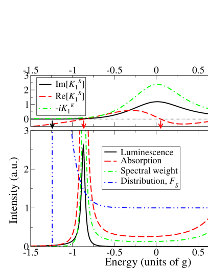
Figure 3: (Color online) Relation between real and imaginary parts of $K_{1}^{R}$ and $K_{1}^{K}$ and the luminescence, absorption, spectral weight and distribution function. Plotted for $\gamma=0.2g,\kappa=0.02g,T=0.1g,\mu_{B}=-0.5g$. (cf Fig. 4) The upper panel shows the real and imaginary parts of $K_{1}^{R}$, and their zeros marked by arrows. The lower panel shows how these lead to peaks in the luminescence spectrum, and how the zero of $\mathrm{Im}[K^{1}_{R}]$ defines divergence of the distribution function.

In the limit $\gamma\ll T$, where $T$ is the temperature of the pumping bath, the distribution functions $F_{b/a}(\nu)$ are smooth, while the denominators lead to sharp peaks, of width $\gamma$. One can then approximate the integrals by assuming that over each Lorentzian peak, the distribution function takes its value at the maximum of that peak, and so:

$$F_{S}(\omega)=\frac{\displaystyle\kappa F_{\Psi}(\omega)+\frac{g^{2}\gamma\left(1-F_{b}(\tilde{\epsilon})F_{a}(\tilde{\epsilon}-\omega)\right)}{(\omega-2\tilde{\epsilon})^{2}+4\gamma^{2}}}{\displaystyle\kappa+\frac{g^{2}\gamma\left(F_{b}(\tilde{\epsilon})-F_{a}(\tilde{\epsilon}-\omega)\right)}{(\omega-2\tilde{\epsilon})^{2}+4\gamma^{2}}}$$ (32)

From this one can see immediately two trivial limits. If $\gamma=0$ or if $g=0$, then there is no influence of the pumping bath and so $F_{S}(\omega)=F_{\Psi}(\omega)$, i.e the photon distribution in the system is the same as the distribution of bulk modes outside the cavity. Similarly, if $\kappa=0$, the photon bath has no effect, and

$$F_{S}(\omega)=\frac{1-F_{b}(\tilde{\epsilon})F_{a}(\tilde{\epsilon}-\omega)}{F_{b}(\tilde{\epsilon})-F_{a}(\tilde{\epsilon}-\omega)}.$$

Thus, as one might expect, if the fermions are in thermal equilibrium with $F_{b,a}(\nu)=F(\nu\mp\tilde{\mu}_{B})$ where $F(\nu)=\tanh(\beta\nu/2)$, then by using a standard hyperbolic trigonometric identity, this gives a thermal Bose distribution for the photons, with the same temperature, but twice the chemical potential, as expected since one boson corresponds to two fermions:

$$F_{S}(\omega) =\coth\left[\frac{\beta}{2}\left(\tilde{\epsilon}-\tilde{\mu}_{B}\right)-\frac{\beta}{2}\left(\tilde{\epsilon}-\omega+\tilde{\mu}_{B}\right)\right]$$

$$=\coth\left[\frac{\beta}{2}\left(\omega-2\tilde{\mu}_{B}\right)\right].$$

The above expressions have been written after the gauge transformation described following Eq. (9). Of course, in the normal state, such a gauge transform has no effect, since it just corresponds to an arbitrary shift of the origin for measuring energies, but we use the transformed notation for consistency with the condensed case.

More generally, the two distributions compete to control the photon distribution, which in general will not be thermal even if the baths are individually thermal, because they have different chemical potentials and temperatures. It is clear from Eq. (32) that the effect of the pumping bath is largest near $\omega=2\tilde{\epsilon}$, and far from this value, both numerator and denominator are instead dominated by the photon bath. Physically, this means that the effect of the pumping bath is only important at energies where the photons are nearly resonant with, and so couple strongly to, the excitons.

V.2 Instability of the normal state above the transition

The discussion in the previous section, which defined $\mu^{\mathrm{eff}}$ by zeros of the imaginary part of $K_{1}^{R}$, and $\omega^{\ast}$ by zeros of the real part allows one to understand the instability of the normal state. It can be seen that the gap equation, (15), if evaluated at $\psi_{f}=0$, is equivalent to the condition $K_{1}^{R}(\omega=0,{\mathbf{p}}=0)=0$, (measuring $\omega$ relative to $\mu_{S}$). This can be understood physically by seeing that the vanishing of $K_{1}^{R}(\omega=0,{\mathbf{p}}=0)$ implies there is a zero mode, corresponding to global phase rotations, as one expects in a broken symmetry system. Thus, this condition implies that there is a frequency at which both real and imaginary parts simultaneously vanish; i.e. the gap equation is the condition that $\mu^{\mathrm{eff}}=\omega^{\ast}$, the effective chemical potential reaches the bottom of the normal mode spectrum. One can say “bottom of the spectrum” since the ${{\mathbf{p}}}$ dependence only enters the real part of $K_{1}^{R}$, and $\omega^{\ast}$ will increase as ${{\mathbf{p}}}$ increases, thus if $\omega^{\ast}_{{\mathbf{p}}=0}<\mu^{\mathrm{eff}}$, then there will be a non-zero ${{\mathbf{p}}}$ for which $\omega^{\ast}_{{\mathbf{p}}}=\mu^{\mathrm{eff}}$. Thus, the existence of a non-trivial solution to the gap equation can still be understood as a “chemical potential” reaching the bottom of the bandZimmermann06 , even in this non-equilibrium context, as is illustrated in Fig. 4.

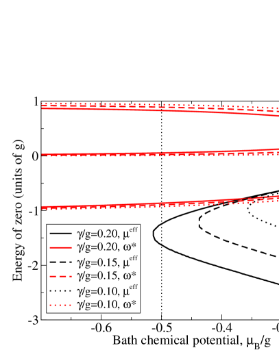
Figure 4: (Color online) Energy of zeros of the real and imaginary part of $K_{1}^{R}$ as a function of $\mu_{B}$, demonstrating how $\mu^{\mathrm{eff}}$, the zero of $\mathrm{Im}(K_{1}^{R})$ approaches $\omega^{\ast}$, a zero of $\mathrm{Re}[K_{1}^{R}]$ at the transition. Results are plotted for $\kappa=0.02g,T_{B}=0.1g$, and three values of $\gamma$ as indicated. The dotted vertical line marks the locations of the trace plotted in Fig. 3

It is also possible to connect the effective chemical potential reaching the bottom of the band to instability of the normal state, i.e. fluctuations growing in time. Let us consider poles, $\xi_{{\mathbf{p}}}$ of the retarded Green’s function, i.e. zeros of $K_{1}^{R}(\xi_{{\mathbf{p}}},{\mathbf{p}})$. If these poles have negative imaginary parts they correspond to fluctuations that decay in time, and if positive, to growing fluctuations; thus stability requires the imaginary part to be always negative. It is clear that at large enough momenta, the Green’s function is that of bare photons, and is stable. Thus, if there are to be unstable modes, then there must be some ${{\mathbf{p}}}$ value at which the imaginary part of the poles goes from negative to positive. For reasonable systems, where the linewidth is a smooth function of momentum, this means the imaginary part must go through zero. A zero of $\mathrm{Im}[\xi_{{\mathbf{p}}}]$ means there is a real frequency which satisfies $K_{1}^{R}(\xi_{{\mathbf{p}}},{\mathbf{p}})=0$. However, the existence of a real frequency satisfying this condition was, as discussed previously, exactly the gap equation at $\psi=0$. Thus, if $\xi_{{\mathbf{p}}}=\omega^{\ast}_{{\mathbf{p}}}=\mu^{\mathrm{eff}}$ for some $|{\mathbf{p}}|=p_{c}$, then for $|{\mathbf{p}}|<p_{c}$ one will find positive imaginary parts. To illustrate this, consider a linear expansion in $\omega$, so that:

$$K_{1}^{R}(\omega,{\mathbf{p}})\simeq(\omega-\omega^{\ast}_{{\mathbf{p}}})+i\alpha(\omega-\mu^{\mathrm{eff}})\simeq C(\omega-\xi_{{\mathbf{p}}}),$$

then one finds, $\mathrm{Im}\xi_{{\mathbf{p}}}\propto(\mu^{\mathrm{eff}}-\omega^{\ast}_{{\mathbf{p}}})$.

Two more important connections can be drawn from the relation between poles of the retarded Green’s function, the distribution, and the gap equation. The first is that, as for any second-order phase transition, approaching the phase transition from the normal side, the fluctuation Green’s function describes a susceptibility which diverges at the transition. The second relates to the dual role that $\mathrm{Im}\left[K_{1}^{R}(\omega^{\ast}_{{\mathbf{p}}})\right]$ played as the linewidth. As one approaches the phase boundary, at which real and imaginary parts both have zeros, one must have that the effective linewidth vanishes. These points are illustrated in Fig. 5. Note however that $\mathrm{Im}\left[K_{1}^{R}(\omega)\right]$ is of course not a constant, and so there will be some non-trivial lineshape, but a linewidth defined by full width half maximum will vanish on approaching the condensed state, as a peak develops at $\omega=0$. The vanishing of homogeneous linewidth at the transition is a manifestation of diverging susceptibility in an infinite system. Finite system size is expected to smear out this divergence and result in the homogeneous linewidth remaining non-zero, but still having a minimum near the transition. Additionally inhomogeneous broadening of exciton energies will add to the linewidth measured in experiments.

Figure 5: (Color online) Linewidth of the lower mode (solid, left axis), and energy integrated luminescence ${\mathbf{p}}_{\parallel}=0$ (dashed, right axis) in the normal state as a function of pumping bath chemical potential, as the phase boundary is approached. Results are shown for two different dephasing parameters $\gamma$ with $\kappa=0.02g$ for all three.

V.3 Fluctuations in condensed state - stability and collective modes

From the previous section we conclude that when there is a non-trivial solution to the gap equation, the normal state is unstable. We wish now to determine whether our ansatz of Eq. (9) is stable. As discussed above, if there were a region with unstable modes (i.e. positive imaginary parts of poles), then this would lead to the existence of a true pole at real omega, at the boundary of the unstable region. Making use of the symmetries in Eq. (22), for the condensed case, poles of the retarded Green’s function correspond to solutions of

$$K_{1}^{R}(\omega,{\mathbf{p}})K_{1}^{R}(-\omega,{\mathbf{p}})^{\ast}-K_{2}^{R}(\omega)K_{2}^{R}(-\omega)^{\ast}=0.$$ (33)

Unfortunately this expression is not simple, and numerical evaluation would be necessary to trace the behaviour of all zeros as a function of momentum. However, in order to understand the stability, we can instead consider separately zeros of the real and imaginary parts of Eq. (33). If zeros of these two parts coincide for some $p_{c}$ , there is a real pole, and thus instability for $|{\mathbf{p}}|<p_{c}$. It is clear the imaginary part should have a zero at $\omega=0$ (measuring frequency from the common oscillation frequency $\mu_{S}$), as the imaginary part of Eq. (33) is an odd function of $\omega$. This zero physically corresponds to the divergence of the distribution function at $\omega=0$. Numerical investigation suggests that this is the only zero of the imaginary part. Thus, we are interested in zeros of the real part, evaluated at $\omega=0$, but arbitrary ${{\mathbf{p}}}$.

It is clear there is a zero at $\omega=0,{\mathbf{p}}=0$, corresponding to the symmetry under global phase rotations, but being at ${\mathbf{p}}=0$ this does not lead to instability. From this pole, or alternatively working directly from the definitions of $K^{R}$ in Eq. (24), and the gap equation (15), one can show that $K_{1}^{R}(\omega=0,{\mathbf{p}}=0)=K_{2}^{R}(\omega=0)$. Thus, writing $A=\mathrm{Re}\left[K_{1}^{R}(\omega=0,{\mathbf{p}}=0)\right]$, instability occurs if there is a non-zero ${{\mathbf{p}}}$ solution of:

$$\left(A-\frac{1}{2}\frac{{\mathbf{p}}^{2}}{2m_{\mathrm{ph}}}\right)^{2}-A^{2}=\frac{1}{4}\frac{{\mathbf{p}}^{2}}{2m_{\mathrm{ph}}}\left(\frac{{\mathbf{p}}^{2}}{2m_{\mathrm{ph}}}-4A\right)=0,$$

which will exist if and only if $A>0$.

Physically, this says that the Goldstone mode will be unstable for $0<|{\mathbf{p}}|<p_{c}$ if the “static compressibility”, $\mathrm{Re}\left[K_{1}^{R}(0,0)\right]>0$. In equilibrium, the expression for the component $K_{1}^{R}(0,0)$ is real and negative, but including pumping and decay, there are regions where solutions of the gap equation, Eq. (15) exist but which are unstable. Since $\mathrm{Re}\left[K_{1}^{R}(0,0)\right]$ is the real part of the second derivative of the action w.r.t $\psi(\omega=0,k=0)$, it can also be seen as a derivative of the gap equation, thus unstable solutions are characterised by a non-linear susceptibility that increases as coherent field increases.

As a result, there are ranges of the parameters $\kappa,\gamma,\mu_{B}$ for which neither the normal state, nor the ansatz of Eq. (9) are stable. We have not investigated what alternate stable solutions might exist under these conditions, however the existence of a real pole in the response at a non-zero momentum might suggest one should investigate the possibility of a coherent field at non-zero ${\mathbf{p}}$. Such a possibility would not be too surprising, as spontaneous pattern formation is seen in laser systems with a continuum of modesDenz03 .

VI Numerical analysis of the mean-field

VI.1 Phase diagram

Having discussed the conditions under which the uniform, single-frequency condensed solution is stable, we may now consider an effective phase boundary — i.e. find the ranges of parameters for which there is a stable condensed solution. For numerical analysis we choose all baths to be individually in thermal equilibrium. However, as the baths need not be in equilibrium with each other, the system can still be far from thermal equilibrium. Since the cavity photon modes start at energies much above the zero for bulk photon modes, we take the chemical potential of the decay bath to be large and negative. In addition, since at room temperature the population of the bulk photon modes at the energy of cavity modes is negligible, we consider the decay bath to be always at zero temperature. In the following we will first present calculations at zero pumping bath temperature, with a delta function density of states i.e. $\epsilon_{\alpha}=\epsilon$, and at zero detuning. Following that we will then analyse the influence of finite temperature of the pumping baths, and of inhomogeneous broadening of excitons. At zero bath temperature, the bath distributions are entirely defined by their chemical potentials, and so there remain three control parameters, $\mu_{B},\gamma,\kappa$. Note that in this case the pump and decay baths are at the same temperature, but have very different chemical potentials, thus leading to a particle flux through the system, driving it out of equilibrium. In Fig. 6, we illustrate the boundary as a function of $\mu_{B},\gamma,\kappa$ by plotting its section in two planes; the plane of fixed $\kappa$ [Fig. 6(a)], and the plane of fixed $\mu_{B}$ [Fig. 6(b)].

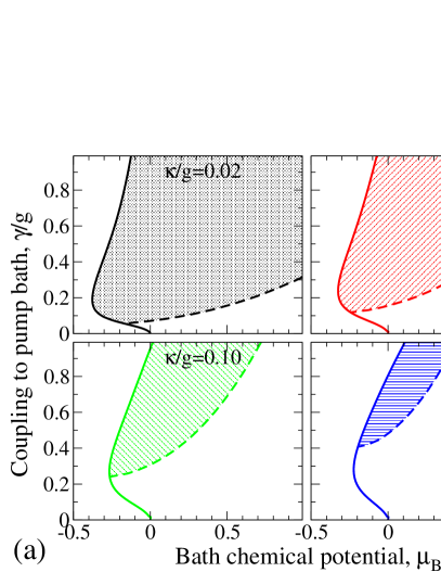
Figure 6: (Color online) Phase boundaries at zero temperature, no inhomogeneous broadening. Panel (a): Fixed decay rate, $\kappa$. Panel (b): Fixed chemical potential, $\mu_{B}$ (Note that $\mu_{B}>0$ implies inversion in the pumping bath but not necessarily in the system). The insets show in detail the region of small $\kappa$ and $\gamma$. Solid lines mark the limit of stability of the normal state. Dashed lines mark the limit of stability between the uniform condensed state, and some other unknown state. The uniform condensed state is stable in the shaded regions. The asterisk in panel (b) marks a point of fixed $\kappa,\gamma$ for comparision between the plots.

It is worth noting that, for $\mu_{B}\leq 0$, and fixed $\kappa,\mu_{B}$ there is both an upper and lower critical $\gamma$. The maximum $\gamma$ is always present (i.e. even if $\mu_{B}>0$), and results because increased coupling to the bath causes dephasing. Let us discuss the origin of the minimum critical $\gamma$. If the bath is at zero temperature, it pumps only that part of the effective excitonic density of states with energy less than the bath chemical potential $\mu_{B}$. If there is no inhomogeneous broadening (i.e. $\epsilon_{\alpha}=\epsilon$) then the effective exciton density of states is set entirely by its coupling to the baths; i.e. it is Lorentzian with width $\gamma$. Thus, the efficiency of pumping depends on how, by broadening the excitonic energy, the pump leads to a non-zero density of states below the chemical potential $\mu_{B}$. As a result, at $\gamma=0$ there is no pumping, and so no condensation, and a minimum $\gamma$ is required before there is sufficient gain to overcome the decay. If there is inhomogeneous broadening of exciton energies, or the pumping baths are at finite temperature, this effect is less significant, as is seen in Fig. 8.

From the boundaries of the stable region, it appears that a uniform condensed stable solution is only possible if $\kappa\leq\kappa_{0}$, with $\kappa_{0}\simeq 0.2g$. The origin of this upper critical $\kappa$ requires further investigation.

VI.2 Coherent fields and densities

As well as the phase boundary, one may study the evolution of a number of properties of the condensate — e.g. mean-field density of condensed photons, $|\psi_{f}|^{2}$, excitonic density [from Eq. (16)], and thus the total mean-field density, being the sum of condensed photon and exciton densities, polarisation $\left<a^{\dagger}b\right>$ (where $|\left<a^{\dagger}b\right>|^{2}$ gives the number of condensed fermion pairs - excitons), and common oscillation frequency $\mu_{S}$. These are shown in Fig. 7, for two values of $\kappa$ and a range of different $\gamma$, chosen to illustrate both the regime of weak coupling to baths, where the results are similar to those in thermal equilibrium, and also strong decay and pumping, for which the results are instead comparable to the laser. For comparison, the value of $\mu^{\mathrm{eff}}$, and the fermion-pair (excitonic) density in the normal state are shown, which connect smoothly to the condensed quantities, as expected for a second order phase transition. Note that for $\kappa=0.15,\gamma=0.9,1.0$ the excitonic density $\rho_{\mathrm{exciton}}>0.5$ indicating inversion as is expected in the lasing case.

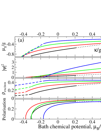
Figure 7: (Color online) Properties of the system as a function of bath chemical potential. Plotted for $T=0$, and $\epsilon_{\alpha}=\epsilon$. Panel (a): $\kappa=0.02g$, panel (b) $\kappa=0.15g$, values of $\gamma$ as indicated. Within each panel, four graphs are shown. Top: The common oscillation frequency in the ansatz of Eq. (9), measured from $\omega_{{\mathbf{p}}=0}=0$; Second: Density of condensed photons; Third: exciton density from Eq. (17); Bottom: Polarisation, given by $\sqrt{\tilde{\omega}^{2}+\kappa^{2}}\psi_{f}$. Solid lines indicate where a stable condensed solution exists; dotted lines are the (unphysical) result of the uniform condensed solution when it is unstable. Dashed lines for $\mu_{S}$ and $\rho_{\mathrm{exciton}}$ show the comparable quantities in the normal state.

VI.3 Influence of bath’s temperatures and excitonic density of states

We now consider the effects of finite bath temperature, and of the inhomogeneous broadening of the exciton energies. As such calculations are numerically intensive, we present a limited, but illustrative set of results. In Fig. 8, the equivalent of Fig. 6(b) is shown, but with a Gaussian density of states, and at small but non-zero temperature of the pumping bath (the decay bath, of bulk photon modes, is still at T=0). One can clearly see that by adding inhomogeneous broadening, $\sigma_{\epsilon}=0.15g$, the lower critical $\gamma$ has been modified, and for large $\mu_{B}$ entirely eliminated. The inset of Fig. 8 shows a higher temperature, for which none of the curves show any lower critical $\gamma$.

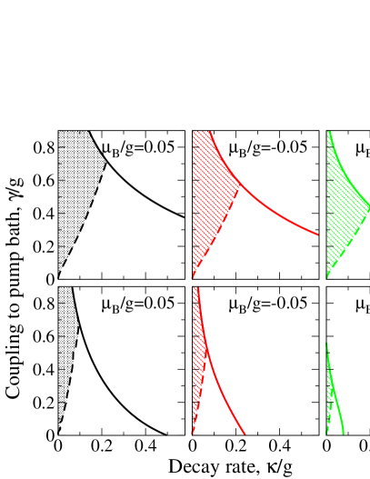
Figure 8: (Color online) Phase boundary for constant chemical potential, $\mu_{B}$, as in Fig. 6(b), but with a Gaussian distribution of excitonic energies, $\sigma_{\epsilon}=0.15g$, and non-zero temperature (top row $T=0.01g$, bottom row $T=0.5g$)

. As a result, the requirement for a minimum coupling strength, $\gamma$, before a transition occurs is removed for some phase boundaries. Solid lines, dashed lines, and shaded region mark instability of normal state, instability of uniform condensed state, and stable condensed region as in Fig. 6.

One can also plot a phase boundary at fixed $\gamma,\kappa$ as a function of pumping bath temperature $T$ and $\mu_{B}$, or alternatively derive the excitonic density $\rho_{\mathrm{exciton}}$ from Eq. (16) to plot the boundary as a function of $T$ and density. By doing this we can investigate the influence of decoherence and particle flux introduced by pumping and decay on the phase diagram, which can still be significant, even if the system distribution function would be close to thermal. For the parameters chosen for the figures, we are in the regime of densities where the phase transition is well described by mean-field theory, and so the number of incoherent photons at the transition is small. Thus, in this regime, the distribution function of excitons below and at the transition is set by the pumping bath; thus if the pumping bath is thermal, then the exciton distribution is too. This means we can study the influence of dephasing due to pumping and decay separately from the influence of non-thermal distribution functions. This also allows direct comparison to the equilibrium limit, which, as discussed in Sec. IV.1 should be recovered as $\kappa\to 0,\gamma\to 0$. This is illustrated in Fig. 9, where the critical bath temperature as a function of system density is plotted (and for comparison, the critical $\mu_{B}$ at each temperature is also shown).

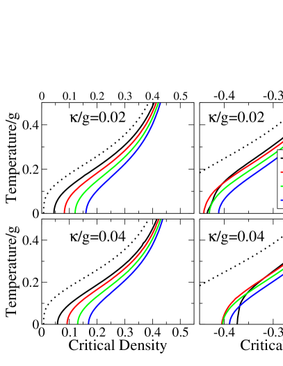
Figure 9: (Color online) Critical density (and associated critical bath chemical potential) at a given non-zero bath temperature. Evaluated for a Gaussian density of states, with $\sigma_{\epsilon}=0.15g$ and values of $\kappa$ and $\gamma$ as indicated in the legend. The dotted line marks the limit $\kappa\to 0$, $\gamma\to 0$, for which the equilibrium result, with distributions set by the pumping bath is recovered.

It is apparent that the presence of pumping and decay shifts the phase boundary to higher densities, and that the $\rho\to 0$ as $T\to 0$ behaviour seen in equilibrium does not survive. Physically, this increase of critical density is due to the decoherence introduced by pumping and decay. The behaviour at $T\to 0$ is unsurprising, as the limit $\rho\to 0$ corresponds to the equilibrium chemical potential $\mu\to-\infty$. In the presence of non-zero decay rate $\kappa$, one requires a non-zero effective gain (imaginary part of gap equation), and so no solution exists with $\mu_{B}\to-\infty$ even at $T=0$, i.e the critical density never goes to zero.

VII Fluctuations in condensed state to all orders in phase

The low energy modes of the broken symmetry system correspond to slow phase variations. Since there is no cost to global phase rotations, the action depends only on derivatives of the phase, and so phase fluctuations may become large. Thus, describing $\psi=\psi_{0}+\delta\psi$ and considering only terms to second order in $\delta\psi$ may underestimate how phase fluctuations reduce long range coherence. Therefore, we will instead consider the parameterisation $\psi=\sqrt{\rho_{0}+\pi}e^{i\phi}$, and evaluate correlation functions of $\psi$ in terms of the correlation functions of amplitude $\pi$ and phase $\phi$, including the phase fluctuations to all orders. In equilibrium, the effect of phase fluctuations on the field-field correlator is responsible for the reduction from long range order to power law correlations in two dimensions, and so has been much studied (see e.g. Refs. Nagaosa, ; Popov, ). Here, in order to calculate the luminescence and absorption spectrum, we will however need also to include density fluctuations.

Combining such a reparameterisation of the fields with the non-equilibrium Keldysh formalism requires a little care. The first important consideration is that the parameterisation requires one to work with fields where $\langle|\psi|^{2}\rangle$ is macroscopic. This means we should re-parameterise the fields $\psi_{f},\psi_{b}$ defined on the forward and backward contour (see Sec. III), as opposed to the fields $\psi_{q},\psi_{cl}$, since $\langle|\psi_{q}|^{2}\rangle$ is not macroscopic. This consideration is similar to the fact that the parameterisation should be done for the fields as functions of space and time rather than functions of ${\mathbf{p}}$ and $\omega$. The second consideration is that, in calculating the physical correlation functions, ${\cal D}^{<,>}$, this will involve cross terms between the two branches, and so one must keep track of which branch $\pi$ and $\phi$ are on.

The technical details of how to derive the field-field correlation functions in terms of amplitude and phase Green’s functions are presented in Appendix B. For the forward Green’s function (corresponding to luminescence), the result is found to be:

$$i\mathcal{D}^{<}_{\psi^{\dagger}\psi}(t,r)=\rho_{0}\left\{1+\frac{i}{2\rho_{0}}\left[i\mathcal{D}^{<}_{\phi\pi}(t,r)-i\mathcal{D}^{<}_{\pi\phi}(t,r)\right]\right.\\ -\frac{1}{4\rho_{0}^{2}}\left[i\mathcal{D}^{<}_{\pi\pi}(0,0)-i\mathcal{D}^{<}_{\pi\pi}(t,r)\vphantom{\mathcal{D}^{<}_{\phi}}\right]\\ +\frac{1}{8\rho_{0}^{2}}\left[i\mathcal{D}^{<}_{\phi\pi}(0,0)+i\mathcal{D}^{<}_{\pi\phi}(0,0)-i\mathcal{D}^{<}_{\phi\pi}(t,r)-i\mathcal{D}^{<}_{\pi\phi}(t,r)\right]^{2}\\ \left.\vphantom{\frac{1}{8}}\right\}\exp\left\{-\left[i\mathcal{D}^{<}_{\phi\phi}(0,0)-i\mathcal{D}^{<}_{\phi\phi}(t,r)\right]\right\}$$ (34)

The above procedure includes amplitude fluctuations $\pi$ and gradients of phase fluctuations $\nabla\phi,\partial_{t}\phi$ to second order as they both have restoring force, and cost energy, so that they are expected to be small. The phase fluctuations $\phi$ however may be large and in the above result are taken to all orders.

To calculate the luminescence spectrum one must then Fourier transform the result ${\cal D}^{<}_{\psi^{\dagger}\psi}(t,r)$ to give the spectrum in frequency and momentum space. The first term in the braces in Eq. (34) proportional to $\rho_{0}$ describes the emission from the condensate which is now broadened by the exponential term containing the phase fluctuations. It is clear that the phase fluctuations determine the condensate lineshape and the decay of spatial and temporal coherence. An example of luminescence as given by Eq. (34) is shown in Fig. 10. We will discuss its features in Section VII.1.

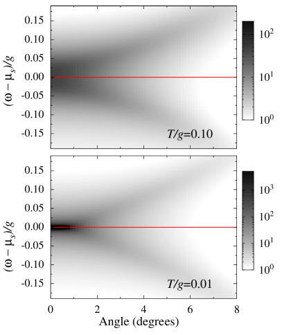
Figure 10: (Color online) Photoluminescence from the region of small $\omega$ and small $p$ (shown it terms of an angle of emission $\theta=\tan^{-1}(cp/\omega_{0})$, calculated including effects of phase fluctuations to all orders. Both panels have $\kappa=0.02g,\gamma=0.2g,\mu_{B}=0.0g$. The upper panel has $T=0.1g$ as in the middle row of Fig. 11, while the lower has $T=0.01g$, for which the features described in the text appear more sharply.

If one were to assume phase fluctuations were small, then this expression could be expanded to linear order in Green’s functions, and one would find:

$$i\mathcal{D}^{<}_{\psi^{\dagger}\psi}(t,r)=\rho_{0}\left\{1-\frac{i\mathcal{D}^{<}_{\pi\pi}(0,0)}{4\rho_{0}^{2}}-i\mathcal{D}^{<}_{\phi\phi}(0,0)\right\}\\ +\frac{i\mathcal{D}^{<}_{\pi\pi}(t,r)}{4\rho_{0}}+\frac{i}{2}\left(i\mathcal{D}^{<}_{\phi\pi}(t,r)-i\mathcal{D}^{<}_{\pi\phi}(t,r)\right)+\rho_{0}i\mathcal{D}^{<}_{\phi\phi}(t,r)$$

This is instructive, as the second line describes the fluctuation Green’s function $i\mathcal{D}^{<}_{\delta\psi^{\dagger}\delta\psi}(t,r)$, obtained taking the fluctuation fields to second order, while the first corresponds to a depleted condensate density. Such a linearisation would describe the luminescence as a sum of two terms; a condensate term, which due to its lack of space or time dependence would be a sharp peak, and a fluctuation term. Furthermore, if one were to consider the frequency spectrum of fluctuations by integrating this linearised form over momentum one would have a simple power law form, with a power depending only on the dimensionStaliunas , and not on parameters of the system.

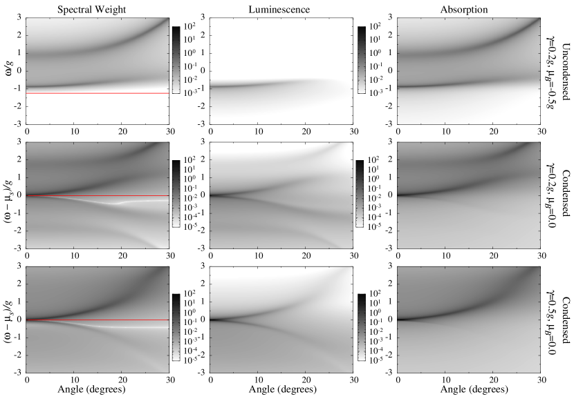
Figure 11: (Color online) Spectral weight, photoluminescence and absorption spectra, as a function of emission angle, $\tan^{-1}(cp/\omega_{0})$. For all graphs, $\kappa=0.02g$ and $T=0.1g$. Top row: Uncondensed case, $\gamma=0.2g,\mu_{B}=-0.5g$. (cf parameters in Fig. 3 and Fig. 4) Middle row: Condensed case, $\gamma=0.2g,\mu_{B}=0.0g$. Bottom row: Condensed case, $\gamma=0.5g,\mu_{B}=0.0g$ (transition to weak coupling).

By allowing phase fluctuations to be large, and keeping the phase-phase Green’s function in the exponent, the condensate acquires a lineshape as a result of phase fluctuations, and this lineshape can in the equilibrium limit recover the standard power law correlations seen in two dimensions. The form of this lineshape is discussed further in Sec. VII.1.

However, for $\omega,p$ far from zero, such linearisation does not introduce any major changes; the effects of large phase fluctuations matter mostly at large times. Large fluctuations between fields separated by small $t$ or $r$ would imply large gradients, and thus have a large energy cost. Thus, Fig. 11 illustrates the absorption, luminescence and spectral weight over large ranges of $\omega,p$ using a linearised approach [which at this large scale coincides with the full expression given by Eq. (34)] while Fig. 10, obtained from the full expression of Eq. (34), shows the effect of phase fluctuations at small $\omega,p$.

For the detailed analysis of the features of the luminescence spectra we refer to Ref. keldysh_letter, . Note that for large $\omega,p$ as shown in Fig. 11 the main features of the non-equilibrium spectra are similar to those predicted for equilibrium condensation in Refs. Keeling, ; Marchetti, . In the normal state one can see the upper and lower polariton modes (top row of Fig. 11) in the spectral weight and absorption, and only the lower polariton in the luminescence as the upper polariton is not occupied at this low power. When system condenses (middle row of Fig. 11) the structure of modes changes dramatically showing the pairs of phase and amplitude modes above and below the chemical potential. Finally, when the coupling to the pump baths; i.e. the pumping strength is further increased (bottom row of Fig. 11) the system crosses to weak-coupling regime and the polariton splitting is suppressed. In Fig. 11 the occupation of the excited states will not be thermal, in contrast to the analogous figures in Refs. Keeling, ; Marchetti, , this is however not easy to observe on these contour plots. Also since Fig. 11 corresponds to pumping baths at finite temperature in contrast to zero temperature in Ref. keldysh_letter, the sharp occupation edge visible there is here smeared out. However the main qualitative difference between the spectra of a pumped decaying condensate presented here and that for a closed system given in Refs. Keeling, ; Marchetti, is most visible on small $\omega,p$ scale as presented in Fig. 10. This will be discussed in detail in the Section VII.1.

VII.1 Condensate Lineshape - effects of dissipation and low-dimensionality on decay of correlations

The long range field-field correlations are influenced by the properties of the soft phase modes; i.e. the Goldstone or Bogoliubov modesWouters05 ; keldysh_letter . By considering the asymptotic behaviour of the phase-phase correlator at small frequencies and momenta, one can thus find the asymptotic form of the field-field correlator. In an equilibrium two-dimensional system, the long distance field-field correlations decay with a power law below the BKT transition. We will now investigate how this asymptotic behaviour is affected by the presence of pump and decay. For convenience let us rewrite Eq. (50), assuming an isotropic system:

$$i\mathcal{D}^{<}_{\psi^{\dagger}\psi}(t,r) =\rho_{0}\left[1+\mathcal{O}\left(1/\rho_{0}\right)\right]\exp\left[-f(t,r)\right],$$ (35)

$$f(t,r) =\int\frac{d\omega}{2\pi}\int\frac{pdp}{2\pi}\left[1-J_{0}(pr)e^{i\omega t}\right]i\mathcal{D}^{<}_{\phi\phi}(\omega,p).$$ (36)

Here $J_{0}(pr)$ is a Bessel function, from the integration over azimuthal angle. We are thus interested in the limits $f(t=0,r\to\infty)$ and $f(t\to\infty,r=0)$, describing the large distance and long time decay.

For comparison, let us first summarise how this method reproduces the standard result in the equilibrium case. In equilibrium, the distribution function is a constant matrix $F(\omega)=2n_{B}(\omega)+1$, and so:

$$i\mathcal{D}^{<}_{\phi\phi}(\omega,p) =\frac{1}{2}\left(F(\omega)-1\right)\left(i\mathcal{D}^{R}_{\phi\phi}(\omega,p)-i\mathcal{D}^{A}_{\phi\phi}(\omega,p)\right)$$

$$=n_{B}(\omega)(-2)\mathrm{Im}\left[\mathcal{D}^{R}_{\phi\phi}(\omega,p)\right]$$ (37)

For an equilibrium coherent system, the low energy modes will be the linear Goldstone modes of the form $\omega=cp$. By analytic continuation of the imaginary time (Matsubara) Green’s function, one finds:

$$\mathrm{Im}\left[\mathcal{D}^{R}_{\phi\phi}(\omega,p)\right] =\mathrm{Im}\left[\frac{-C}{(\omega+i0^{+})^{2}-c^{2}p^{2}}\right]$$

$$=-\frac{\pi C}{2cp}\left(\delta(\omega-cp)-\delta(\omega+cp)\right)$$ (38)

And so, combining Eq. (36), Eq. (37) and Eq. (38) one finds that the singular contribution to $f(t,r)$ is given by:

$$f(t,r)=\frac{C}{2\pi\beta c}\int_{0}^{1/\beta c}\frac{dp}{p}\left[1-J_{0}(pr)\cos(cpt)\right]+\ldots,$$ (39)

where $\beta$ is inverse temperature, and the effect of the thermal distribution has been approximated by the upper cutoff of the integral. The lower cutoff is controlled by how $J_{0}(pr)\cos(cpt)$ approaches $1$ as $p\to 0$, and thus depend on $r$ and $ct$. For small $p$, the leading term in the expansion for both $\cos(cpt)$ and $J_{0}(pr)$ is quadratic, and so the lower cutoff for the integral is given by $p\simeq 1/\sqrt{r^{2}+c^{2}t^{2}}$. Thus,

$$f(t,r)\simeq\eta\ln\left(\frac{\sqrt{c^{2}t^{2}+r^{2}}}{\beta c}\right).$$

Thus, one recovers the standard result, and logarithmic behaviour of $f(t,r)$ leads to power decay of correlation functions, with $\eta\propto k_{B}T/\rho_{0}$. One can further use this result to find the form of the peak in the luminescence spectrum, $\mathcal{L}(\omega,p)\propto(c^{2}p^{2}+\omega^{2})^{(\eta-3)/2}$, and the integrated luminescence (i.e. angular profileKeeling ) $N(p)\propto p^{\eta-2}$.

Let us now consider the asymptotic form of the Green’s function in the non-equilibrium case. We shall first consider the retarded Green’s function, as the poles of this function describe the normal modes; the result of calculating $\mathcal{D}_{\phi\phi}^{<}$ will, as discussed later, be to introduce the population of these modes. The retarded Green’s function, using the notation of Eq. (21) can be written as:

$$i\mathcal{D}^{R}_{\phi\phi}(\omega,p)=\frac{C}{K_{1}^{R}(\omega,p)K_{1}^{R}(-\omega,p)-K_{2}^{R}(\omega)K_{2}^{R}(\omega)}$$

As discussed in Sec. V.3, the gap equation implies that $K_{1}^{R}(\omega=0,p=0)=K_{2}^{R}(\omega=0)$. Combining this with the symmetries in Eq. (22), one can show that the most general expression, to quadratic order in $p,\omega$ in the denominator can be written as:

$$\mathcal{D}_{\phi\phi}^{R}(\omega,p)\simeq\frac{C}{\omega^{2}-c^{2}p^{2}+2i\omega x},$$ (40)

where $C,c$ and $x$ are coefficients to be derived from the full expressions. Without pumping and decay, $x=0^{+}$, and one recovers the equilibrium result. With non-zero $x$, the poles of the Green’s function, which define the low energy modes of the system, have the form

$$\omega=-ix\pm i\sqrt{x^{2}-c^{2}p^{2}},$$

and are thus diffusive, rather than dispersive for $p\leq x/c$keldysh_letter . This can be clearly seen in the luminescence shown in Fig 10: At low momentum, where the real part of the pole vanishes, but the imaginary part does not, the luminescence is dispersionless (i.e. flat), but broadened. Such a form should be generic for broken symmetry in a pumped decaying system, and indeed the same form has been recently seen in a related context, of coherently pumped polaritons in photonic wires, described as an optical parametric oscillatorWouters05 , as well as in a more generic modelWouters07 . This result also shows why it was so important to have solved a complex gap equation, rather than just adding decay rates to the equilibrium model. Adding phenomenological decay rates “by hand” would lead to a form of the retarded Green’s function:

$$\mathcal{D}^{R}_{\phi\phi}(\omega,p)=\frac{C}{(\omega+ix)^{2}-c^{2}p^{2}}$$

Such a form does not describe a system with spontaneously broken symmetry, as there is no pole at $\omega=0,p=0$, and thus such an approach misses the appearance of a diffusive mode.

Let us now consider ${\cal D}^{<}_{\phi\phi}$, and thus the effect of the distribution function. As was discussed in Sec. V.1, the distribution function can be expected to diverge at the energy where the imaginary part of the denominator of the retarded Green’s function vanishes. This is clear at $\omega=0$ (measured relative to the common oscillation frequency $\mu_{S}$), due to the presence of a real pole at $\omega=0,p=0$. However, this divergence will be exactly canceled by the vanishing of $\mathcal{D}^{R}(\omega,p)-\mathcal{D}^{A}(\omega,p)$ as $\omega\to 0$, since both the divergence and the vanishing are due to the same imaginary part. Thus, near $\omega=0$, the asymptotic form of $\mathcal{D}^{<}_{\phi\phi}(\omega,p)$ is the same as that of $|\mathcal{D}^{R}_{\phi\phi}(\omega,p)|^{2}$, i.e.:

$$i\mathcal{D}^{<}_{\phi\phi}(\omega,p)\simeq\frac{C^{2}}{(\omega^{2}-c^{2}p^{2})^{2}+4\omega^{2}x^{2}}.$$

The effect of the distribution will be to introduce some upper energy cutoff. Thus, the equivalent of Eq. (39) is:

$$f(t,r)=\frac{\pi C}{2c^{2}x}\int_{0}^{1/\xi_{c}}\frac{dp}{p}\left[1-J_{0}(pr)d(p,t)\right]$$ (41)

where the time dependence is described by:

$$d(p,t)=e^{-xt}\left[\frac{x}{\sqrt{x^{2}-c^{2}p^{2}}}\sinh\left(\sqrt{x^{2}-c^{2}p^{2}}t\right)\right.\\ \left.+\vphantom{\frac{x}{\sqrt{x^{2}-c^{2}p^{2}}}}\cosh\left(\sqrt{x^{2}-c^{2}p^{2}}t\right)\right]$$ (42)

Equation (41) has a similar interpretation to Eq. (39), a large $p$ cutoff from the distribution function and a short distance cutoff set by the coordinates. For a thermal distribution function, the upper cutoff would be given by $1/\xi_{c}\simeq k_{B}T/c$. Although the photon distribution in the pumped decaying system is not thermal, if the pumping and decay baths are thermal (as considered earlier), then the photon distribution will vanish for large enough energies. As such, we will write $1/\xi_{c}\simeq E_{\mathrm{max}}/c$, where $E_{\mathrm{max}}$ depends on both pumping and decay, and would reduce to $k_{B}T$ in equilibrium. The result is thus $f(t,r)\simeq\eta^{\prime}\ln(1/Q\xi_{c})$, where $Q$ is the lower cutoff. However, the form of the lower cutoff can be different, and depends on the relative values of $r$, $ct$ and $c/x$. In the two regions of interest defined at the start of this section, one finds:

$$Q=\begin{cases}\frac{1}{c\sqrt{t/x}}&\text{if $r\simeq 0$, $t\to\infty$,}\\ \frac{1}{r}&\text{if $r\to\infty$, $t\simeq 0$.}\end{cases}$$ (43)

Inserting this cutoff, one finds

$$f(t,r)\simeq\begin{cases}(\eta^{\prime}/2)\ln(c^{2}t/x\xi_{c}^{2})&\text{if $r\simeq 0$, $t\to\infty$,}\\ \eta^{\prime}\ln(r/\xi_{c})&\text{if $r\to\infty$, $t\simeq 0$.}\end{cases}$$ (44)

Thus, there is still power law decay, but due to pumping and decay the powers for temporal and spatial decay do not match, and since $\eta^{\prime}$ may depend on $x$, both power laws will differ from equilibrium.

Since the long time decay is power law, the lineshape will also have a power law divergence at low frequency, and as such there is no well defined condensate linewidth in an infinite system. In fewer than two dimensions, i.e. in a 1D systemWouters05 , or a fully confined system such as a laser with discrete modes, the long time decay will be exponential, and so a linewidth can be found in such systems. The crossover between power law and exponential decay in a large but finite 2D system is discussed in Sec. VIII. In three dimensions, the limit of $f(t,r)$ at large times and distances is finite (as opposed to divergent as in two, one or zero dimensions). As a result, there is phase coherence to arbitrarily large distances, and so, writing the asymptotic values of $f(t,r)$ as $f_{\infty}$ there is a contribution to the luminescence that goes like:

$$i\mathcal{D}^{<}_{\psi^{\dagger}\psi}(\omega,{\mathbf{p}}) =\int dt\int d^{3}{\mathbf{r}}\rho_{0}e^{-f_{\infty}}e^{i\omega t+i{\mathbf{p}}\cdot{\mathbf{r}}}+\ldots$$

$$=\rho_{0}e^{-f_{\infty}}\delta(\omega)\delta^{3}({\mathbf{p}})+\ldots,$$

i.e., in an infinite homogeneous $3D$ system, there would be a peak at $\omega=0,{\mathbf{p}}=0$, with a peak height given by the condensate density, which is depleted by phase fluctuations.

VIII Finite size effects

In the previous section we discussed how the continuum of phase modes leads, in two dimensions, to logarithmic phase-phase correlation functions as a function of distance and time. In this section, we consider how confinement, which leads to a discrete spectrum of phase modes will modify that result. In a confined system, there will not be translational invariance, and so the field-field correlation function will in general depend on both positions, rather than just on separation. However, if we are interested in the equal-position, long-time limit, which is relevant for the lineshape, we can then write:

$$f(t,r,r)=-\sum_{n}\int\frac{d\omega}{2\pi}\frac{C|\varphi_{n}(r)|^{2}(1-e^{i\omega t})}{(\omega^{2}-\zeta_{n}^{2})^{2}+4\omega^{2}x^{2}},$$

where we have introduced the wavefunction $\varphi_{n}(r)$ and energy $\zeta_{n}$ of the $n^{\mathrm{th}}$ phase mode. It is clear that if $\varphi_{n}(r)=e^{ip_{n}r}$, and $\zeta_{n}=cp_{n}$, we recover the previous result.

Let us now discuss briefly the energy spacing $\Delta$ of phase modes $\zeta_{n}$. Schematically, for a box of size $R$, one has $\Delta=c/R$, i.e. the sound modes, with discrete momentum spacing. In contrast, the energy spacing of single particle states in such a box would be $\delta=1/2mR^{2}$. Since the sound velocity increases as condensate density increases, one can have $\Delta\gg\delta$. [NB in a harmonic trap, the Thomas-Fermi radius and the sound velocity have the same dependence on $\rho_{0}$, so the phase mode level spacing is the single particle spacingStringari96 . A harmonic trap is however a special case in this regard.]

To understand how discrete mode spacing modifies $f(t,r,r)$, let us first reconsider how the logarithm term arose from the integral. Schematically, we had:

$$f(t,r,r)\simeq\int_{0}^{Q}\frac{dp}{Q}+\int_{Q}^{1/\xi_{c}}\frac{dp}{p}=\frac{Q}{Q}+\ln\left(\frac{1}{\xi_{c}Q}\right)$$

i.e., the dependence on the coordinates, via the cutoff $Q$ is logarithmic, as the contribution from $p\leq Q$ is constant. For the discrete sum, after integrating over $\omega$, instead of Eq. (41) we have:

$$f(t,r,r)=\frac{\pi C}{2x}\sum_{n}^{N}\frac{|\varphi_{n}(r)|^{2}}{\zeta_{n}^{2}}\left[1-d\left(p=\frac{\zeta_{n}}{c},t\right)\right]$$ (45)

with $d(p,t)$ as in Eq. (42). The upper cutoff is introduced here by truncating the sum at $N$ such that $\zeta_{N}=c/\xi_{c}\simeq E_{\mathrm{max}}$. Considering the long time limit, this sum can also be split into two parts; for modes $\zeta_{n}\ll 1\sqrt{x/t}$ the summand is effective energy independent, while for $\zeta_{n}\gg\sqrt{x/t}$, with the density of states in 2D, one recovers a log divergence. However, the existence of these two parts depends on the relative values of the energy of the lower cutoff $\sqrt{x/t}$, the upper cutoff $E_{\mathrm{max}}$, and the level spacing $\Delta$. We assume $E_{\mathrm{max}}\gg\sqrt{x/t}$, which just means considering long enough time delays, and so there are three important cases:

1. $\Delta\ll\sqrt{x/t}\ll E_{\mathrm{max}}$. In this case there are many terms contributing to both the small and large $\zeta_{n}$ sums, and so the the result is as for the integral: schematically $f(t,r,r)=1+\ln(E_{\mathrm{max}}\sqrt{t/x})$, and there are power laws, as in the infinite system. This case cannot however persist to arbitrarily large times.

2. $\sqrt{x/t}\leq\Delta\ll E_{\mathrm{max}}$. At long enough times, the previous case will switch to this case. Here, there are only a few terms in the low energy contribution. A characteristic term, for $\zeta_{n}\ll x$ gives $d(\zeta_{n}/c,t)\simeq 1-\zeta_{n}^{2}t/2x$. Since the number of low energy modes is now of order $1$, rather than of order $x/t\Delta^{2}$, the contribution from these modes is of order $t/x$, and not of order 1. Thus, the dominant contribution is $f(t,r,r)\simeq(\pi C/2x)(t/2x)$, and so the decay of field-field correlations is exponential as in a single mode case.

3. $\sqrt{x/t}\ll E_{\mathrm{max}}\ll\Delta$. In this case, no phase fluctuations are populated, i.e. no terms survive in the sum, and so the entire system is coherent. Using $\Delta=c/R$, this condition is equivalently $R\ll\xi_{c}=c/E_{\mathrm{max}}$, i.e. the “thermal length” is larger than the system sizePetrov00 .

To summarise, if temperature is low enough (or in the case of non-thermal distribution the relevant energy to which the modes are occupied is small enough), phase fluctuations are frozen out, as one expects. If phase fluctuations are not frozen out, there are two limits; at long enough times, one always sees linear growth of fluctuations, resulting in the exponential decay of field-field correlations, and recovery of the standard laser lineshapeHaken:Laser . However, for large enough systems, so level spacing is small, there is a range of time delays during which the growth of phase fluctuations is logarithmic in time, giving rise to a power-law decay of field-field correlations, as one would expect in the infinite system.

VIII.1 Self-phase modulation

The analysis so far shows how, due to finite size, the power law correlations associated with a continuum of modes change to the exponential decay of correlations associated with phase diffusion of a single mode. There has been previous work on extending the picture of phase diffusion of a single mode due to pumping noiseHaken:Laser to the case of interacting systems, for which there is an additional source of noise from self-phase modulation (SPM)Holland96 ; Tassone00 ; Porras03 . These works suggest that the phase decay rate can be written as $x\simeq(\Gamma_{0}+\rho_{0}^{2}X_{\text{spm}})/\rho_{0}$, where $\Gamma_{0}$ is the noise due to pumping, $\rho_{0}$ the condensate density, and $X_{\text{spm}}$ proportional to interaction strength. We wish here to comment briefly on the origin of the SPM term, and how it may be modified in the case of many interacting modes, with respect to the case of phase diffusion of a single mode.

The presence of a SPM term can be understood by considering the evolution of a coherent state, $e^{\sqrt{\rho_{0}}\psi^{\dagger}}|0\rangle=\sum_{n}(\sqrt{\rho^{n}/n!})|n\rangle$. For an interacting single mode system, the number states are eigenstates, and have energies like $E_{n}=an+bn^{2}$, thus different number states evolve at different frequencies, and mutually dephase, leading to a dephasing rate $x_{\text{spm}}\simeq b\rho_{0}$. Thus, SPM occurs because number states, not coherent states are eigenstates of the single mode Hamiltonian. The eigenstates of the many mode system, including coherent interactions between modes, such as $\psi^{\dagger}_{0}\psi^{\dagger}_{0}\psi^{\vphantom{\dagger}}_{p}\psi^{\vphantom{\dagger}}_{-p}$ are neither number states nor coherent states, but are instead better described by Noizérres-Bogoliubov statesNozieres82 . Such states are superpositions of terms with different divisions of particles between the condensate and non-condensed modes; while they may be eigenstates of total number, they are not eigenstates of the number of particles in a given mode, and they lower energy because of the coherence between the different modesLittlewood04 . As such, when considering systems with a continuum of interacting modes, it is not clear that SPM terms should exist, or if they exist, should have the same form.

IX Conclusions

In conclusion, we have studied steady-state spontaneous quantum condensation in a non-equilibrium Bose-Fermi system with pumping and decay, and consequent flux of particles. In order to study the effect of large phase fluctuations in the broken symmetry system, it was necessary to extend the path-integral Keldysh formalism to deal with a reparameterisation in terms of phase and amplitude fluctuations, for fields on the forward and backward time contours. We have shown that the mean-field properties of a pumped and decaying condensate can be described by a complex analogue of the Gross-Pitaevskii equation in the BEC regime (or equivalently the gap equation in the BCS regime). The real part of this self-consistency equation relates the coherent field to the system’s non-linear susceptibility as in the case of equilibrium condensation, while the imaginary part reflects how the gain and decay are balanced, as in a laser. We further show that it is crucial to satisfy this complex self-consistent equation in order to get the correct collective mode structure, reflecting the broken symmetry.

We have analysed the solutions of this complex gap equation and examined their stability. Surprisingly, despite non-thermal distributions, the instability of the normal state is analogous to that in thermal equilibrium, where the normal state becomes unstable when the chemical potential, at which the Bose-Einstein distribution diverges, reaches the bottom of the system’s spectrum. In the non-equilibrium case, the system’s distribution, although far from thermal, develops a divergence at some energy. When, by tuning parameters of the system, this energy is brought to coincide with an effective pole of the system’s Green’s function, then the normal state becomes dynamically unstable and the condensation transition takes place. We have also shown that whenever there is a condensed solution, the normal state becomes dynamically unstable, and so there is no ambiguity as to which state the system would choose. However, we have found a range of parameters where both the normal and the uniform harmonic condensed solutions are unstable, suggesting either more exotic, perhaps chaotic, dynamics or spatial pattern formation.

We have analysed the non-equilibrium phase diagram as a function of the decay and pump parameters, and have found both the low density condensed solutions when pump and decay strengths are relatively small, as well as the high density, inverted, laser-like solutions when pump and decay are comparable to the inter particle interactions. When applied to microcavity polaritons these regimes reflect the spontaneous condensation of strongly coupled photon-exciton modes at relatively small pump and decay powers, and the crossover to the weak-coupling regime and the photon laser at large pump powers. It is important to stress that even if the system distribution is close to thermal the presence of pump and decay, i.e. particle flux, result in a higher critical density at a given temperature than in a closed system, and there is a non-zero minimum critical density even at zero temperature.

Having analysed the fluctuation spectra and collective modes, we have found an important difference between condensation in a dissipative environment and that in closed systems: Although there is a real pole (undamped mode) at zero frequency and momentum, indicating broken symmetry, the usual linear dispersion of the sound mode (Bogoliubov, Goldstone mode) at small momenta is now replaced by diffusive behaviour (i.e. a broadened but flat dispersion); this questions the possibility of superfluidity on large time and distance scales. This qualitatively new structure of the collective modes is visible in the luminescence and absorption spectra, and it affects the field-field correlations, i.e. decay of spatial and temporal coherence, and the condensate lineshape. For example, in the 2D system dissipation changes the usual power-law decay of spatial and temporal coherence, replacing it by one where the powers for temporal and spatial decay do not match.

It is instructive to place our treatment of non-equilibrium quantum condensation in the context of other works on dynamic effects in polariton systems. Much of the literature concentrates on Boltzmann-like rate equations. Such an approach allows one to study the effect of pumping and decay on the occupation of modes;Tassone97 ; Porras02 ; savaona06 but is not able to account for the changes to the excitation spectrum and the density of states (which are particularly dramatic as the system crosses the phase transition) due to the pumping, decay and presence of the coherent field. In contrast, field theoretical studies presented here selfconsistently account both for arbitrarily large changes to the excitation spectrum as well as changes to the occupation of this spectrum. Such approaches are thus well placed to study the phase transition between the non-condensed and condensed states, and in addition the crossover between strong and weak coupling regimes. A closer approach to the field-theoretical approach presented here would be the evolution of the off diagonal parts of the full density matrixPorras03 ; Laussy04 . It was however only recently that qualitative changes to the spectrum have been calculated using the density matrix approach (in the context of parametric emission from photonic wires) in Refs. Wouters05, ; Wouters06, . A further distinction is between single-mode models, in which one expects phase diffusion (e.g. Refs. Porras02, ; Tassone00, ) and exponential decay of correlations as in lasers, and models with a continuum of modes, such as Refs. keldysh_letter, ; Wouters05, ; Wouters06, and this paper.

Finally, in this paper we have analysed how the finite size of the system affects the decay of temporal coherence. This is particularly important for the understanding of recent experimentsKasprzak06 , as well as for providing a connection to similar analysis for single mode photon lasers, which are still used as the basis to describe the decay of coherence in atom and polariton lasers. The key difference between the output from the condensate and from a single mode laser is that in the condensate there is a continuum of modes, and so spatial fluctuations play an important role — in 2D they destroy the long-range order and lead to a power-law decay of correlations. Including such spatial fluctuations, the growth of phase fluctuations as a function of time is logarithmic, which gives power-law decay of temporal coherence, rather than the exponential decay expected for a single mode. In single mode systems such as the laser, there are no spatial fluctuations, and so the decay of coherence is determined entirely from the phase diffusion of this single mode. However, if one takes a continuum system, and reduces its size, the energy spacing of modes becomes larger, and so the number of modes whose energies are low enough to be relevant decreases, eventually recovering the single mode limit. We have identified two regimes in the finite system: Where the level spacing is larger than temperature, and so spatial fluctuations are essentially frozen out, resulting in an exponential decay of correlations as in a single mode laser; and where the level spacing is small with respect to temperature, so one gets a power-law decay of temporal coherence at short times as in the infinite system, crossing over to exponential decay at larger times.

The qualitative implications of our results are general, and can apply to any BEC or BCS condensate which is subject to dissipation. The immediate applications of this analysis are for polariton BEC, which are naturally faced with significant pumping and decay processes. However, the techniques and results developed here, can be of use in understanding a wider class of broken symmetry dissipative systems; for example resonant parametric oscillators, and atom lasers, where coherence, dephasing, and the interaction of many modes are all relevant.

Appendix A Gap equation at T=0

In the limit of $T=0$, the integrals in the gap equation, Eq. (15) can be evaluated in terms of elementary functions. This makes numerical analysis of the equations much easier in this limit. The results of this analysis are presented in Sec. VI; for completeness we show the explicit expressions at $T=0$ here. At $T=0$, the bath distributions take a simple form $F_{b}(\omega)=\rm{sign}(\omega-\tilde{\mu}_{B})$ and $F_{a}(\omega)=\rm{sign}(\omega+\tilde{\mu}_{B})$ and so the real and the imaginary parts of the gap equation become:

$$\tilde{\omega}_{0}=-\frac{g^{2}\gamma\tilde{\epsilon}}{2\pi 2E(E^{2}+\gamma^{2})}\rm{ln}\frac{(E+\mu_{B}-\frac{\mu_{S}}{2})^{2}+\gamma^{2}}{(E-\mu_{B}+\frac{\mu_{S}}{2})^{2}+\gamma^{2}}+\\ \frac{g^{2}}{2\pi E}\left(\rm{ArcTan}\frac{E+\mu_{B}-\frac{\mu_{S}}{2}}{\gamma}+\rm{ArcTan}\frac{E-\mu_{B}+\frac{\mu_{S}}{2}}{\gamma}\right)-\\ \frac{g^{2}\tilde{\epsilon}}{2\pi(E^{2}+\gamma^{2})}\left(\rm{ArcTan}\frac{E+\mu_{B}-\frac{\mu_{S}}{2}}{\gamma}\right.-\\ \left.\rm{ArcTan}\frac{E-\mu_{B}+\frac{\mu_{S}}{2}}{\gamma}\right),$$

and

$$\frac{\kappa}{\gamma}=\frac{g^{2}\gamma}{2\pi 2E(E^{2}+\gamma^{2})}\rm{ln}\frac{(E+\mu_{B}-\frac{\mu_{S}}{2})^{2}+\gamma^{2}}{(E-\mu_{B}+\frac{\mu_{S}}{2})^{2}+\gamma^{2}}+\\ \frac{g^{2}}{2\pi(E^{2}+\gamma^{2})}\left(\rm{ArcTan}\frac{E+\mu_{B}-\frac{\mu_{S}}{2}}{\gamma}\right.-\\ \left.\rm{ArcTan}\frac{E-\mu_{B}+\frac{\mu_{S}}{2}}{\gamma}\right).$$

The expression for fermion-pair (exciton) density (16) at $T=0$ reduces to:

$$\frac{1}{2}\left(b^{\dagger}b-a^{\dagger}a\right)=\frac{g^{2}\gamma|\psi_{f}|^{2}}{4\pi E(E^{2}+\gamma^{2})}\rm{ln}\frac{(E-\mu_{B}+\frac{\mu_{S}}{2})^{2}+\gamma^{2}}{(E+\mu_{B}-\frac{\mu_{S}}{2})^{2}+\gamma^{2}}\\ -\frac{\tilde{\epsilon}}{2\pi E}\left(\rm{ArcTan}\frac{E-\mu_{B}+\frac{\mu_{S}}{2}}{\gamma}+\rm{ArcTan}\frac{E+\mu_{B}-\frac{\mu_{S}}{2}}{\gamma}\right)\\ +\left(\frac{g^{2}|\psi_{f}|^{2}}{2\pi(E^{2}+\gamma^{2})}-\frac{1}{2\pi}\right)\left(\rm{ArcTan}\frac{E-\mu_{B}+\frac{\mu_{S}}{2}}{\gamma}\right.-\\ \left.\rm{ArcTan}\frac{E+\mu_{B}-\frac{\mu_{S}}{2}}{\gamma}\right).$$

Appendix B Evaluation of field correlations in terms of amplitude and phase fluctuations

To illustrate the idea of using phase and amplitude fluctuations, we will first present the simpler case of ${\cal D}^{T,\tilde{T}}$, for which both fields are on the same branch, and so we may drop all labels identifying which branch or Green’s function ($T$ or $\tilde{T}$) we are considering. Then, writing $\pm$ for the time, and coordinate indices $(T\pm t/2,{\mathbf{R}}\pm{\mathbf{r}}/2)$, one may write:

$$i{\mathcal{D}}_{\psi^{\dagger}\psi} =\left<\psi^{\dagger}(+)\psi^{\vphantom{\dagger}}(-)\right>$$

$$=\left<\sqrt{(\rho_{0}+\pi(+))(\rho_{0}+\pi(-))}e^{-i(\phi(+)-\phi(-))}\right>$$

The square root may be expanded to second order in the density fluctuations (as density fluctuations, unlike phase fluctuations, have a restoring force), thus:

$$i{\mathcal{D}}_{\psi^{\dagger}\psi}\simeq\rho_{0}\left<\left[1+\left(\frac{\pi(+)+\pi(-)}{2\rho_{0}}\right)-\frac{\left(\pi(+)-\pi(-)\right)^{2}}{8\rho_{0}^{2}}\right]\exp\left[-i(\phi(+)-\phi(-))\right]\right>.$$

Introducing a current $J$, one may write the correlators in terms of a generating functional as:

$$i{\mathcal{D}}_{\psi^{\dagger}\psi}=\rho_{0}\left\{1+\sum_{\omega,p}\frac{1}{\rho_{0}}\cos\left(\frac{\omega t}{2}+\frac{{\mathbf{p}}\cdot{\mathbf{r}}}{2}\right)\frac{\delta}{\delta J_{\omega,p}}+\frac{1}{2\rho_{0}^{2}}\left[\sum_{\omega,p}\sin\left(\frac{\omega t}{2}+\frac{{\mathbf{p}}\cdot{\mathbf{r}}}{2}\right)\frac{\delta}{\delta J_{\omega,p}}\right]^{2}\right\}\\ \times\left.\left<\exp\left[\sum_{\omega,p}J_{\omega,p}\pi(\omega,p)+2\sin\left(\frac{\omega t}{2}+\frac{{\mathbf{p}}\cdot{\mathbf{r}}}{2}\right)\phi(\omega,p)\right]\right>\right|_{J=0}.$$

By integrating over the photon field, the generating functional, ${\cal Z}[J]=\langle\exp[\dots]\rangle$, can be expressed in terms of the correlators of amplitude and phase fluctuations. Defining

$${\mathbf{J}}(\omega,p)=\left(\begin{array}[]{c}J_{\omega,p}\\ 2\sin\left[\left({\omega t}+{{\mathbf{p}}\cdot{\mathbf{r}}}\right)/2\right]\end{array}\right)$$

one may then write

$${\cal Z}[J]=\exp\left[\frac{1}{2}\sum_{\omega,p}{\mathbf{J}}(-\omega,p)^{T}i\tilde{\mathcal{D}}(\omega,p){\mathbf{J}}(\omega,p)\right]$$ (46)

where

$$\tilde{{\mathcal{D}}}=\left(\begin{array}[]{ll}{\mathcal{D}}_{\pi\pi}&{\mathcal{D}}_{\pi\phi}\\ {\mathcal{D}}_{\phi\pi}&{\mathcal{D}}_{\phi\phi}\end{array}\right).$$

Note that we use the standard definition of Green’s functions so that $i{\mathcal{D}}_{ab}=\langle ab\rangle$.

To determine these correlators one may either recalculate the effective action by writing $\psi$ in terms of $\pi$ and $\phi$ and expanding to second order in $\pi$ and derivatives of $\phi$; or one may use the fact that at second order, the amplitude-phase variables can be considered as a linear transform of $\delta\psi$ and $\delta\bar{\psi}$, i.e.:

$$\left(\begin{array}[]{l}\pi\\ \phi\end{array}\right)=L\left(\begin{array}[]{l}\delta\psi^{\vphantom{\dagger}}\\ \delta\psi^{\dagger}\end{array}\right),\quad L=\frac{1}{2\sqrt{\rho_{0}}}\left(\begin{array}[]{cc}2\rho_{0}&2\rho_{0}\\ -i&i\end{array}\right).$$

Note that this rotation relates the effective action expressed in terms of these variables, and is not to be used in finding the final correlation functions $\mathcal{D}_{\psi^{\dagger}\psi}$. Thus, one can express the amplitude-phase Green’s functions in terms of the $\delta\psi,\delta\psi^{\dagger}$ Green’s functions as:

$$\tilde{\mathcal{D}}^{R/A/K}=L\mathcal{D}^{R/A/K}L^{\dagger}.$$ (47)

The $T,\tilde{T}$ Green’s functions can then be found from the retarded, advanced and Keldysh components by using Eq. (26) and:

$${\mathcal{D}}^{T,\tilde{T}}=\frac{1}{2}\left({\mathcal{D}}^{K}\pm\left[{\mathcal{D}}^{R}+{\mathcal{D}}^{A}\right]\right).$$ (48)

Thus, one may write the $T$ or $\tilde{T}$ field correlation function in terms of the phase and amplitude Green’s functions:

$$i{\mathcal{D}}_{\psi^{\dagger}\psi}=\rho_{0}\left\{\vphantom{\left(\sum_{\omega,p}\frac{1}{2}\right)}1-\sum_{\omega,p}\sin\left(\omega t+{\mathbf{p}}\cdot{\mathbf{r}}\right)\frac{i\mathcal{D}_{\phi\pi}(\omega,p)}{\rho_{0}}-\sum_{\omega,p}\left[1-\cos\left(\omega t+{\mathbf{p}}\cdot{\mathbf{r}}\right)\right]\frac{i\mathcal{D}_{\pi\pi}(\omega,p)}{4\rho_{0}^{2}}\right.\\ \left.+\frac{1}{2}\left(\sum_{\omega,p}\left[1-\cos\left(\omega t+{\mathbf{p}}\cdot{\mathbf{r}}\right)\right]\frac{i\mathcal{D}_{\phi\pi}(\omega,p)}{\rho_{0}}\right)^{2}\right\}\exp\left\{-\sum_{\omega,p}\left[1-\cos\left(\omega t+{\mathbf{p}}\cdot{\mathbf{r}}\right)\right]i\mathcal{D}_{\phi\phi}(\omega,p)\right\}.$$ (49)

We can now address how to generalise this calculation when the two fields are on different branches. We will consider the forward (luminescence) Green’s function; the backward (absorption) will follow by swapping labels. Thus, repeating the above discussion, but keeping subscripts on the fields one has:

$$i\mathcal{D}^{<}_{\psi^{\dagger}\psi}(t,r)=\rho_{0}\left<\left[1+\left(\frac{\pi_{b}(+)+\pi_{f}(-)}{2\rho_{0}}\right)-\frac{\left(\pi_{b}(+)-\pi_{f}(-)\right)^{2}}{8\rho_{0}^{2}}\right]\exp\left[-i(\phi_{b}(+)-\phi_{f}(-))\right]\right>.$$

Then, as before, introducing a current, we may write this in terms of a generating functional. However, to keep track of labels, we shall need two currents, $J_{f}$ and $J_{b}$, thus:

$$i\mathcal{D}^{<}_{\psi^{\dagger}\psi}(t,r)=\rho_{0}\left\{1+\sum_{\omega,p}\frac{1}{2\rho_{0}}\left[\frac{\delta}{\delta J_{b,(\omega,p)}}e^{i(\omega t+{\mathbf{p}}\cdot{\mathbf{r}})/2}+\frac{\delta}{\delta J_{f,(\omega,p)}}e^{-i(\omega t+{\mathbf{p}}\cdot{\mathbf{r}})/2}\right]\right.\\ \left.-\frac{1}{8\rho_{0}^{2}}\left(\sum_{\omega,p}\left[\frac{\delta}{\delta J_{b,(\omega,p)}}e^{i(\omega t+{\mathbf{p}}\cdot{\mathbf{r}})/2}-\frac{\delta}{\delta J_{f,(\omega,p)}}e^{-i(\omega t+{\mathbf{p}}\cdot{\mathbf{r}})/2}\right]\right)^{2}\right\}\left<\exp\left(\sum_{\omega,p}{\mathbf{J}}^{T}(\omega,p){\mathbf{\Lambda}}(\omega,p)\right)\right>.$$

The calculation proceeds as before, but now the generating functional is written in terms of:

$${\mathbf{J}}(\omega,p)=\left(\begin{array}[]{c}J_{b,(\omega,p)}\\ -ie^{+i(\omega t+{\mathbf{p}}\cdot{\mathbf{r}})/2}\\ J_{f,(\omega,p)}\\ ie^{-i(\omega t+{\mathbf{p}}\cdot{\mathbf{r}})/2}\end{array}\right),\quad{\mathbf{\Lambda}}(\omega,p)=\left(\begin{array}[]{c}\pi_{b}\\ \phi_{b}\\ \pi_{f}\\ \phi_{f}\end{array}\right)_{\omega,p}.$$

There is thus an additional $2\times 2$ structure of the Green’s functions associated with branch labels, i.e. in block notation,

$$\tilde{{\mathcal{D}}}=\left(\begin{array}[]{ll}\tilde{{\mathcal{D}}}^{\tilde{T}}&\tilde{{\mathcal{D}}}^{>}\\ \tilde{{\mathcal{D}}}^{<}&\tilde{{\mathcal{D}}}^{T}\end{array}\right).$$

With such an extended matrix structure, one can generalise Eq. (46), and thus find the result:

$$i\mathcal{D}^{<}_{\psi^{\dagger}\psi}(t,r)=\rho_{0}\left\{1+\frac{i}{2\rho_{0}}\sum_{\omega,p}\left[i\mathcal{D}^{T}_{\phi\pi}(\omega,p)-i\mathcal{D}^{\tilde{T}}_{\phi\pi}(\omega,p)+e^{i(\omega t+{\mathbf{p}}\cdot{\mathbf{r}})}\left(i\mathcal{D}^{<}_{\phi\pi}(\omega,p)-i\mathcal{D}^{<}_{\pi\phi}(\omega,p)\right)\right]\right.\\ \left.-\frac{1}{4\rho_{0}^{2}}\sum_{\omega,p}\left(1-e^{i(\omega t+{\mathbf{p}}\cdot{\mathbf{r}})}\right)i\mathcal{D}^{<}_{\pi\pi}(\omega,p)+\frac{1}{8\rho_{0}^{2}}\left[\sum_{\omega,p}\left(1-e^{i(\omega t+{\mathbf{p}}\cdot{\mathbf{r}})}\right)\left(i\mathcal{D}^{<}_{\phi\pi}(\omega,p)+i\mathcal{D}^{<}_{\pi\phi}(\omega,p)\right)\right]^{2}\right\}\\ \times\exp\left\{-\sum_{\omega,p}\left(1-\exp\left[i(\omega t+{\mathbf{p}}\cdot{\mathbf{r}})\right]\right)i\mathcal{D}^{<}_{\phi\phi}(\omega,p)\right\}.$$ (50)

This expression can be slightly simplified, since as explained in Appendix C below, one has that:

$$\sum_{\omega,p}\left[i\mathcal{D}^{T}_{\phi\pi}(\omega,p)-i\mathcal{D}^{\tilde{T}}_{\phi\pi}(\omega,p)\right]=0.$$ (51)

Using this result, and performing the Fourier transforms that appear in Eq. (50), one then finds the final form for the Green’s function, as given in Eq. (34).

Appendix C Analytic properties of Green’s functions

Because the use of phase and amplitude variables forces one to work in terms of the physical Green’s functions, $i\mathcal{D}^{<}$, $i\mathcal{D}^{>}$, $i\mathcal{D}^{T}$, and $i\mathcal{D}^{\tilde{T}}$, it is necessary to consider the analytic properties of these Green’s functions. As discussed in Ref. Kamenev, , these Green’s functions are not independent, but for $t\neq 0$ one has

$$\mathcal{D}^{T}+\mathcal{D}^{\tilde{T}}=\mathcal{D}^{<}+\mathcal{D}^{>}$$ (52)

This lack of independence is implicit in Eq. (26) and  (48), repeated here for convenience:

$${\cal D}^{<,>} =\frac{1}{2}\left({\cal D}^{K}\mp\left[{\cal D}^{R}-{\cal D}^{A}\right]\right)$$

$${\mathcal{D}}^{T,\tilde{T}} =\frac{1}{2}\left({\mathcal{D}}^{K}\pm\left[{\mathcal{D}}^{R}+{\mathcal{D}}^{A}\right]\right).$$ (53)

However, at $t=0$, Eq. (52) does not hold. For the case of the field-field correlations, as discussed in Ref. Kamenev, , the correct regularisation leads to

$$i\mathcal{D}^{T}_{\psi^{\dagger}\psi}(0) =i\mathcal{D}^{\tilde{T}}_{\psi^{\dagger}\psi}(0)=i\mathcal{D}^{<}_{\psi^{\dagger}\psi}(0)=N/V$$

$$i\mathcal{D}^{>}_{\psi^{\dagger}\psi}(0) =(N+1)/V,$$ (54)

where $N$ is total particle number, and $V$ is volume. The difference of form here is expected, as it encodes important information about the equal time commutation relations,

$$\lim_{t\to 0}\left(i\mathcal{D}^{>}_{\psi^{\dagger}\psi}(t,r)-i\mathcal{D}^{<}_{\psi^{\dagger}\psi}(t,r)\right)=\left[\hat{\psi}\left(\frac{r}{2}\right),\hat{\psi}^{\dagger}\left(-\frac{r}{2}\right)\right]$$ (55)

Thus, as one expects in a path integral formulation, operator ordering has been encoded via time orderingKleinert . Written in terms of Green’s functions as functions of frequency and momentum, the left hand side of Eq. (55) would involve a conditionally convergent sum of terms that go like $1/\omega$. Preservation of commutation relations thus requires correct regularisation of such conditionally convergent sums. The relations for the amplitude-phase correlation functions can be similarly found to correspond to the definition

$$\left[\hat{\pi}\left(\frac{r}{2}\right),\hat{\phi}\left(-\frac{r}{2}\right)\right]=i\delta(r).$$

The amplitude-phase Green’s functions are found in the retarded, advanced and Keldysh basis, but to derive the field-field correlators we must rotate them to the forward and backward basis. Since this includes Green’s functions of non-commuting operators evaluated at $t=0$, such as Eq. (51), it is important to reconcile Eq. (54) with Eq. (53). Naively, such a reconciliation does not seem possible, however the resolution is that one must write:

$$i\mathcal{D}^{T}_{\psi^{\dagger}\psi}(t\to 0^{+})= i\mathcal{D}^{\tilde{T}}_{\psi^{\dagger}\psi}(t\to 0^{-})=i\mathcal{D}^{<}_{\psi^{\dagger}\psi}(t=0)=N/V$$

$$i\mathcal{D}^{>}_{\psi^{\dagger}\psi}(t=0)= (N+1)/V$$ (56)

With such a convention, the correct regularisation of the sum in Eq. (51) is then clear:

$$\left[i\mathcal{D}^{T}_{\phi\pi}(t\to 0^{+},r=0)-i\mathcal{D}^{\tilde{T}}_{\phi\pi}(t\to 0^{-},r=0)\right]=0.$$ (57)

References

- (1) A. Griffin, D. W. Snoke, and S. Stringari, eds., Bose-Einstein Condensation, (Cambridge University Press, Cambridge, 1995).
- (2) C. A. Regal, M. Greiner, and D. S. Jin, Phys. Rev. Lett. 92, 040403 (2004).
- (3) M. W. Zwierlein, C. A. Stan, C. H. Schunck, S. M. F. Raupach, A. J. Kerman, and W. Ketterle, Phys. Rev. Lett. 92, 120403 (2004).
- (4) A. Görlitz, J. M. Vogels, A. E. Leanhardt, C. Raman, T. L. Gustavson, J. R. Abo-Shaeer, A. P. Chikkatur, S. Gupta, S. Inouye, T. Rosenband, and W. Ketterle Phys. Rev. Lett. 87, 130402 (2001).
- (5) B. Paredes, A. Widera, V. Murg, O. Mandel, S. Fólling, I. Cirac, G. V. Shlyapnikov, T. W. Hänsch, and I. Bloch, Nature 429, 277 (2004).
- (6) T. Kinoshita, T. Wenger and D. S. Weiss, Science 305, 1125 (2004).
- (7) S. Stock, Z. Hadzibabic, B. Battelier, M. Cheneau, and J. Dalibard, Phys. Rev. Lett 95, 190403 (2005).
- (8) L. V. Butov, A. C. Gossard, and D. S. Chemla, Nature, 417, 47 (2002).
- (9) L. V. Butov, C. W. Lai, A. L. Ivanov, A. C. Gossard, and D. S. Chemla, Nature, 418, 751 (2002).
- (10) D. Snoke, S. Denev, Y. Liu, L. Pfeiffer, and K. West, Nature, 418, 754 (2002).
- (11) Le Si Dang, D. Heger, R. André, F. Boeuf, and R. Romestain, Phys. Rev. Lett. 81, 3920 (1998).
- (12) H. Deng, G. Weihs, C. Santori, J. Bloch, and Y. Yamamoto, Science 298, 199 (2002).
- (13) M. Richard, J. Kasprzak, R. Romestain, R. Andre and Le Si Dang, Phys. Rev. Lett. 94, 187401 (2005).
- (14) J. P. Eisenstein and A. H. MacDonald, Nature 432, 691 (2004).
- (15) P. Barbara, A. B. Cawthorne, S. V. Shitov, and C. J. Lobb, Phys. Rev. Lett. 82, 1963 (1999).
- (16) J. Kasprzak, M. Richard, S. Kundermann, A. Baas, P. Jeambrun, J. M. J. Keeling, F. M. Marchetti, M. H. Szymańska, R. Andre, J. L. Staehli, V. Savona, P. B. Littlewood, B. Deveaud, Le Si Dang, Nature 443, 409 (2006).
- (17) H. Deng, D. Press, S. Gotzinger, G. S. Solomon, R. Hey, K. H. Ploog, Y. Yamamoto, Phys. Rev. Lett. 97, 142002 (2006).
- (18) M. H. Szymańska, J. Keeling, and P. B. Littlewood, Phys. Rev. Lett. 96, 230602 (2006).
- (19) M. C. Cross and P. C. Hohenbergy, Rev. Mod. Phys. 65, 851 (1993).
- (20) H. Haken, Rev. Mod. Phys. 47, 67 (1975).
- (21) R. Graham and H. Haken, Zeit. für Physik 237, 21 (1970).
- (22) C. Denz, M. Schwab, and C. Weilnau, Transverse-Pattern formation in Photorefractive Optics Vol. 188 of Springer Tracts in Modern Physics (Springer-Verlag, Berlin, 2003).
- (23) K. Staliunas, Int. J. Bifurc. Chaos 11 2845 (2001) (patt-sol/9912004); Phys. Rev. E 64 066129 (2001).
- (24) M. Wouters and I. Carusotto, Phys. Rev. B, 74, 245316, (2006).
- (25) M. Wouters and I. Carusotto, cond-mat/0606755 (unpublished).
- (26) A. Mitra, S. Takei, Y-B. Kim and A. J. Millis, Phys. Rev. Lett. 97 236808 (2006)
- (27) P. M. Hogan and A. G. Green cond-mat/0607522 (unpublished)
- (28) J. Paaske, A. Rosch, J. Kroha and P. Wolfle, Phys. Rev. B 70 155301 (2004).
- (29) M. H. Szymanska and P. B. Littlewood, Sol. Stat. Comm. 124, 103 (2002); M. H. Szymanska, P. B. Littlewood, and B. D. Simons, Phys. Rev. A 68, 013818 (2003).
- (30) J. Keeling, P. R. Eastham, M. H. Szymanska, and P. B. Littlewood, Phys. Rev. Lett. 93, 226403 (2004); Phys. Rev. B 72, 115320 (2005).
- (31) R. Balili, D. Snoke, L. Pfeiffer, and K. West, Appl. Phys. Lett. 88, 031110 (2006).
- (32) O. El Daïf, A. Baas, T. Guillet, J.-P. Brantut, R. Idrissi Kaitouni, F. Morier-Genoud, and B. Deveaud, Appl. Phys. Lett. 88, 061105 (2006).
- (33) A. Baas, O. El Daïf, M. Richard, J.-P. Brantut, G. Nardin, R. Idrissi Kaitouni, T. Guillet, V. Savona, J. L. Staehli, F. Morier-Genoud, and B. Deveaud, Phys. Stat. Sol.(b) 243, 2311 (2006).
- (34) D. Sarchi and V. Savona, cond-mat/0603106 (unpublished).
- (35) H. Haken, in Quantum Optics, edited by S. M. Kay and A. Maitland (Academic Press, London, 1970), p. 201.
- (36) M. Holland, K. Burnett, C. Gardiner, J. I. Cirac, and P. Zoller, Phys. Rev. A 54 R1757 (1996).
- (37) F. Tassone and Y. Yamamoto, Phys. Rev. A 62, 063809 (2000).
- (38) D. Porras and C. Tejedor, Phys. Rev. B 67, 161310(R) (2003).
- (39) M. Holland, S. J. J. M. F. Kokkelmans, M. L. Chiofalo, and R. Walser, Phys. Rev. Lett. 87, 120406 (2001).
- (40) E. Timmermans, K. Furuya, P. W. Milonni, and A. K. Kerman, Phys. Lett. A 285, 228 (2001).
- (41) Y. Ohashi and A. Griffin, Phys. Rev. Lett. 89, 130402 (2002).
- (42) P. R. Eastham and P. B. Littlewood, Solid State Commun. 116, 357 (2000); Phys. Rev. B 64, 235101 (2001).
- (43) F. M. Marchetti, J. Keeling, M. H. Szymańska, and P. B. Littlewood, Phys. Rev. Lett. 96, 066405 (2006); cond-mat/0608096.
- (44) N. Nagaosa, Quantum field theory in strongly correlated electronic systems (Springer-Verlag, Berlin,1999).
- (45) J. Keeling, F. M. Marchetti, M. H. Szymanska and P. B. Littlewood cond-mat/0702166 (unpublished)
- (46) V. N. Popov and S. A. Fedotov Sov. Phys. JETP 67 535 (1988)
- (47) M. N. Kiselev and R. Oppermann Phys. Rev. Lett. 85, 5631 (2000)
- (48) A. Kamenev, in Nanophysics: Coherence and Transport (Elsevier, Amsterdam, 2005), p 177.
- (49) R. Zimmermann, Phys. Stat. Sol. (b) 243, 2358 (2006).
- (50) V. N. Popov. Functional Integrals in Quantum Field Theory and Statistical Physics (D. Reidel, Dordrecht,1983).
- (51) M. Wouters and I. Carusotto cond-mat/0702431 (unpublished)
- (52) S. Stringari, Phys. Rev. Lett. 77, 2360 (1996).
- (53) D. S. Petrov and M. Holzmann and G. V. Shlyapnikov, Phys. Rev. Lett. 84, 2551 (2000).
- (54) P. Nozières and D. Saint James, J. Physique 43, 1133 (1982).
- (55) P. B. Littlewood, P. R. Eastham, J. M. J. Keeling, F. M. Marchetti, B. D. Simons and M. H. Szymanska, J. Phys.: Condens. Matter 16, S3597 (2004).
- (56) H. Kleinert, Path integrals in Quantum Mechanics, Statistics and Polymer Physics (World Scientific, Singapore, 1995).
- (57) F. Tassone, C. Pierrmarocchi, V. Savona, A. Quattropani and P. Schwendimann Phys. Rev. B 56 7554 (1997)
- (58) D. Porras, C. Ciuti, J. J. Baumberg and C. Tejedor, Phys. Rev. B 66 085304 (2002).
- (59) F. P. Laussy, G. Malpuech, A. Kavokin and P. Bigenwald, Phys. Rev. Lett. 93 016402 (2004).
- (60) C. Emary and T. Brandes, Phys. Rev. Lett. 90, 044101 (2003).
- (61) S. Schmitt-Rink and D. S. Chemla, Phys. Rev. Lett. 57, 2752 (1986).
- (62) S. Schmitt-Rink, D. S. Chemla, and H. Haug, Phys. Rev. B 37, 941 (1988).