A new stochastic cellular automaton model on traffic flow and its jamming phase transition

Abstract

A general stochastic traffic cellular automaton (CA) model, which includes slow-to-start effect and driver’s perspective, is proposed in this paper. It is shown that this model includes well known traffic CA models such as Nagel-Schreckenberg model, Quick-Start model, and Slow-to-Start model as specific cases. Fundamental diagrams of this new model clearly show metastable states around the critical density even when stochastic effect is present. We also obtain analytic expressions of the phase transition curve in phase diagrams by using approximate flow-density relations at boundaries. These phase transition curves are in excellent agreement with numerical results.

1 Introduction

A traffic jam is one of the most serious issues in modern society. In Japan, the amount of financial loss due to traffic jam approximates $12$ thousand billion yen per year according to Road Bureau, Ministry of Land, Infrastructure and Transport.

Recently, investigations toward understanding traffic jam formation are done not only by engineers but also actively by physicists [1]. The typical examples are: developing realistic mathematical traffic models which give (with help of numerical simulations) various phenomena that reproducing empirical traffic flow [2, 3, 4, 5, 6, 7, 8]; fundamental studies of traffic models such as obtaining exact solutions, clarifying the structure of flow-density diagrams or phase diagrams [9, 10, 11, 12]; analysis of traffic flow with bottleneck [13, 14]; and studies of traffic flow in various road types [15, 16, 17].

We can classify microscopic traffic model into two kinds; optimal velocity models and cellular automaton (CA) models. A merit of using a CA model is that, owing to its discreteness, it can be expressed in relatively simple rules even in the case of complex road geometry. Thus numerical simulations can be effectively performed and various structures of roads with multiple lanes can be easily incorporated into numerical simulations. However, the study of traffic CA model has relatively short history and we have not yet obtained the “best” traffic CA model which should be both realistic as well as simple. There are lots of traffic CA models proposed so far. For example Rule-$184$ [18], which was originally presented by Wolfram as a part of Elementary CA, is the simplest traffic model. Fukui-Ishibashi (FI) model [5] takes into account high speed effect of vehicles, Nagel-Schreckenberg (NS) model [2] deals with random braking effect, Quick-Start (QS) model [6] with driver’s anticipation effect and Slow-to-Start (SlS) model [3] with inertia effect of cars. Asymmetric Simple Exclusion Process (ASEP) [10], which is a simple case of the NS model, has been often used to describe general nonequilibrium systems in low dimensions. An extension of the NS model, called VDR model, is considered by taking into account a kind of slow-to-start effect [1]. Recently Kerner et al proposed an elaborated CA model by taking into account the synchronized distance between cars [19]. Each of these models reproduces a part of features of empirical traffic flow.

A fundamental diagram is usually used to examine whether a model is practical or not by comparing empirical data (see figure 1) and simulation results. A fundamental diagram is called a flow-density graph in other words. And it chiefly consists of three parts: free-flow line, jamming line, and metastable branches. On the free-flow line, flow increases with density, while on the jamming line flow decreases with density. The critical density divides free-flow line from jamming line. Around the critical density, close to the maximal flow, there appear some metastable branches. In general, the metastable branches are unstable states where cars can run like free-flow state even if the density surpasses the critical density. Characteristics of individual fundamental diagrams for above CA models are as follows: the fundamental diagram of Rule-$184$ has an isosceles triangular shape. The critical density in FI model, that divides the whole region into free flow phase and jamming phase, is lower than that of Rule-184, and the maximal flow reaches a higher value due to the high speed effect. The critical density and maximal flow in QS model are higher than those of Rule-$184$, because more than one cars can move simultaneously. The maximal flow of ASEP or NS model is lower than those of Rule-$184$ or FI model because of random braking effect. In the case of SlS model, a fundamental diagram is significantly different from these models. Its fundamental diagram shows metastable branches near the critical density [3, 4]. Because metastable branches are clearly observed in practical fundamental diagram (see figure 1), we think realistic traffic models should reproduce such branches. We note that the study of these metastable branches in the high flow region is very important for a plan of ITS (Intelligent Transport Systems). The states in these branches are dangerous, because of the lack of headway between vehicles. On the other hand, they have the highest transportation efficiency because each vehicle’s speed is very high regardless of the short headway.

In this paper, we propose a general stochastic traffic CA model which includes, as special cases, well known models such as NS model, QS model, and SlS model. The paper is organized as follows. We first define our model in sec. $2$. Next, fundamental diagrams, flow-$\alpha$-$\beta$ diagrams and phase diagrams of this new model will be presented in sec. $3$ and $4$. Finally we show analytical expressions of phase transition curves in phase diagrams in sec. $5$.

Figure 1: A fundamental diagram is plotted with use of empirical data. These data were collected at the Tomei expressway in Japan by Japan Highway Public Corporation. The road consists of two-lanes. Each points in the diagram corresponds to an average over a time interval of five minutes. The density is calculated from the flow divided by the average velocity. We can see metastable points which are inside the circle at the highest flux region of free flow.

2 A new stochastic CA model

In 2004, a new deterministic traffic model which includes both of slow-to-start effects and driver’s perspective (anticipation), was presented by Nishinari, Fukui, and Schadschneider [7]. We call this model Nishinari-Fukui-Schadschneider (NFS) model. In this paper we further extend NFS model by incorporating stochastic effects.

First, the updating rules of NFS model are written as

$$v_{i}^{(1)}=\min\{V_{\max},\;v_{i}^{(0)}+1\}$$ (1)

$$v_{i}^{(2)}=\min\{v_{i}^{(1)},\;x_{i+S}^{t-1}-x_{i}^{t-1}-S\}$$ (2)

$$v_{i}^{(3)}=\min\{v_{i}^{(2)},\;x_{i+S}^{t}-x_{i}^{t}-S\}$$ (3)

$$v_{i}^{(4)}=\min\{v_{i}^{(3)},\;x_{i+1}^{t}-x_{i}^{t}-1+v_{i+1}^{(3)}\}$$ (4)

$$x_{i}^{t+1}=x_{i}^{t}+v_{i}^{(4)}$$ (5)

in Lagrange representation. In these rules, $x_{i}^{t}$ is a Lagrange variable that denotes the position of the $i$th car at time $t$. $v_{i}^{(0)}$ is velocity $x_{i}^{t}-x_{i}^{t-1}$, and the parameter $S$ represents the interaction horizon of drivers and is called an anticipation parameter. And we repeat and apply this rule again as $v_{i}^{(0)}\longleftarrow v_{i}^{(4)}$ in the next time. In this paper, we use a parallel update scheme where those rules are applied to all cars simultaneously. Rule (1) means acceleration and the maximum velocity is $V_{\max}$, (2) realizes slow-to-start effect, (3) means deceleration due to other cars, (4) guarantees avoidance of collision. Cars are moved according to (5). The characteristic of NFS model is the occurrence of metastable branch in a fundamental diagram because of the slow-to-start effect. It should be noted that the slow-to-start rule adopted in this paper (2) is different from the previously proposed ones [4].

Next, we explain a stochastic extension of NFS model. The model is described as follows:

$$v_{i}^{(1)}=\min\{V_{\max},\;v_{i}^{(0)}+1\}$$ (6)

$$v_{i}^{(2)}=\min\{v_{i}^{(1)},\;x_{i+S}^{t-1}-x_{i}^{t-1}-S\} \mbox{with the probability }q$$ (7)

$$v_{i}^{(3)}=\min\{v_{i}^{(2)},\;x_{i+S}^{t}-x_{i}^{t}-S\}$$ (8)

$$v_{i}^{(4)}=\max\{0,\;v_{i}^{(3)}-1\} \mbox{with the probability }1-p$$ (9)

$$v_{i}^{(5)}=\min\{v_{i}^{(4)},\;x_{i+1}^{t}-x_{i}^{t}-1+v_{i+1}^{(4)}\}$$ (10)

$$x_{i}^{t+1}=x_{i}^{t}+v_{i}^{(5)}.$$ (11)

We define independent three parameters, $p$, $q$, and $r$: the parameter $p$ controls random-braking effect; that is, a vehicle decreases its velocity by $1$ with the probability $1-p$. The parameter $q$ denotes the probability that slow-to-start effect is on; the rule (7) is effective with the probability $q$. $r$ denotes the probability of anticipation; $S=2$ with the probability $r$ and $S=1$ with $1-r$, hence the average of $S$ is $\langle S\rangle=1+r$. This value of $S$ is used in rules (7) and (8). We note that in order to reproduce empirical fundamental diagram the value of $S$ should lie between $S=1$ and $S=2$ [7]. Thus we call this new extended model Stochastic(S)-NFS model. A remarkable point is that the S-NFS model includes most of the other models when parameters are chosen specifically (see figure 2). Here, “modified(m) FI model” means a modification of the original FI model so that the increase of car’s velocity is at most unity per one time step, because, in the original model, cars can suddenly accelerate, for example, from velocity $v=0$ to $v=V_{\max}$, which seems to be unrealistic.

Figure 2: A reduction map of various traffic CA models.

3 Fundamental diagram

In this section, we consider fundamental diagrams of S-NFS model on periodic boundary condition (PBC). Figure 3 shows fundamental diagrams with maximum speed $V_{\max}=1$. The parameter sets (a), (c), (g), and (i), correspond to Rule-$184$, SlS model, QS model with $S=2$, and NFS model respectively. Figure 4 shows those with maximam speed $V_{\max}=3$. The case (a) is mFI model with $V_{\max}=3$ and (i) is NFS model.

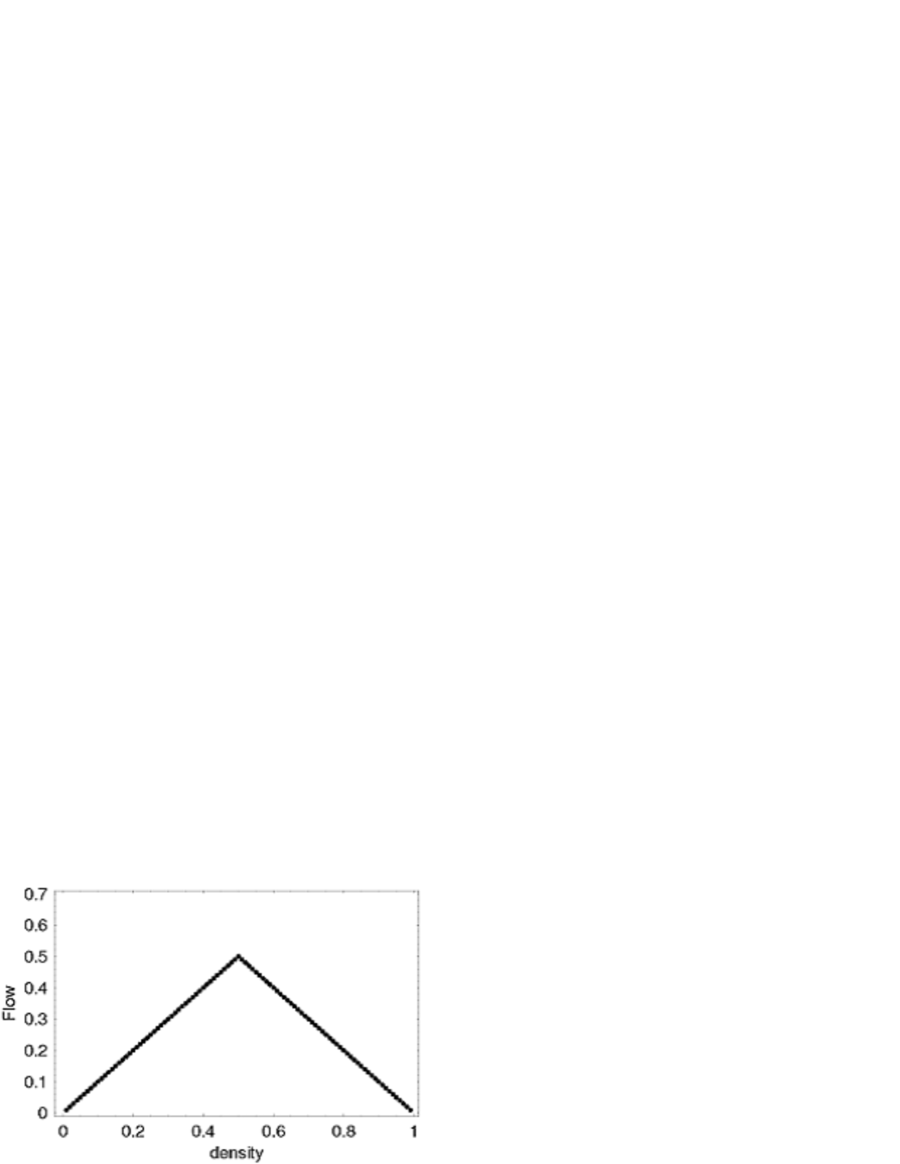
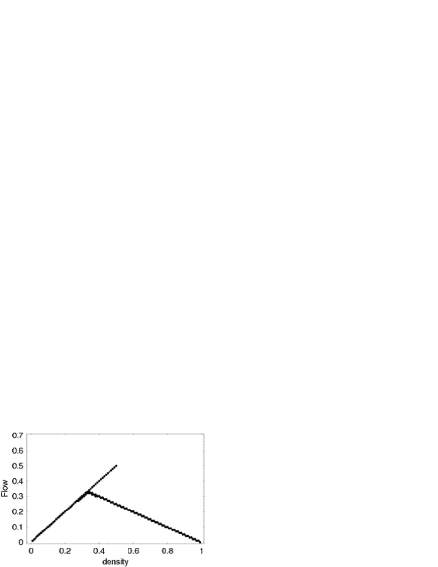
(a)$q=0.0$, $r=0.0$	(b)$q=0.5$, $r=0.0$	(c)$q=1.0$, $r=0.0$
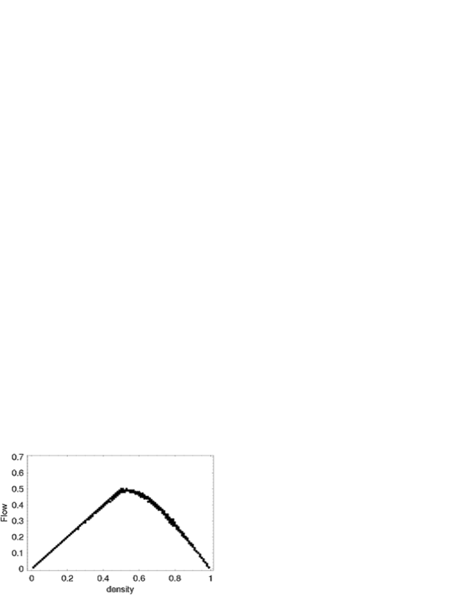
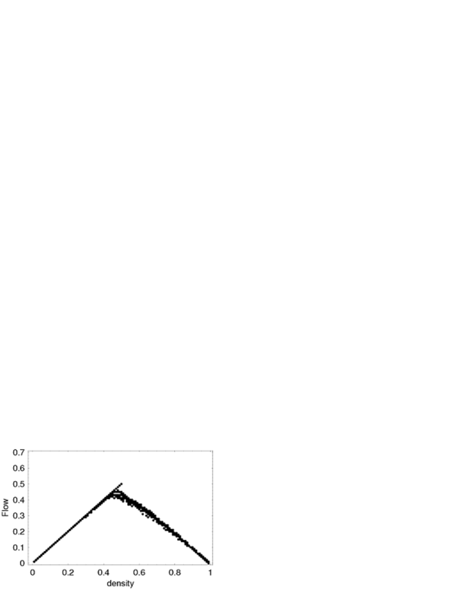
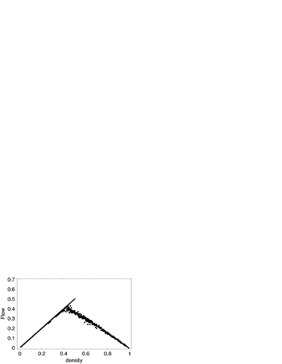
(d)$q=0.0$, $r=0.5$	(e)$q=0.5$, $r=0.5$	(f)$q=1.0$, $r=0.5$
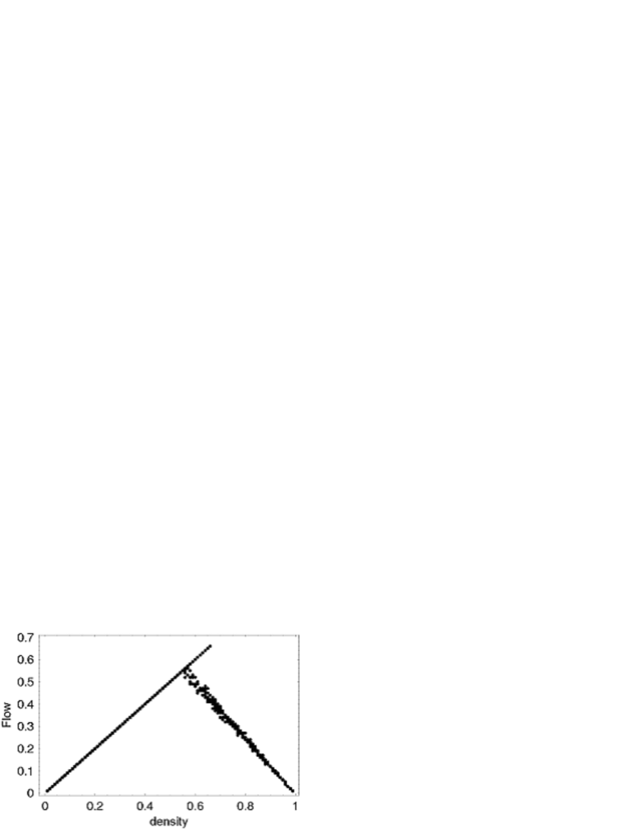
(g)$q=0.0$, $r=1.0$	(h)$q=0.5$, $r=1.0$	(i)$q=1.0$, $r=1.0$

Figure 3: Fundamental diagrams of S-NFS model with $p=1.0$, $L=100$ and $V_{\max}=1$. We repeat simulations for 10 initial conditions at each density. The flow is averaged over the range from $t=50$ to $t=100$. When $q\neq 0$ and for uniform initial distributions, metastable branches are clearly seen.

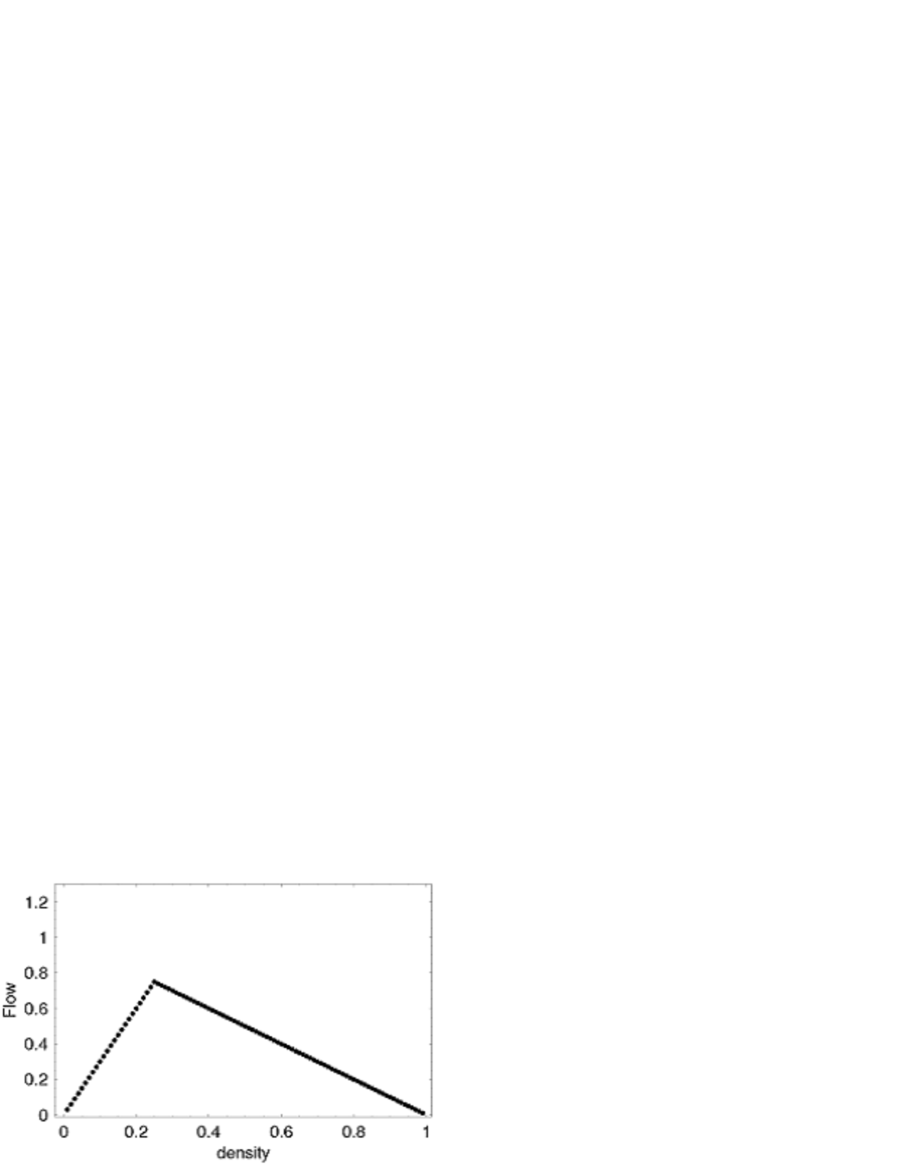
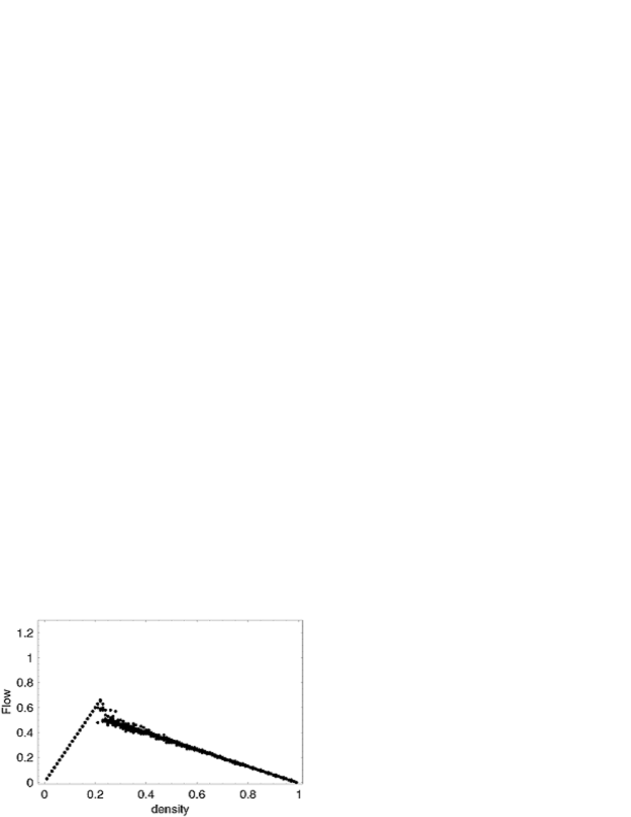
(a)$q=0.0$, $r=0.0$	(b)$q=0.5$, $r=0.0$	(c)$q=1.0$, $r=0.0$
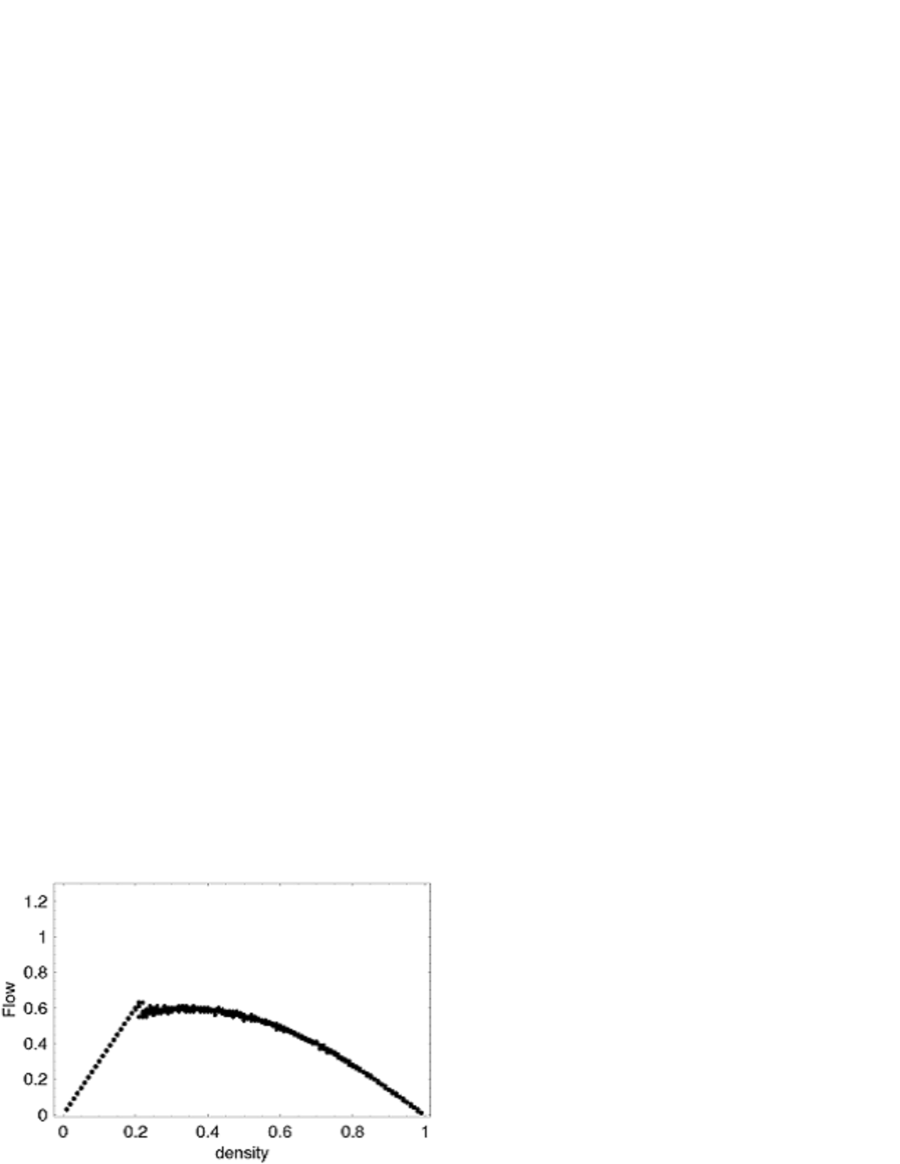
(d)$q=0.0$, $r=0.5$	(e)$q=0.5$, $r=0.5$	(f)$q=1.0$, $r=0.5$
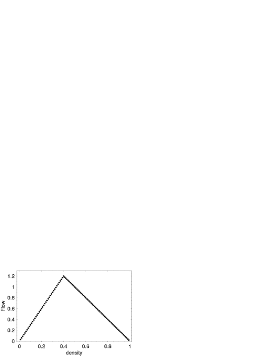
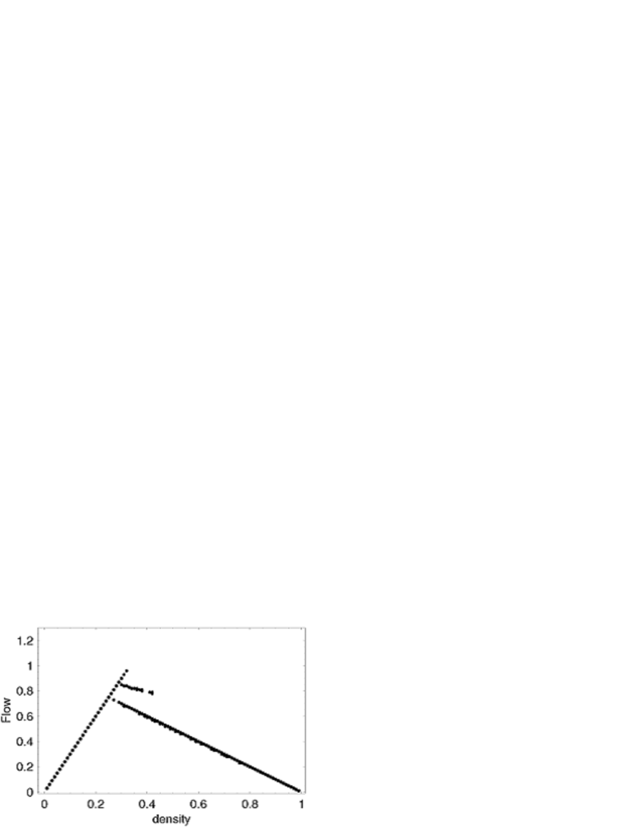
(g)$q=0.0$, $r=1.0$	(h)$q=0.5$, $r=1.0$	(i)$q=1.0$, $r=1.0$

Figure 4: Fundamental diagrams of S-NFS model with $p=1.0$, $L=100$ and $V_{\max}=3$. Contrary to the cases with $V_{\max}=1$, metastable states can remain even for random initial distributions.

The following two points are worthwhile to be mentioned;

(1)

Although free flow and jamming lines are both straight for $r=0$ or $r=1.0$, the shape of jamming lines are roundish for $r=0.5$ (see figures 3-(d) or 4-(d),(e),(f)) like ASEP with random braking effect ($p<1.0$). The origin of this behavior is as follows: Two successive cars can move simultaneously as long as $S=2$. However, once $S$ of a car moving rear changes to $1$, this car must stop. Hence random change of $S$ plays a similar role as random braking.

(2)

As is seen in figure 4-(h), metastable states “stably” exist even in the presence of stochastic effects, although in many other models metastable states soon vanish due to any perturbations. There are also some new branches around the critical density in our model. As seen in figure 1, these new branches may be related to the wide scattering area around the density $60$–$125$ ($\mbox{vehicles}/\mbox{km}$) in the observed data. Thus we believe we have successfully reproduce the metastable branches observed “stably” in the empirical data.

4 Phase diagram

In this section, we consider phase diagrams of S-NFS model with open boundary condition (OBC) when $V_{\max}=1$. Figure 5 shows our update rules for OBC:

1)

We put two cells at the sites $-2,-1$. At each site a car is injected with probability $\alpha$. The car’s velocity is set to $1$.

2)

We put cells at the sites $L,L+1$, and at each site a car is injected with probability $1-\beta$ (an outflow of a car from right end is obstructed by these cars). It’s velocity is set to $0$.

3)

Besides, we put cells at the sites $L+2,L+3$. At these two sites cars are always injected (this rule means that for cars at sites $-2,\ldots,L+1$, there exist at least two preceding cars at any time). It’s velocity is set to $0$.

4)

We apply updating rule of S-NFS to cars at sites $-2,\ldots,L+1$. However slow-to-start effect (7) apply only if $0\leq x_{i}^{t-1}$ and $x_{i+S}^{t-1}\leq L-1$.

5)

We remove all cars at $-2,-1$ and $L,\ldots,L+3$ at the end of each time step.

Figure 5: Updating rules for an open boundary condition of S-NFS model when $V_{\max}=1$. (a): Update rules (6)–(11) are applied to cars within this region. (b): The rule of slow-to-start (7) is effective only when $0\leq x_{i}^{t-1}$ and $x_{i+S}^{t-1}\leq L-1$.

These rules are devised in order to avoid unnatural traffic jam caused by boundary conditions. Here, the rule 3) is needed in order that for cars at sites $-2,\ldots,L+1$ there always exist at least two preceding cars. We need to apply S-NFS update rules to cars at sites $L,L+1$ because otherwise the velocity of the car at site $L-1$ is determined irrepective of the state at $L+1$ even when $S=2$.

With use of this boundary condition, we can calculate flow-$\alpha$-$\beta$ diagrams (see figure 7) form which phase diagrams are derived (see figures 12). The phase diagram of ASEP has been already known (see figure 6). In this diagram, the whole $\alpha$-$\beta$ region is divided into two phases in the case $p=1.0$: low-density (LD) phase which is “$\alpha$ controlled phase”; and high-density (HD) phase which is “$\beta$ controlled phase”. On the phase transition curve, the effect of $\alpha$ is balanced with that of $\beta$, and then these two phases coexist. The flow-$\alpha$-$\beta$ diagrams of S-NFS model are considerably different form the result of ASEP (see figure 7). The difference will be discussed in sec.5. We restrict ourselves to the case $V_{\max}=1$ and $p=1.0$ in the following.

(a)flow-$\alpha$-$\beta$ diagram

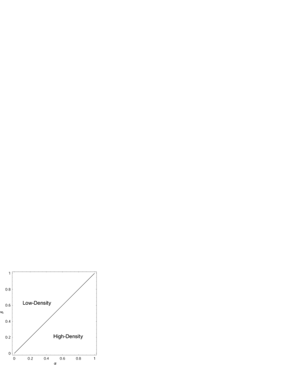
(b)$\alpha$-$\beta$ phase diagram

Figure 6: Definition of flow-$\alpha$-$\beta$ diagram of ASEP ($p=1.0,q=r=0.0$) and a corresponding $\alpha$-$\beta$ phase diagram. The line of the first-order phase transition is given by $\alpha=\beta$.

(a)$q=0.0$, $r=0.0$	(b)$q=0.5$, $r=0.0$	(c)$q=1.0$, $r=0.0$
(d)$q=0.0$, $r=0.5$	(e)$q=0.5$, $r=0.5$	(f)$q=1.0$, $r=0.5$
(g)$q=0.0$, $r=1.0$	(h)$q=0.5$, $r=1.0$	(i)$q=1.0$, $r=1.0$

Figure 7: Flow-$\alpha$-$\beta$ diagrams of S-NFS model with $p=1.0$ and $V_{\max}=1$. Note that flow suddenly rises near $\beta=1.0$ in (b), (c), (h), and (i) because cars never take the slow-to-start mode even when $q\neq 0$.

5 Phase transition curve

In this section, let us derive an analytic expression of the first-order phase transition curve of S-NFS model by combining approximate flow-density relations at boundaries and fundamental diagrams. We extend the method proposed in articles [11, 12]. The method consists of three steps: first, we relate the flow and density near the boundaries of the system in OBC; next, in fundamental diagrams of PBC, we calculate the gradient of free-flow line and jamming line; finally we can obtain phase diagrams for OBC from the above results.

5.1 Relation between flow and density near the boundaries

First, we calculate each flow $J_{l}$ and $J_{r}$ at left or right end of this system. Configurations in figure 8 contribute flow at each boundaries. Then with use of mean-field approach, the probability of the configration (a) is $c_{(-1)}[1-c_{(0)}]$. Similarly the probabilities of (b), (c), and (d) are $rc_{(-1)}c_{(0)}[1-c_{(1)}]$, $c_{(L-1)}[1-c_{(L)}]$, and $rc_{(L-1)}c_{(L)}[1-c_{(L+1)}]$ respectively. Here, $c_{(j)}$ denotes the probability of finding a car at the site $j$. Because $c_{(-1)}=\alpha$ and $c_{(L)}=c_{(L+1)}=1-\beta$, we get

$$\left\{\begin{array}[]{l}J_{l}=\alpha(1-c_{(0)})(1+rc_{(0)})\\ J_{r}=\beta[1+r(1-\beta)]c_{(L-1)}\end{array}\right.$$ (12)

where we assume $c_{(0)}=c_{(1)}$. Note, we ignored possibility that a car at the site $0$ can not move by slow-to-start effect in (b).

(a)

(b)

(c)

(d)

Figure 8: Configurations of cars contributing to flow at left or right ends. Other configurations do not generate flow at both ends.

5.2 Approximate expression of fundamental diagrams

Next we approximate free-flow line and jamming line of PBC by straight lines as

$$\left\{\begin{array}[]{ll}J_{f}=\rho=c_{(0)}&\mbox{(free-flow line)}\\ J_{j}=x(1-\rho)=x(1-c_{(L-1)})&\mbox{(jamming line)}\end{array}\right.,$$ (13)

where $J_{f}$ and $J_{j}$ denote the flow of free-flow and jamming phases, and $x$ is a magnitude of the gradient of jamming line. Here, we need to get the relations between $x$ and $q$ or $r$. The parameter $x$ is related to the velocity of backward moving traffic clusters which we will calculate with use of mean-field approach.

Figure 9 shows the possible configurations at the right end of clusters. The symbols $u_{g}(t)\;$ $g\in\{0,\;1,\;2\}$ mean the probability of each configurations at time $t$. The subscript $g$ denotes the gradient of each configurations. For example, let us consider the probability that the configuration figure 9 (c) becomes (b) in the next time step, $u_{2}(t)\rightarrow u_{1}(t+1)$ (see figure 10).

(a) $u_{0}(t)$

(b) $u_{1}(t)$

(c) $u_{2}(t)$

Figure 9: The connection between parameter $u_{g}(t)$ and configurations of cars.

Figure 10: The case that $u_{2}(t)$ becomes $u_{1}(t+1)$.

In order that (b) occurs, the slow-to-start effect is not active for the car A (the probability $1-q$). The car B does not move when (i) the driver’s perspective is not active (the probability $1-r$) or (ii) although the driver’s perspective is active, the car B still halts due to slow-to-start effect (the probability $qr$). Thus we get the term $u_{2}(t)(1-q)(1-r+qr)$ which expresses the probability that $u_{2}(t)$ becomes $u_{1}(t+1)$. Considering other possibilities in the same way, we get the following recursion relations

$$u_{0}(t+1) = u_{1}(t)q(1-r)+u_{2}(t)q$$ (14)

$$u_{1}(t+1) = u_{0}(t)(1-r)+u_{1}(t)(1-r+qr)(1-q+qr)+u_{2}(t)(1-q)(1-r+qr)$$ (15)

$$u_{2}(t+1) = u_{0}(t)r+u_{1}(t)r(1-q)(1-q+qr)+u_{2}(t)r(1-q)^{2}.$$ (16)

We solve the equations (14), (15), and (16) for the steady state $u_{g}(t+1)=u_{g}(t)=u_{g}$, and we get

$$u_{0} = \frac{q[1-r+(1-q)r^{2}]}{1-2q^{2}r^{2}+q(1-r+r^{2})}$$ (17)

$$u_{1} = \frac{1-(1-q+q^{2})r}{1-2q^{2}r^{2}+q(1-r+r^{2})}$$ (18)

$$u_{2} = \frac{[1-q+q^{2}(1-r)]r}{1-2q^{2}r^{2}+q(1-r+r^{2})}.$$ (19)

Thus, we take the expectation $x=0u_{0}+1u_{1}+2u_{2}$, and obtain the answer:

$$x=x(q,r)=\frac{1+r-qr+q^{2}r-2q^{2}r^{2}}{1+q-qr+qr^{2}-2q^{2}r^{2}}.$$ (20)

The relations between $x$ and $q$ or $r$ obtained from numerical simulations are plotted and compared with eq.(20) in figure 11. The theoretical curve (20) gives good estimation of numerical results.

(a)$x$-$q$ diagram ($r=0.0$)

(b)$x$-$r$ diagram ($q=0.0$)

Figure 11: The relation between the gradient of jamming line $x$ and probabilities $q$ or $r$. The solid line denotes the approximate analytic result, and points denote results of numerical simulations. There seem some discrepancies in (b). The reason is that we assume the shape of jamming line in the fundamental diagram to be straight although it is actually roundish.

5.3 Derivation of phase transition curve

Finally, we derive phase transition curve for OBC from above results. From (12) and (13), we obtain the following equations

$$J_{f}=J_{l} \quad\Longrightarrow\quad c_{(0)}=\alpha[1-c_{(0)}][1+rc_{(0)}]$$ (21)

$$J_{j}=J_{r} \quad\Longrightarrow\quad x[1-c_{(L-1)}]=\beta[1+r(1-\beta)]c_{(L-1)},$$ (22)

which lead to

$$\displaystyle c_{(0)}=\frac{\alpha(r-1)-1+\sqrt{\alpha^{2}(1+2r+r^{2})+2\alpha(1-r)+1}}{2r\alpha}$$ (23)

$$\displaystyle c_{(L-1)}=\frac{x}{\beta[1+r(1-\beta)]+x}.$$ (24)

Using (13) and the equation $J_{f}=J_{j}$ which is the characteristic of two phase coexistence, we can get $c_{(0)}=x[1-c_{(L-1)}]$. Substituting (24) into this equation, we can express $\beta$ by $q$, $r$, $x$, and $\alpha$:

$$\beta=\frac{1+r}{2r}+\frac{\sqrt{[c_{(0)}-x]^{2}(1+r)^{2}+4rx[c_{(0)}-x]c_{(0)}}}{2r[c_{(0)}-x]}$$ (25)

where $c_{(0)}$ is written by $\alpha$ and $r$ as equation (23). This is the approximated curve of the phase boundary.

It should be noted that (23) and (25) are a singular when $r=0.0$. Expression (25) becomes

$$\beta = \frac{x\alpha}{x(1+\alpha)-\alpha}$$ (26)

in this singular case. Figure 12 gives a comparison between the approximate phase transition curve (25) and contour curves of flow-$\alpha$-$\beta$ diagram obtained from numerical simulations. The phase transition curves are very close to those obtained from numerical simulations. However we note that the shape of jamming line in the fundamental diagram is assumed to be straight as (13). Therefore we see the approximate result is not good in the high flow region (where $\alpha$ and $\beta$ are close to $1$) for figure 12-(d) because in this case the shape of jamming line is apparently roundish (see figure 3-(d)).

The phase diagram consists of LD and HD phases, but maximal-current (MC) phase does not appear. Driver’s anticipation effect make the area of HD phase smaller whereas the slow-to-start effect gives the opposite tendency. Phase transition curve which is straight for ASEP is bent downward by driver’s anticipation effect. However, if $q\neq 0$, the slow-to-start effect becomes dominant as flow increases.

The article [12] also discusses a phase diagram of a model which includes only slow-to-start effect. The structure of phase diagram is similar to those of figure 12-(c). S-NFS model shows more variety of phase diagrams.

According to [12], for large $\beta$ there appears the enhancement of the flow which looks like MC phase. The enhancement is due to the finite system size effect and vanishes with increasing system size. Figure 13 demonstrates the effects of system sizes on our results. The shape of flow does not change with increasing the system size. Since there does not appear a plateau at $\alpha=0.75$, we judge that MC phase does not exist when $p=1.0$ for S-NFS model.

(a)$q=0.0$, $r=0.0$	(b)$q=0.5$, $r=0.0$	(c)$q=1.0$, $r=0.0$
(d)$q=0.0$, $r=0.5$	(e)$q=0.5$, $r=0.5$	(f)$q=1.0$, $r=0.5$
(g)$q=0.0$, $r=1.0$	(h)$q=0.5$, $r=1.0$	(i)$q=1.0$, $r=1.0$

Figure 12: Approximate phase transition curves that are calculated by (25), and contour curves of flow-$\alpha$-$\beta$ diagram (Fig. 7). The theoretical curves are in good agreement with numerical results.

Figure 13: Flow is plotted against $\beta$ at $\alpha=0.25$ and $\alpha=0.75$ when $p=q=r=1.0$. The symbols $+$ ($\bullet$) represent data for $L=600$ ($L=3000$). Solid lines denote the approximate results (13) with (23), (24) and (25).

6 Summary and conclusions

In this paper, we have considered a stochastic extension of a traffic cellular automaton model recently proposed by one of the authors [7]. This model (which we call S-NFS model) contains three parameters which control random braking, slow-to-start, and driver’s perspective effects. With special choice of these parameters, S-NFS model is reduced to previously known traffic CA models such as NS model, QS model, SlS model etc.. Hence S-NFS model can be considered as an unified model of these previously known models. Next, we investigated fundamental diagrams of S-NFS model. The shape of fundamental diagram of S-NFS model is similar to that with use of empirical data. Especially the metastable branches, which are indispensable to reproduce empirical fundamental diagrams, clearly seen even when stochastic effects are present. This robustness of metastable branches in this model is advantageous because empirical data shows metastability even though stochastic effects always exist in real traffic. Thus we can expect that S-NFS model captures essential feature of empirical traffic flow and is very useful for investigating various traffic phenomena such as jamming phase transition as well as for application in traffic engineering. Finally, we investigated phase diagrams of S-NFS model with $V_{\max}=1$ and $p=1.0$. The analytic expression of phase transition curve is obtained from the approximate relations between flow and density near the boundary, together with approximate gradient of jamming lines in fundamental diagrams. The analytic phase transition curve successfully explains those of numerical simulations. Recently we have found that, in the case $p<1.0$ MC phase appears in the S-NFS model. The analysis on the cases $V_{\max}>1$ or $p<1.0$ will be reported elsewhere [20].

References

References

- [1] Chowdhury D, Santen L, and Schadschneider A 2000 Phys. Rep. 329 199
- [2] Nagel K and Schreckenberg M 1992 J. Phys. I France 2 2221
- [3] Takayasu M and Takayasu H 1993 Fractals 1 860
- [4] Barlovic R, Santen L, Schadschneider A, and Schreckenberg M 1998 Eur Phys. J. B 5 793
- [5] Fukui M and Ishimashi Y 1996 J. Phys. Soc. Japan 65 1868
- [6] Nishinari K and Takahashi D 2000 J. Phys. A: Math. Gen. 33 7709
- [7] Nishinari K, Fukui M, and Schadschneider A 2004 J. Phys. A: Math. Gen. 37 3101
- [8] Kanai M, Nishinari K, and Tokihiro T 2005 Phys. Rev. E 72 035102
- [9] Schadschneider A and Schreckenberg M 1998 J. Phys. A: Math. Gen. 31 L225
- [10] Rajewsky N, Santen L, Schadschneider A, and Schreckenberg M 1998 J. Stat. Phys. 92 151
- [11] Kolomeisky A B, Schütz G M, Kolomeisky E B, and Straley J P 1998 J. Phys. A: Math. Gen. 31 6911
- [12] Appert C and Santen L 2001 Phys. Rev. Lett. 86 2498
- [13] Ishibashi Y and Fukui M 2002 J. Phys. Soc. Jpn 71 2335
- [14] Sugiyama Y and Nakayama A 2003: in Emmerich H, Nestler B, and Schreckenberg M Interface and Transport Dynamics (Berlin, Heidelberg, New York: Springer-Verlag) 406
- [15] Ishibashi Y and Fukui M 1996 J. Phys. Soc. Jpn 65 2793
- [16] Jiang R, Wu Q S, and Wang B H 2002 Phys. Rev. E 66 036104; Huang D W and Huang W N 2003 67 068101; Jiang R, Wu Q S, and Wang B H 2003 67 068102
- [17] Huang D W 2005 Phys. Rev. E 72 016102
- [18] Wolfram S 1986 Theory and Applications of Cellular Automata (Singapore: World Scientific)
- [19] Kerner B S and Klenov S L 2002 J. Phys. A: Math. Gen. 35 L31
- [20] Sakai S, Nishinari K, and Iida S, in preparation