Comments on the entropy of seismic electric signals under time reversal

Abstract

We present recent data of electric signals detected at the Earth’s surface, which confirm the earlier finding [Phys. Rev. E 73, 031114 (2006)] that the value of the entropy in natural time as well as its value under time reversal are smaller than that of the entropy of a “uniform” distribution. Furthermore, we show that the scale dependence of the fluctuations of the natural time itself under time reversal provides a useful tool for the discrimination of seismic electric signals (critical dynamics) from noises emitted from manmade sources as well as for the determination of the scaling exponent.

In a time series comprising $N$ events, the natural time $\chi_{k}=k/N$ serves as an indexVarotsos et al. (2001, 2002) for the occurrence of the $k$-th event. In natural time analysis, the time evolution of the pair of the two quantities ($\chi_{k},Q_{k}$) is considered, where $Q_{k}$ denotes in general a quantity proportional to the energy released during the $k$-th event. In the case of dichotomous electric signals (SES) activities (i.e., low frequency $\leq 1$Hz electric signals that precede earthquakes, e.g., see Refs.Varotsos and Alexopoulos (1986); Varotsos et al. (1986); Varotsos (2005); Varotsos et al. (2003a)) $Q_{k}$ stands for the duration of the $k$-th pulse. The entropy $S$ in natural time is definedVarotsos et al. (2003b) as

$$S\equiv\langle\chi\ln\chi\rangle-\langle\chi\rangle\ln\langle\chi\rangle$$ (1)

where $\langle f(\chi)\rangle=\sum_{k=1}^{N}p_{k}f(\chi_{k})$ and $p_{k}=Q_{k}/\sum_{n=1}^{N}Q_{n}$. The value of the entropy upon considering the time reversal ${\cal T}$, i.e., ${\cal T}p_{k}=p_{N-k+1}$, is labelled by $S_{-}$.

SES activities (critical dynamics) exhibit infinitely ranged long range temporal correlationsVarotsos et al. (2003c, 2006a, 2006b) which are destroyedVarotsos et al. (2006b) after shuffling the durations $Q_{k}$ randomly. An interesting property emerged from the data analysis of several SES activities refers to the factVarotsos et al. (2006a) that both $S$ and $S_{-}$ values are smaller than the value of $S_{u}(=1/2\ln 2-1/4\approx 0.0966$) of a “uniform” distribution (defined in Refs. Varotsos et al. (2001); Varotsos et al. (2003b); Varotsos et al. (2004); Varotsos et al. (2005a), e.g. when all $p_{k}$ are equal), i.e.,

$$S,S_{-}<S_{u}$$ (2)

This finding, which does not holdVarotsos et al. (2005b) for “artificial” noises (AN) (i.e., electric signals emitted from manmade sources), has been also supported by numerical simulations, e.g., in fractional Brownian motion (fBm) time seriesVarotsos et al. (2006a) that have an exponent $\alpha_{DFA}$ resulted from the Detrended Fluctuation Analysis (DFA)Peng et al. (1994); Buldyrev et al. (1995) close to unity. We clarify that fBm (with a self-similarity index $H\approx 1$) has been foundWeron et al. (2005) as an appropriate type of modelling process for the SES activities. Thus, it seemsVarotsos et al. (2006a) that the validity of the relation (2) stems from infinitely ranged long range correlations. The scope of this paper is twofold: First, to provide the most recent experimental data that strengthen the validity of the relation (2), and second to point out the usefulness of the study of the fluctuations of the natural time itself under time reversal.

Figure 1 depicts an electric signal, consisting of a number of pulses, that has been recorded on November 14, 2006 at a station labelledEPA (a) PIR lying in western Greece (close to Pirgos city). This signal has been clearly collected at eleven measuring electric dipoles with electrodes installed at sites that are depicted in a map given in Ref.EPA (a). The signal is presented (continuous line in red) in Fig. 1(a) in normalized units, i.e., by subtracting the mean value and dividing by the standard deviation. (As for the actual amplitude -in $mV/km$- of this SES activityEPA (b), it is comparable to the one observed at the same station before the magnitude $M\approx 7.0$ earthquake that occurred on Jan 8, 2006, see Ref.Varotsos (2006).) For the reader’s convenience the corresponding dichotomous representation is also drawn in Fig. 1(a) with a dotted (blue) line, while in Fig. 1(c) we show (in red crosses) how the signal is read in natural time. The computation of $S$ and $S_{-}$ leads to the following values: $S=0.070\pm 0.012$, $S_{-}=0.051\pm 0.010$. As for the varianceVarotsos et al. (2001, 2002); Varotsos et al. (2003c, b) $\kappa_{1}\equiv\langle\chi^{2}\rangle-\langle\chi\rangle^{2}$, the resulting value is $\kappa_{1}=0.062\pm 0.010$. These values more or less obey the conditions $\kappa_{1}\approx 0.070$ and $S,S_{-}<S_{u}$ that have been found to hold for other SES activitiesVarotsos et al. (2006a).

A closer inspection of Fig. 1(a) also reveals the following experimental fact: An additional electric signal has been also detected (in the gray shaded area of Fig. 1(a)), which consists of pulses with markedly smaller amplitude than those of the SES activity discussed in the previous paragraph. This is reproduced (continuous line in red) in Fig. 1(b) in an expanded time scale and for the sake of the reader’s convenience its dichotomous representation is also marked by the dotted (blue) line, which leads to the natural time representation shown (dotted blue) in Fig. 1(c). The computation of $S$ and $S_{-}$ gives $S=0.077\pm 0.004$, $S_{-}=0.082\pm 0.004$, while $\kappa_{1}$ is found to be $\kappa_{1}=0.076\pm 0.005$. Hence, these values also obey the aforementioned conditions ($\kappa_{1}\approx 0.070$ and $S,S_{-}<S_{u}$) for its classification as an SES activity.

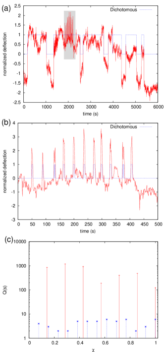
Figure 1: (color online) (a) The electric signal recorded on November 14, 2006 at PIR station (sampling rate $f_{exp}=1$Hz). The signal is presented here in normalized units (see the text). The corresponding dichotomous representation is shown with the dotted (blue) line. The gray shaded area shows an additional signal (consisting of pulses of smaller duration) superimposed on the previously mentioned signal. (b) The signal belonging to the gray shaded area in (a) is given here in an expanded time scale, while its dichotomous representation is marked by the dotted (blue) line. (c) How the signals in (a) and (b) are read in natural time: the continuous (red crosses) and dotted (blue asterisks) bars correspond to the durations of the dichotomous representations marked in (a) and (b), respectively.

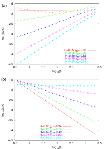
Figure 2: (color online) The log-log plot of the fluctuations $\Delta\chi_{l}$ of the natural time under time reversal versus the scale $l$ for fBm (a) and fGn (b). Time series of length $2\times 10^{4}$ have been used.

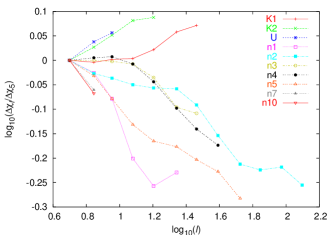
Figure 3: (color online) The log-log plot of $\Delta\chi_{l}$ versus the scale $l$ for three SES activities (K1, K2 and U) and seven AN (n1-n5, n7 and n10) treated in Ref.Varotsos et al. (2005b) (cf., these signals have enough number of pulses in order to apply the present analysis). The values of $\Delta\chi_{l}$ are divided by the corresponding values $\Delta\chi_{5}$ at the scale $l=5$.

We now proceed to the second goal of this paper. The way through which the entropy in natural time captures the influence of the effect of a small linear trend, has been studied in Ref.Varotsos et al. (2006a). Namely, the “uniform” distribution, $p(\chi)=1$, where $p(\chi)$ is a continuous probability density function (PDF) corresponding to the point probabilities $p_{k}$ used so far, has been perturbed by a linear trend $\epsilon$ in order to obtain the parametric family of PDFs: $p(\chi;\epsilon)=1+\epsilon(\chi-1/2)$. Such a family of PDFs shares the interesting property ${\cal T}p(\chi;\epsilon)=p(\chi;-\epsilon)$, i.e, the action of time reversal is obtained by simply changing the sign of $\epsilon$. It has been shownVarotsos et al. (2006a) that the entropy $S(\epsilon)\equiv S[p(\chi;\epsilon)]$, as well as that of the entropy under time reversal $S_{-}(\epsilon)\equiv S[{\cal T}p(\chi;\epsilon)]$, $S_{-}(\epsilon)=S(-\epsilon)$, depend non-linearly on the trend parameter $\epsilon$:

$$S(\epsilon)=-\frac{1}{4}+\frac{\epsilon}{72}-\left(\frac{1}{2}+\frac{\epsilon}{12}\right)\ln\left(\frac{1}{2}+\frac{\epsilon}{12}\right).$$ (3)

However, it would be extremely useful to obtain a linear measure of $\epsilon$ in natural time. Actually, this is simply the average of the natural time itself:

$$\langle\chi\rangle=\int_{0}^{1}\chi p(\chi;\epsilon)d\chi=\frac{1}{2}+\frac{\epsilon}{12}.$$ (4)

If we consider the fluctuations of this simple measure upon time-reversal, we can obtain information on the long-range dependence of $Q_{k}$. Actually, we shall show that a measure of the long-range dependence emerges in natural time if we study the dependence of its variance under time-reversal $\Delta\chi^{2}\equiv\text{E}[(\chi-{\cal T}\chi)^{2}]$ on the window length $l$ that is used for the calculation. Since ${\cal T}p_{k}=p_{l-k+1}$, we have

$$\Delta\chi^{2}\equiv\text{E}[(\chi-{\cal T}\chi)^{2}]=\text{E}\left\{\left[\sum_{k=1}^{l}\frac{k}{l}\left(p_{k}-p_{l-k+1}\right)\right]^{2}\right\},$$ (5)

where the symbol $\text{E}[\ldots]$ denotes the expectation value obtained when a window of length $l$ is sliding through the time series $Q_{k}$. By expanding the square in the last part of Eq.(5), we obtain

$$\Delta\chi^{2}=\sum_{k=1}^{l}\left(\frac{k}{l}\right)^{2}\text{E}[(p_{k}-p_{l-k+1})^{2}]+\sum_{k\neq m}\frac{km}{l^{2}}\text{E}[(p_{k}-p_{l-k+1})(p_{m}-p_{l-m+1})].$$ (6)

The basic relation that interrelates $p_{k}$ isVarotsos et al. (2004)

$$\sum_{k=1}^{l}p_{k}=1$$ (7)

or equivalently $p_{k}=1-\sum_{m\neq k}p_{m}$. By subtracting from the last expression, its value for $k=l-k+1$, we obtain $p_{k}-p_{l-k+1}=-\sum_{m\neq k}(p_{m}-p_{l-m+1})$, and thus

$$(p_{k}-p_{l-k+1})^{2}=-\sum_{m\neq k}(p_{k}-p_{l-k+1})(p_{m}-p_{l-m+1}).$$ (8)

By substituting Eq.(8) into Eq.(6), we obtain

$$\Delta\chi^{2}=-\sum_{k=1}^{l}\left(\frac{k}{l}\right)^{2}\sum_{m\neq k}\text{E}[(p_{k}-p_{l-k+1})(p_{m}-p_{l-m+1})]+\sum_{k\neq m}\frac{km}{l^{2}}\text{E}[(p_{k}-p_{l-k+1})(p_{m}-p_{l-m+1})]$$ (9)

which simplifies to

$$\Delta\chi^{2}=-\sum_{k,m}\frac{(k-m)^{2}}{l^{2}}\text{E}[(p_{k}-p_{l-k+1})(p_{m}-p_{l-m+1})]$$ (10)

The negative sign appears because $(p_{k}-p_{l-k+1})$ and $(p_{m}-p_{l-m+1})$ are in general anti-correlated due to Eq.(8). Equation (10) implies that $\Delta\chi^{2}$ measures the long-range correlations in $Q_{k}$: If we assume that $-\text{E}[(p_{k}-p_{l-k+1})(p_{m}-p_{l-m+1})]\propto(k-m)^{2\chi_{H}}/l^{2}$ (cf. $p_{k}$ scales as $1/l$, e.g. see Varotsos et al. (2004)), we have that $\Delta\chi^{2}\propto l^{4+2\chi_{H}}/l^{4}$ so that $\Delta\chi\propto l^{\chi_{H}}$ (where $\chi_{H}$ is a scaling exponent). In order to examine the validity of this result in the case when $Q_{k}$ are coming from a fractional Gaussian noise (fGn) or fBm, we employed the following procedure: First, we generated fBm (or fGn) time-series $X_{k}$ for a given value of $H$ using the Mandelbrot-Weierstrass functionMandelbrot and Wallis (1969); Szulga and Molz (2001); Frame et al. as described in Ref.Varotsos et al. (2006a). Second, since $Q_{k}$ should be positive, we normalized the resulting $X_{k}$ time-series to zero mean and unit standard deviation and then added to the normalized time-series $N_{k}$ a constant factor $c$ to ensure the positivity of $Q_{k}=N_{k}+c$ (for the purpose of the present study we used $c=10.0$). The resulting $Q_{k}$ time-series were then analyzed and the fluctuations of $\Delta\chi_{l}$ versus the scale $l$ are shown in Figure 2. We observe that for fBm the estimator $\chi_{H}\approx H$, whereas for fGn $\chi_{H}\approx H-1$. The physical meaning of the present analysis was further investigated by performing the same procedure in the time-series of the durations of the electric signals analyzed in Ref.Varotsos et al. (2005b). The relevant results are shown in Figure 3. Their inspection interestingly indicate that all seven AN correspond to descending $\Delta\chi_{l}$ curves versus the scale $l$, while the three SES to ascending curves. This fact is in essential agreement with the results obtained in Ref.Varotsos et al. (2003c), which showed that the SES activities have a stronger memory than AN. In other words, apart from being an estimator of the scaling behavior, the ascending or descending behavior of $\Delta\chi_{l}$ versus the scale $l$ seems to provide a useful new tool for the classification of a signal as SES activity or AN, respectively.

References

- Varotsos et al. (2001) P. A. Varotsos, N. V. Sarlis, and E. S. Skordas, Practica of Athens Academy 76, 294 (2001).
- Varotsos et al. (2002) P. A. Varotsos, N. V. Sarlis, and E. S. Skordas, Phys. Rev. E 66, 011902 (2002).
- Varotsos and Alexopoulos (1986) P. Varotsos and K. Alexopoulos, Thermodynamics of Point Defects and their Relation with Bulk Properties (North Holland, Amsterdam, 1986).
- Varotsos et al. (1986) P. Varotsos, K. Alexopoulos, K. Nomicos, and M. Lazaridou, Nature (London) 322, 120 (1986).
- Varotsos (2005) P. Varotsos, The Physics of Seismic Electric Signals (TERRAPUB, Tokyo, 2005).
- Varotsos et al. (2003a) P. Varotsos, N. Sarlis, and S. Skordas, Phys. Rev. Lett. 91, 148501 (2003a).
- Varotsos et al. (2003b) P. A. Varotsos, N. V. Sarlis, and E. S. Skordas, Phys. Rev. E 68, 031106 (2003b).
- Varotsos et al. (2003c) P. A. Varotsos, N. V. Sarlis, and E. S. Skordas, Phys. Rev. E 67, 021109 (2003c).
- Varotsos et al. (2006a) P. A. Varotsos, N. V. Sarlis, E. S. Skordas, H. K. Tanaka, and M. S. Lazaridou, Phys. Rev. E 73, 031114 (2006a).
- Varotsos et al. (2006b) P. A. Varotsos, N. V. Sarlis, E. S. Skordas, H. K. Tanaka, and M. S. Lazaridou, Phys. Rev. E 74, 021123 (2006b).
- Varotsos et al. (2004) P. A. Varotsos, N. V. Sarlis, E. S. Skordas, and M. S. Lazaridou, Phys. Rev. E 70, 011106 (2004).
- Varotsos et al. (2005a) P. A. Varotsos, N. V. Sarlis, E. S. Skordas, and M. S. Lazaridou, Phys. Rev. E 71, 011110 (2005a).
- Varotsos et al. (2005b) P. A. Varotsos, N. V. Sarlis, H. K. Tanaka, and E. S. Skordas, Phys. Rev. E 71, 032102 (2005b).
- Peng et al. (1994) C.-K. Peng, S. V. Buldyrev, S. Havlin, M. Simons, H. E. Stanley, and A. L. Goldberger, Phys. Rev. E 49, 1685 (1994).
- Buldyrev et al. (1995) S. V. Buldyrev, A. L. Goldberger, S. Havlin, R. N. Mantegna, M. E. Matsa, C.-K. Peng, M. Simons, and H. E. Stanley, Phys. Rev. E 51, 5084 (1995).
- Weron et al. (2005) A. Weron, K. Burnecki, S. Mercik, and K. Weron, Phys. Rev. E 71, 016113 (2005).
- EPA (a) eprint See EPAPS Document No. E-PLEEE8-74-190608 for additional information, originally from P.A. Varotsos, N.V. Sarlis, E.S. Skordas, H.K. Tanaka and M.S. Lazaridou, Phys. Rev. E 74, 021123 (2006). For more information on EPAPS, see http://www.aip.org/pubservs/ epaps.html.
- EPA (b) eprint The time of the impending earthquake can be determined by means of the procedure described in EPAPS Document No. E-PLEEE8-73-134603 for additional information, originally from P.A. Varotsos, N.V. Sarlis, E.S. Skordas, H.K. Tanaka and M.S. Lazaridou, Phys. Rev. E 73, 031114 (2006). For more information on EPAPS, see http://www.aip.org/pubservs/ epaps.html.
- Varotsos (2006) P. A. Varotsos, Proc. Japan Acad., Ser. B 82, 86 (2006).
- Mandelbrot and Wallis (1969) B. Mandelbrot and J. R. Wallis, Water Resources Research 5, 243 (1969).
- Szulga and Molz (2001) J. Szulga and F. Molz, J. Stat. Phys. 104, 1317 (2001).
- (22) M. Frame, B. Mandelbrot, and N. Neger, fractal Geometry, Yale University, available from http://classes.yale.edu/fractals/, see http://classes.yale.edu/Fractals/RandFrac/fBm/fBm4.html.