Rectification effects in coherent transport through single molecules

Abstract

A minimal model for coherent transport through a donor/acceptor molecular junction is presented. The two donor and acceptor sites are described by single levels energetically separated by an intramolecular tunnel barrier. In the limit of strong coupling to the electrodes a current rectification for different bias voltage polarities occurs. Contacts with recent experiments of molecular rectification are also given.

1 Introduction

In recent years, molecular electronics has gained considerable attention due to the viability to measure quantum transport observables through single molecules. In fact, various effects typical of the physics of mesoscopic electron systems ranging from Coulomb blockade effects with weak coupling between the molecule and the leads to coherent transport through strongly bonded molecules have been observed [1, 2]. However, it is desirable to obtain clear relationships between truly intrinsic molecular properties and measured effects. For example, vibron assisted tunneling [3] or current switching due to a controllably induced conformational change of the molecular shape [4, 5] have been observed. Another idea, firstly proposed theoretically by Aviram and Ratner [6], is to create molecules able to rectify electric currents, i.e. $I(U)\neq-I(-U)$. This can be either achieved by distinct asymmetric molecules (e.g. asymmetric tunneling barriers between the contacts and a central part of the molecule [7]) or by an intrinsic modification of the electronic properties of the molecules [8, 9].

2 System and Method

Having in mind the experiments by Elbing et al. [9], where a molecule consisting of two broken $\pi$-conjugated donor/acceptor subunits connected to gold electrodes via thiol groups showed a diode-like behavior, a minimal model for quantum transport through such a molecular system is presented. Though lacking ab initio accuracy, our model gives a basic insight to the mechanism of molecular rectification.
We describe the donor-acceptor molecule by two single levels separated by a tunneling junction. The on-site energies are $\epsilon_{11}^{0}$ and $\epsilon_{22}^{0}$ (in the case of the isolated molecule), respectively (see Fig. 1). These energies are measured relatively to the Fermi energies of the electrodes, which are both set arbitrarily to zero. The two parts of the molecule are coupled by a weakly conducting bridge, which can be formed by a $\sigma$-bond [6] or an almost broken biphenylic $\pi$-bond [9].

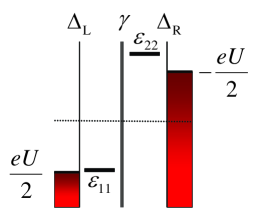
(a) $U<0$

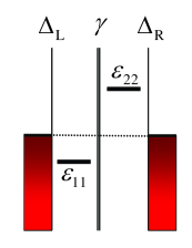
(b) $U=0$

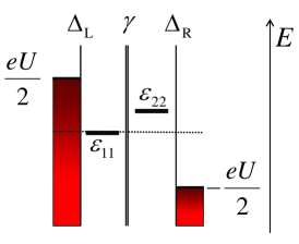
(c) $U>0$

Figure 1: Sketch of the energy levels at negative (a), zero (b) and positive (c) bias voltage. The dotted lines indicate the position of the Fermi energy. Since the molecular levels themselves are affected by the bias voltage, Eq. (1), the distance and positions of the levels are strongly sensitive to the bias polarity.

Under the external bias voltage $U$, which is applied symmetrically on the two contacts, the chemical potentials of left and right lead are moved: $\mu_{\mathrm{L}}=-\mu_{\mathrm{R}}=eU/2$. Furthermore, the energy levels of the molecular sites are shifted as

$$\epsilon_{11}\left(U\right)=\epsilon_{11}^{0}+\eta_{1}eU,\quad\epsilon_{22}\left(U\right)=\epsilon_{22}^{0}+\eta_{2}eU.$$ (1)

To implement the fact that the bottleneck tunneling barrier in the system would tend to pin these levels to the nearby electrode, we assume that one fourth of the applied voltage drops at the contacts between the molecule and the leads and one half of the bias voltage drops in the middle of the system between the two parts of the molecule at the intra-molecular barrier, i.e. $\eta_{1}=-\eta_{2}=0.25$, this assumption is then lifted at the end of this paper when discussing different strengths of coupling between electrodes and molecule.
The Hamiltonian describing the molecule is given by

$$H_{\mathrm{M}}=\sum_{\alpha,\beta=1,2}\epsilon_{\alpha\beta}\left(U\right)c_{\alpha}^{\dagger}c_{\beta}^{\phantom{\dagger}}+\textrm{H.c.},$$ (2)

whereas the diagonal elements $\epsilon_{\alpha\alpha}$ are defined by the on-site energies $\epsilon_{\alpha\alpha}\left(U\right)$ and the off diagonal elements $\epsilon_{12}$ and $\epsilon_{21}$ are given by the hopping parameter between the two levels, $-\gamma$, which is a measure for the inter-site coupling. In the two dimensional base of the localized orbital operators the Hamiltonian matrix simply writes:

$$\bf{H}_{\mathrm{M}}=\left(\begin{array}[]{cc}\epsilon_{11}\left(U\right)&-\gamma\\ -\gamma&\epsilon_{22}\left(U\right)\end{array}\right).$$ (3)

The total Hamiltonian contains two additional terms due to the electrodes and their coupling to the molecule: $H=H_{\mathrm{M}}+H_{\mathrm{M-leads}}+H_{\mathrm{leads}}.$ To calculate the spectral and transport properties of the molecule coupled to leads, we use the nonequilibrium Green functions technique for finite bias voltage without interaction. The retarded Green function matrix of the molecular region dressed by the electrode self-energies reads [10]

$$\left(\bf{G}^{\textrm{r}}\right)^{-1}=\left(\left(E+\textrm{i}0^{+}\right)\bf{1}-\bf{H}_{\mathrm{M}}-\bf{\Sigma}_{\mathrm{L}}-\bf{\Sigma}_{\mathrm{R}}\right),$$ (4)

where

$$\bf{\Sigma}_{\mathrm{L}}=\left(\begin{array}[]{cc}-\textrm{i}\Delta_{\mathrm{L}}&0\\ 0&0\end{array}\right),\quad\bf{\Sigma}_{\mathrm{R}}=\left(\begin{array}[]{cc}0&0\\ 0&-\textrm{i}\Delta_{\mathrm{R}}\end{array}\right)$$ (5)

are the self-energy matrices of left and right lead, which already lift the molecular resonances away from the real energy axis, surrogating the need of a small imaginary shift applied in the definition of the retarded Green function. For the self-energies we use the wide band approximation, which assumes a purely imaginary energy-independent self-energy. $\Delta_{\mathrm{L,R}}$ describe the hopping between the contacts and the two energy levels. Both $\Delta_{\mathrm{L}}$ and $\Delta_{\mathrm{R}}$ are assumed to be constant positive real numbers with no energy dependence (wide band approximation). This is a reasonable assumption when thinking of gold electrodes whose bands are more extended than the molecular active energetic window. The transmission probability is obtained from the Green function by the Fisher-Lee relation $T\left(E,U\right)=\left\{\bf{\Gamma}_{\mathrm{L}}\bf{G}^{\mathrm{r}}\bf{\Gamma}_{\mathrm{R}}\bf{G}^{\mathrm{r}\dagger}\right\}$ [11, 12] with the matrices $\bf{\Gamma}_{\mathrm{L}}=\textrm{i}\left(\bf{\Sigma}_{\mathrm{L}}^{\phantom{\dagger}}-\bf{\Sigma}_{\mathrm{L}}^{\dagger}\right)$ and $\bf{\Gamma}_{\mathrm{R}}=\textrm{i}\left(\bf{\Sigma}_{\mathrm{R}}^{\phantom{\dagger}}-\bf{\Sigma}_{\mathrm{R}}^{\dagger}\right)$ as the anti-Hermitian parts of the self-energy matrices of the contacts.
In the case of the two site-model studied here, it is easy to obtain an analytical expression for the transmission probability as a function of voltage and charge injection energy:

$$T\left(E,U\right) = 4\Delta_{\mathrm{L}}\Delta_{\mathrm{R}}\left|G_{12}^{\textrm{r}}\right|^{2}=4\Delta_{\mathrm{L}}\Delta_{\mathrm{R}}\gamma^{2}/\left(A+B\right)$$ (6)

$$A = \left[\left(E-\epsilon_{11}\left(U\right)\right)\left(E-\epsilon_{22}\left(U\right)\right)-\gamma^{2}-\Delta_{\mathrm{L}}\Delta_{\mathrm{R}}\right]^{2}$$

$$B = \left[\Delta_{\mathrm{L}}\left(E-\epsilon_{11}\left(U\right)\right)+\Delta_{\mathrm{R}}\left(E-\epsilon_{22}\left(U\right)\right)\right]^{2}.$$

Knowing the transmission probability, the current through the system can be obtained by the relation [12]:

$$I\left(U\right)=\frac{2e}{h}\int\mathrm{d}E\;\;T\left(E,U\right)\left(f_{\mathrm{L}}\left(E\right)-f_{\mathrm{R}}\left(E\right)\right).$$ (7)

Here, $f_{\mathrm{L},\mathrm{R}}\left(E\right)=f\left(E-\mu_{\mathrm{L},\mathrm{R}}\right)$ are the Fermi functions of left and right electrode depending on the bias voltage and the temperature, which in our calculations is set to $30$ K. To understand the evolution of the molecular levels under the influence of the applied bias voltage and the coupling to the leads, we analyze the density of states (DOS), especially the localized density of states (LDOS) projected on the two sites of the molecule:

$$\mathrm{LDOS}_{\mathrm{1}}\left(E,U\right)=-\frac{1}{2\pi}\textrm{Im}\,\textrm{Tr}_{1}G^{\textrm{r}}=-\frac{1}{2\pi}\textrm{Im}G^{\textrm{r}}_{11},$$

$$\mathrm{LDOS}_{\mathrm{2}}\left(E,U\right)=-\frac{1}{2\pi}\textrm{Im}\,\textrm{Tr}_{2}G^{\textrm{r}}=-\frac{1}{2\pi}\textrm{Im}G^{\textrm{r}}_{22}.$$ (8)

Additionally, we define $\Delta_{\mathrm{DOS}}=\mathrm{LDOS}_{\mathrm{1}}-\mathrm{LDOS}_{\mathrm{2}}$ and $\Pi_{\mathrm{DOS}}=\mathrm{LDOS}_{\mathrm{1}}\cdot\mathrm{LDOS}_{\mathrm{2}}$. Looking at $\Delta_{\mathrm{DOS}}$, one can find the localization of a molecular level: positive $\Delta_{\mathrm{DOS}}$ implies that the state is more localized on site $1$, negative $\Delta_{\mathrm{DOS}}$ points to a pronounced state on site $2$. $\Pi_{\mathrm{DOS}}$, on the contrary, enhances with the equipartition of molecular states on the two sites.

3 Results and Discussion

The case of two identical sites $\epsilon_{11}^{0}=\epsilon_{22}^{0}$, independently of their value, leads straightforwardly to a symmetric behavior of the current with respect to an inversion of the applied bias, i.e. $I\left(U\right)=-I\left(-U\right)$. First, we want to study the case of two levels with different energies coupled symmetrically to the leads ($\Delta_{\mathrm{L}}=\Delta_{\mathrm{R}}=\Delta_{0}$). In the upper panel of Fig. 2, the difference of the DOS projected on the two levels is shown as a function of the applied bias voltage and the energy: the two lines show the variation of the two molecular levels which are broadened by the coupling to the leads. The localization of the levels is indicated as follows: red resp. black color of the central part indicates that the level is situated on site 1, blue points to a level localized on site 2. For large negative bias voltages, the two levels are far apart. With increasing voltage, the two levels approach each other, but do not cross and move away from each other again. This repulsion is quantified by the inter-site coupling $2\gamma$. At this voltage, $\Delta_{\mathrm{DOS}}$ is zero whereas $\Pi_{\mathrm{DOS}}$ takes its maximum (lower panel). After the avoided crossing, a change in the localization of the energy levels takes place.

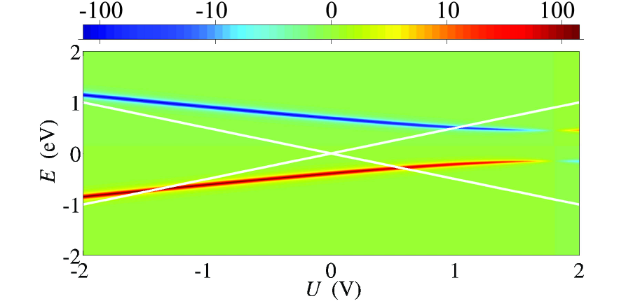
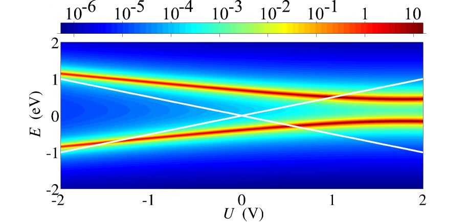
Figure 2: Difference (upper panel) and product (lower panel) of the localized density of states of site $1$ and site $2$ as a function of the bias voltage and the energy. The white lines indicate the bias window. In order to emphasize the molecular states, a logarithmic nonlinear scale has been applied. (Parameters: $\epsilon_{11}^{0}=-0.3$ eV, $\epsilon_{22}^{0}=0.6$ eV, $\Delta_{0}=0.02$ eV, $\gamma=0.3$ eV, $\eta_{1}=-\eta_{2}=0.25$).

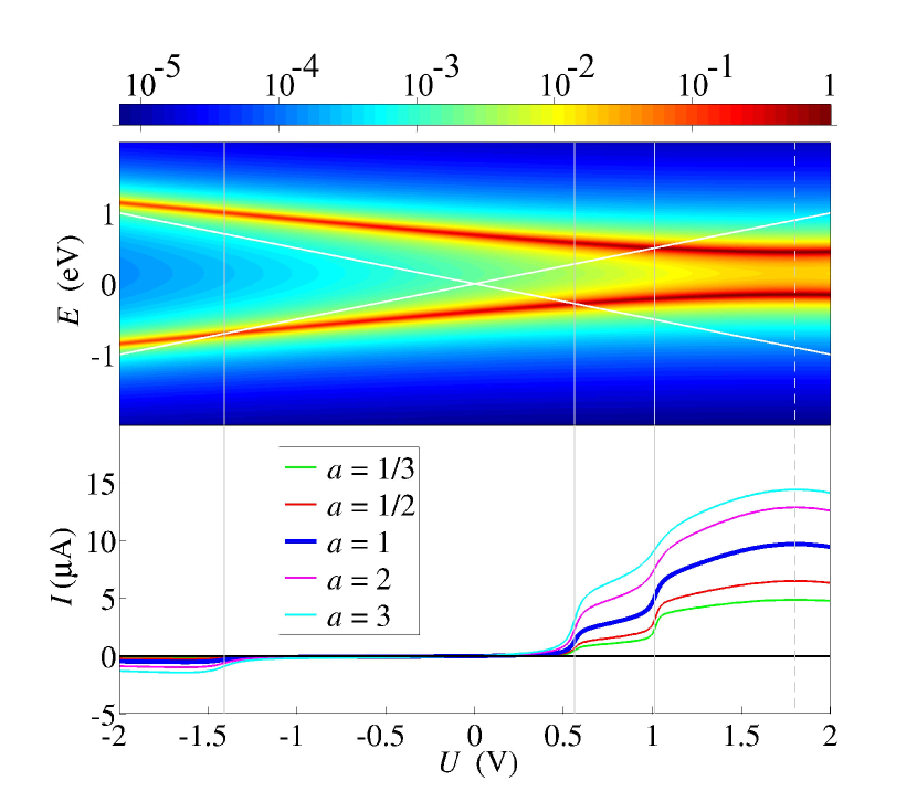
Figure 3: Transmission function $T\left(E,U\right)$ (upper panel, in a logarithmic scale) and current $I\left(U\right)$ (lower panel) for a two-site system. The white lines in the upper panel indicate the bias window. Different rectification degrees are obtained for different asymmetry parameters $a$, with $\Delta_{\mathrm{L}}=\Delta_{0}$ and $\Delta_{\mathrm{R}}=a\Delta_{0}$. (Parameters: $\epsilon_{11}^{0}=-0.3$ eV, $\epsilon_{22}^{0}=0.6$ eV, $\Delta_{0}=0.02$ eV, $\gamma=0.3$ eV, $\eta_{1}=-\eta_{2}=0.25$).

Fig. 3 shows the calculated transmission function and the current flowing through the system (thick blue line in the lower panel) calculated using Eq. (7). The bias window, indicated in the plot of the transmission function by the two white lines, is determined by the integration interval fixed because of the Fermi functions at low temperature. A step in the current-voltage curve appears, when a level enters the bias window, as it happens once at negative and once at positive bias voltages. If $\Delta_{0}$ is small compared to the level spacing, i.e. for relatively sharp molecular levels, the positions of the steps is given by the crossing of the eigenenergies (this can be determined analytically by a diagonalization of the Hamiltonian in Eq. (3)) and the lines defining the bias window. In our case, as depicted by the solid grey vertical lines in Fig. 3, this takes place at $U=-1.41$ V in negative bias direction and at $U=0.56$ V and $U=1.01$ V for positive bias. The height of the steps however depends crucially on the distance between the two levels: in the region of negative voltage, the two states are far apart and the height of the steps is therefore relatively small, whereas for positive bias voltage, the levels are much closer to each other, which results in a more resonant state and a much higher current. This explains the observed rectification in our model. The highest current is reached where the two levels are closest to each other. The peak in $I(U)$ appears at the bias voltage $\left(\epsilon_{22}^{0}-\epsilon_{11}^{0}\right)/e\left(\eta_{1}-\eta_{2}\right)$ (in our case $U=1.80$ V, depicted by the dashed grey line in Fig. 3) which can be obtained by a minimization of the energy gap between the two eigenenergies of the bare molecule [13]. For higher voltages, the distance between the levels grows again and the current decreases.
So far, we only considered symmetric coupling of the molecule to the leads. However, in experimental investigations of electronic transport through single molecules, the strength of the bonds between the molecule and the leads is mostly not well defined. Therefore, it is important to study the case of the molecule coupled asymmetrically to the electrodes, i.e. $\Delta_{\mathrm{L}}=a_{\mathrm{L}}\Delta_{0}$ and $\Delta_{\mathrm{R}}=a_{\mathrm{R}}\Delta_{0}$. The thin lines in Fig. 3 represent the values of the current for asymmetric coupling $a_{\mathrm{L}}=1$ and different values of $a_{\mathrm{R}}=a$, resulting in $\Delta_{\mathrm{L}}=\Delta_{0}$ and $\Delta_{\mathrm{R}}=a\Delta_{0}$. The other model parameters remain unchanged, especially $\eta_{1}=-\eta_{2}=0.25$. In this case, the general shape of the current curve does not change; the steps and the maximum in the current voltage curve do not change their positions, only the absolute values of the current are different due to the varying coupling to the leads. To understand the correct voltage drop along the molecule, one should use the Poisson equation with boundary conditions given by the applied bias voltage. This goes beyond the scope of this paper which concentrates on a simplified picture of the molecular electronic structure. Thus, in order to improve the plain effect of asymmetric coupling to the shape of the voltage drop along the system, we assume a larger voltage drop at the weaker contact. This changes as a consequence the values of the factors $\eta_{1,2}$ defined in Eq. (1) according to, e.g,: $\eta_{1}=\left(3a_{\mathrm{R}}-a_{\mathrm{L}}\right)/8$ and $\eta_{2}=\left(a_{\mathrm{R}}-3a_{\mathrm{L}}\right)/8,$ which for the case $a_{\mathrm{L}}=a_{\mathrm{R}}=1$ would restore the previously used values of $\eta_{1,2}$.

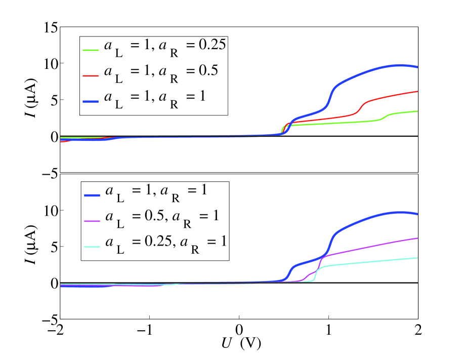
Figure 4: Current voltage characteristics for two cases of asymmetric coupling. In the upper panel, $a_{\mathrm{L}}=1$, the lower panel shows the case $a_{\mathrm{R}}=1$. (Parameters: $\epsilon_{11}^{0}=-0.3$ eV, $\epsilon_{22}^{0}=0.6$ eV, $\Delta_{0}=0.02$ eV, $\gamma=0.3$ eV, $\eta_{1}=-\eta_{2}=0.25$).

The results for this refined model are shown in Fig 4, the thick blue line again representing the symmetric case. Here, the position of the steps is shifted to different voltages. As it becomes evident from a comparison of Figs. 3 and 4, different shapes of the voltage drop imply a shift of the position where the current significantly changes, i.e. where the steps appear. Rectification effects due to the asymmetric coupling as shown in Fig. 3, have been already reported in the literature [14] but we here we want to stress that the precise value of the current jumps are not a mere electronic structure effect, but also depend on the profile of the electric field under the fixed applied bias voltage.

4 Conclusions and Outlook

In this paper, we have shown a minimal model for rectification effects in coherent transport through single molecules which was inspired by recently published experiments [9]. An extension to this model includes charging effects [15], taking into account on-site correlations on the two molecular sites, which becomes important in the case of a weak coupling between the molecule and the electrodes. These implementations though do not essentially change the nature of the effects observed in the picture discussed here, except for a natural splitting of conductance steps due to the lifting of the spin degeneracy induced by the correlation effects. Additionally, density functional theory can be used to calculate the positions of the energy levels of the molecule and their exact behavior under each bias voltage applied to the molecule, combined with a calculation of the correct voltage drop distribution at this voltage solving the Poisson equation. Together with nonequilibrium Green functions, this procedure allows to calculate the transmission $T\left(E,U\right)$ and the current $I\left(U\right)$, and not only the electronic structure under an applied voltage, in a truly ab initio way. Such study is currently under investigation [16].

5 Acknowledgements

We thank Bo Song and Dmitry A. Ryndyk for useful discussions. This work has been supported by the Volkswagen Foundation grant Nr. I/78-340.

References

- [1] A. Nitzan, M. A. Ratner, Electron transport in molecular wire junctions, Science 300 (5624) (2003) 1384.
- [2] G. Cuniberti, G. Fagas, K. Richter (Eds.), Introducing molecular electronics, Springer, Berlin, 2005.
- [3] M. Reed, W. Wang, T. Lee, Intrinsic electronic conduction mechanisms in self-assembled monolayers, [2].
- [4] F. Moresco, G. Meyer, K.-H. Rieder, H. Tang, A. Gourdon, C. Joachim, Conformational changes of single molecules induced by scanning tunneling microscopy manipulation: A route to molecular switching, Phys. Rev. Lett. 86 (4) (2001) 672.
- [5] X. Qiu, G. Nazin, W. Ho, Mechanisms of reversible conformational transitions in a single molecule, Phys. Rev. Lett. 93 (19) (2004) 196806.
- [6] A. Aviram, M. A. Ratner, Molecular rectifiers, Chem. Phy. Lett. 29 (2) (1974) 277.
- [7] P. Kornilovitch, A. Bratkovsky, R. S. Williams, Current rectification by molecules with asymmetric tunneling barriers, Phys. Rev. B 66 (16) (2002) 165436.
- [8] R. Metzger, Unimolecular electrical rectifiers, Chem. Rev. 103 (9) (2002) 3803.
- [9] M. Elbing, R. Ochs, M. Koentopp, M. Fischer, C. von Hänisch, F. Weigend, F. Evers, H. B. Weber, M. Mayor, A single-molecule diode, Proc. Natl. Acad. Sci. USA 102 (25) (2005) 8815.
- [10] G. Cuniberti, R. Gutiérrez, F. Grossmann, The role of contacts in molecular electronics, Advances in Solid State Physics 42 (2002) 133.
- [11] D. S. Fisher, P. A. Lee, Relation between conductivity and transmission matrix, Phys. Rev. B 23 (12) (1981) 6851.
- [12] S. Datta, Electronic Transport in Mesoscopic Systems, Cambridge University Press, Cambridge, 1999.
- [13] S. Lakshmi, S. K. Pati, Current-voltage characteristics in donor-acceptor systems: Implications of a spatially varying electric field, Phys. Rev. B 72 (19) (2005) 193410.
- [14] S. Datta, W. Tian, S. Hong, R. Reifenberger, J. I. Henderson, C. P. Kubiak, Current-voltage characteristics of self-assembled monolayers by scanning tunneling microscopy, Phys. Rev. Lett. 79 (13) (1997) 2530.
- [15] B. Song, D. A. Ryndyk, G. Cuniberti, Molecular junctions in the Coulomb blockade regime: rectification and nesting, preprint (2006), cond-mat/0611190.
- [16] F. Pump, A. Pecchia, A. Di Carlo, G. Cuniberti, in preparation.