Numerical ansatz for solving integro-differential equations with increasingly smooth memory kernels: spin-boson model and beyond

Abstract

We present an efficient and stable numerical ansatz for solving a class of integro-differential equations. We define the class as integro-differential equations with increasingly smooth memory kernels. The resulting algorithm reduces the computational cost from the usual $T^{2}$ to $TC\left(T\right)$, where $T$ is the total simulation time and $C\left(T\right)$ is some function. For instance, $C\left(T\right)$ is equal to $\ln T$ for polynomially decaying memory kernels. Due to the common occurrence of increasingly smooth memory kernels in physical, chemical, and biological systems, the algorithm can be applied in quite a wide variety of situations. We demonstrate the performance of the algorithm by examining two cases. First, we compare the algorithm to a typical numerical procedure for a simple integro-differential equation. Second, we solve the NIBA equations for the spin-boson model in real time.

1 Introduction

A major problem in the study of quantum systems is the influence of the environment on its dynamics. A variety of techniques, such as the influence functional [1], nonequilibrium perturbation theory [2, 3], and the weak-coupling approximation [4], have been developed to address this issue. The general approach is to derive equations of motion which only involve the degrees of freedom of the system. When working with systems weakly coupled to a rapidly relaxing environment, one can make the Markov approximation, which results in a local in time, first-order differential equation. This Markovian master equation is relatively easy to solve either analytically or numerically. As soon as the restrictions of weak coupling or fast environmental relaxation are removed, however, integro-differential equations appear, which reflects the fact that the environment retains a memory of the system at past times.

In particular, a number of interesting physical systems have integro-differential equations of motion with polynomially decaying memory kernels. For instance, the spin-boson model [5] and Josephson Junctions with quasi-particle dissipation or resistive shunts [6] have $1/t^{2}$ asymptotic kernels when going through a dissipatively driven phase transition. The occurrence of polynomially decaying kernels is common in physics and chemistry because many open systems are connected to an ohmic environment. Polynomially decaying kernels appear in biological applications as well. [7] Due to the frequent appearance of this type of kernel and also others which satisfy a requirement we call increasingly smooth below, it would be beneficial to have efficient numerical methods to handle the corresponding integro-differential equations. Such a method will be useful in applications in many disciplines. In addition, the method will enable the simulation of memory-dependent dissipation when used in conjunction with other computational methodologies, such as matrix product state algorithms for open systems. [8, 9, 10, 11]

In this paper, we give an efficient and stable numerical ansatz for solving integro-differential equations with increasingly smooth memory kernels. Using typical techniques, one incurs a computational cost of $AT^{2}\propto N^{2}$, where $A$ is some constant, $T$ is the total simulation time, and $N$ is the number of time steps in the simulation. Thus, there is a considerable advantage in using a high-order approach to reduce the required value of $N$ as much as possible. However, the computational cost of the algorithm described herein scales as $TC\left(T\right)$, where $C\left(T\right)$ is some function that depends on the form of the memory kernel. For example, $C\left(T\right)$ is equal to $\ln T$ for polynomially decaying kernels. Such a reduction represents a substantial advancement in numerically solving integro-differential equations since it allows for the efficient calculation of long-time behaviour.

This paper is organized as follows: in section 2, we introduce the types of equations under consideration, define increasingly smooth, and present the numerical ansatz with a discussion of errors. We demonstrate the performance of the algorithm using two example integro-differential equations in section 3. First, we consider an integro-differential equation composed of a polynomially decaying kernel and an oscillating function. Comparing directly to a two stage Runge-Kutta method, we see a large improvement in the scaling of the error as a function of computational cost. Second, we solve the noninteracting blip approximation (NIBA) equations for the spin-boson model in real time. We show that one can rapidly obtain the full real time solution. In A, we discuss how to extend the algorithm to higher orders. In B, we outline the Runge-Kutta method we use as a comparison to the numerical ansatz. In C, we give a simple derivation of the NIBA equations, showing the physical situation behind the appearance of an increasingly smooth memory kernel.

2 Algorithm

We want to be able to numerically solve linear integro-differential equations of the form

$$\frac{\partial\rho\left(t\right)}{\partial t} = -\mathcal{K}\int_{0}^{t}dt^{\prime}\alpha\left(t-t^{\prime}\right)e^{-\mathcal{L}\left(t-t^{\prime}\right)}\mathcal{K}^{\prime}\rho\left(t^{\prime}\right)$$ (1)

$$= -\mathcal{K}\int_{0}^{t}d\tau\alpha\left(\tau\right)e^{-\mathcal{L}\left(\tau\right)}\mathcal{K}^{\prime}\rho\left(t-\tau\right)$$ (2)

where $\rho(t)$ is some quantity of interest (like a density matrix) and $\alpha(\tau)$ is the memory kernel. $\mathcal{K}$, $\mathcal{K}^{\prime}$, and $\mathcal{L}$ are time-independent operators. An equation of the form 2 appears in open quantum mechanical systems in the Born approximation to the full master equation [4], some exact non-Markovian master equations [12], and in phenomenological memory kernel master equations.[13, 14, 15] For an arbitrary form of the memory kernel, it is necessary to compute the integral on the right-hand side of 2 at each time step in the numerical simulation. Thus, ignoring the error of the simulation, the computational cost scales as $T^{2}$, where $T$ is the total simulation time. This is prohibitively expensive in all but the shortest time simulations.

On the opposite extreme is when the memory kernel has an exponential form

$$\alpha(t-t^{\prime})=\gamma e^{-\gamma\left(t-t^{\prime}\right)}\,.$$ (3)

In this case, both functions responsible for evolving the integrand ($\alpha\left(t-t^{\prime}\right),e^{\mathcal{L}\left(t-t^{\prime}\right)}$) obey simple differential equations in $t$. This allows us to define a “history”

$$H(t)=\int_{0}^{t}dt^{\prime}\alpha(t-t^{\prime})e^{\mathcal{L}(t-t^{\prime})}\mathcal{K}^{\prime}\rho(t^{\prime})$$ (4)

which obeys the differential equation

$$\dot{H}(t)=\gamma\mathcal{K}^{\prime}\rho(t)-\gamma H(t)-\mathcal{L}H(t)\,.$$ (5)

By solving this local in time differential equation together with

$$\dot{\rho}(t)=-\mathcal{K}H(t)\,,$$ (6)

we can solve the integro-differential equation with a computational cost scaling as $T$. Cases in between these two extremes have a spectrum of computational costs scaling from $T$ to $T^{2}$.

2.1 Increasing Smoothness

We are interested in integro-differential equations of the form 2 with memory kernels which are increasingly smooth

$$\frac{\partial}{\partial t}\left|\frac{\alpha^{\prime}\left(t\right)}{\alpha\left(t\right)}\right|<0\,.$$ (7)

The idea behind increasing smoothness will become clear below. More specifically in this paper, we will look at examples where the memory kernel decays polynomially outside some cut-off time

$$\alpha(t)=\left\{\begin{array}[]{cc}\alpha_{\Delta T}\left(t\right)&t<\Delta T\\ \propto\frac{1}{t^{p}}&t\geq\Delta T\end{array}\right.$$ (8)

where $\alpha_{\Delta T}\left(t\right)$ is a bounded but otherwise arbitrary function and $p$ is some positive real number. $\Delta T$ is a cut-off which allows us to ignore any transient behaviour in the memory kernel which does not satisfy the increasingly smooth condition 7. There will generally be some natural cut-off to the integral. For the overall scaling of the computational cost for large simulation times, we can ignore the resulting problem-dependent, constant computational cost due to the integral at times $t<\Delta T$.

Below we will give an algorithm that is specific to the polynomial kernel 8. Similar algorithms are possible for any kernel which gets smoother as the time argument gets larger. The computational speedup will depend on how the function gets smoother. For instance, the polynomially decaying kernel gets smoother as

$$\left|\frac{\frac{\partial 1/t^{p}}{\partial t}}{1/t^{p}}\right|=\frac{p}{t}$$ (9)

which allows one to take larger integration blocks as $t$ gets larger. In this case, one can take a grid with spacing $\delta\propto t$ to cover the integration region. We call the partition around a grid point a block. In this case, the number of blocks scales logarithmically with the total time of the simulation. Consider another form of the kernel, $\beta\left(t\right)$, that gets smoother even faster than polynomial, for example

$$\left|\frac{\beta^{\prime}\left(t\right)}{\beta\left(t\right)}\right|=be^{-ct}\ .$$ (10)

This will give an even smaller number of blocks (that have exponential size in $t$) needed to cover a given range of integration and thus a faster speedup. In this case, though, a simple truncation of the integral is sufficient, which is not the case for a polynomially decaying kernel.

2.2 Blocking algorithm for a polynomially decaying kernel

The algorithm is designed to take advantage of the fact that at each new time step in solving the integro-differential equation 2, we almost already have the integral on the right hand side. Thus, if we have $\rho\left(t\right)$ at all the previous time steps and we group them together in a particular way, we should be able to do away with both storing all these previous values and the need for a full integration of the right hand side. In more concrete terms, we want to be able to evaluate the history integral

$$I\left(T,\Delta T\right)=\int_{\Delta T}^{T}d\tau\alpha\left(\tau\right)F\left(\tau,T\right)\,,$$ (11)

with

$$F\left(\tau,T\right)=e^{\mathcal{L}\tau}\mathcal{K}^{\prime}\rho(T-\tau)\,,$$ (12)

in such a way that when $T\to T+h$ in the integro-differential equation 2, all the pieces used to compute the integral can be recycled by evolving for a time step $h$ and then added back together to get the new integral. This is just what is achieved for the exponential memory kernel 4, but in that case it is very extreme, the old integral simply has to be multiplied by a factor and added to a new piece. Below we show how to evaluate the integral with a blocking scheme that requires only $\ln T$ number of blocks to cover the integration region, can achieve any desired accuracy, and has blocks that can all be recycled when $T\to T+h$. Again, we emphasize that the scheme we give now is specific for polynomially decaying memory kernels. The basic scheme can be constructed for other memory kernels as well simply by choosing a block size such that the block size times the smoothness stays constant.

Lets first rewrite the integral 11 as a sum over $K$ blocks of width $\delta_{i}$ and Taylor expand the memory kernel:

$$I\left(T,\Delta T\right) = \sum_{i=1}^{K}\int_{-\delta_{i}/2}^{+\delta_{i}/2}d\epsilon F\left(\tau_{i}+\epsilon,T\right)\alpha\left(\tau_{i}+\epsilon\right)$$ (14)

$$\approx \sum_{i=1}^{K}\int_{-\delta_{i}/2}^{+\delta_{i}/2}d\epsilon F\left(\tau_{i}+\epsilon,T\right)$$

$$\times\left\{\alpha\left(\tau_{i}\right)+\alpha^{\prime}\left(\tau_{i}\right)\epsilon+\mathcal{O}\left(\epsilon^{2}\right)\right\}\,.$$

The lowest order approximation to this integral is

$$I^{0}\left(T,\Delta T\right)=\sum_{i=1}^{K}\alpha\left(\tau_{i}\right)\int_{-\delta_{i}/2}^{+\delta_{i}/2}d\epsilon F\left(\tau_{i}+\epsilon,T\right)\,.$$ (15)

This equation represents the fact that we will take some step size, $h$, to compute the integral of $F$ over the block, but use some other variable step size to calculate the integral of the product of $\alpha$ and $F$. For the polynomial kernel, the whole procedure is based on choosing a block size that grows with increasing distance from the current time,

$$\delta_{i}=b\tau_{i}\,,$$ (16)

or close to it, as shown in Figure 1. We call $b$ the block parameter. This function for the block size gives a constant value when multiplied by the smoothness 9 of the kernel. Assuming the function $F$ is bounded by 1, the highest order error on each block is bounded by

$$\left|\alpha^{\prime}\left(\tau_{i}\right)\int_{-\delta_{i}/2}^{+\delta_{i}/2}d\epsilon F\left(\tau_{i}+\epsilon,T\right)\epsilon\right|\leq\frac{p}{4}\frac{b^{2}}{\tau_{i}^{p-1}}\,.$$ (17)

Thus, when choosing the blocks in this way, there is a constant ratio, $pb/4$, of the bound on the error to the bound on the integral. The bound on the highest order error of the whole integral is

$$\left|\sum_{i=1}^{K}\alpha^{\prime}\left(\tau_{i}\right)\int_{-\delta_{i}/2}^{+\delta_{i}/2}d\epsilon F\left(\tau_{i}+\epsilon,T\right)\epsilon\right|\leq\frac{pb}{4(p-1)}\frac{1}{\Delta T^{p-1}}\,.$$ (18)

Roughly, we then expect the error to decrease at least linearly in the block parameter $b$. We discuss the errors in more detail below.

Figure 1: Procedure for evolving the integral 11 in time. We start with the integral represented as a sum over variable size blocks, with short times having constant block sizes and longer times having larger block sizes. We evolve for some amount of time (here shown as a large amount of time, but in practice this whole procedure is done discretely in the small time steps of the differential equation). Then we cleanse the blocks, grouping them together so long as their size is not too big for their location in time.

If we perfectly choose the block positions, we can calculate the number of blocks required to cover the integration region. The first block has position (its midpoint)

$$t_{1}=\Delta T+\frac{b}{2}t_{1}=\frac{\Delta T}{1-\frac{b}{2}}$$ (19)

and given the position of block $i$, block $i+1$ is at

$$t_{i+1}=t_{i}+\frac{b}{2}t_{i}+\frac{b}{2}t_{i+1}=\frac{1+\frac{b}{2}}{1-\frac{b}{2}}t_{i}\,.$$ (20)

The $n^{th}$ block is then at

$$t_{n}=\frac{\left(1+\frac{b}{2}\right)^{n-1}}{\left(1-\frac{b}{2}\right)^{n}}\Delta T\,.$$ (21)

Since $T$ is arbitrary, the $n^{th}$ block does not necessarily cover the remaining area. But approximately,

$$t_{n} \approx T-\frac{b}{2}T+\mathcal{O}\left(b^{2}\right)\,.$$ (22)

and the total number of blocks for the integral is

$$K=\left\lceil n\right\rceil=\left\lceil\frac{\ln\left(\frac{\Delta T}{T}\right)}{\ln\left(1-\frac{b}{2}\right)-\ln\left(1+\frac{b}{2}\right)}\right\rceil\,.$$ (23)

In practice, $K$ will always be bigger than 23 because of two factors. One is the finite step size, $h$, which forces the blocks to be an integral multiple of $h$. Two is that we are not able to take the complete integral and divide it up perfectly. The division into blocks has to happen as we solve the integro-differential equation. We will see in subsection 2.3 that neither of these factors poses a serious problem and the true value of $K$ will be of the same order as 23. For small $b$ (or large $K$), we can simplify to

$$K\approx\frac{1}{b}\ln\left(\frac{T}{\Delta T}\right)\,.$$ (24)

Within the algorithm, then, we need to keep track of the $K$ integrals

$$I_{i}=\int_{-\delta_{i}/2}^{+\delta_{i}/2}d\epsilon F\left(\tau_{i}+\epsilon,T\right)\,,\,\delta_{i}=b\tau_{i}$$ (25)

which can be summed up with the weight $\alpha\left(\tau_{i}\right)$ to get the full integral. Putting in the explicit form of $F$, the $K$ integrals are

$$\int_{-\delta_{i}/2}^{+\delta_{i}/2}d\epsilon e^{-\mathcal{L}(\tau_{i}+\epsilon)}\mathcal{K}^{\prime}\rho(T-\tau_{i}-\epsilon)\,.$$ (26)

When we increment $T\to T+h$, we first need to fix the block size, $\delta_{i}\to B_{i}$. Thus, the blocks will no longer be exactly $b\tau_{i}$ in width. As $T\to T+h$, $\tau_{i}\to\tau_{i}+h$ and the integrals are easily updated by

$$\int_{-B_{i}/2}^{+B_{i}/2}d\epsilon F\left(\tau_{i}+\epsilon,T\right)\qquad\qquad\qquad$$

$$\to e^{-\mathcal{L}(h)}\left\{\int_{-B_{i}/2}^{+B_{i}/2}d\epsilon F\left(\tau_{i}+\epsilon,T\right)\right\} \,.$$ (27)

After evolving, $B_{i}<b\tau_{i}$, which is acceptable since the smaller the blocks the smaller the error. The block sizes have to grow eventually or else we will not get the logarithmic coverage. Each time we increment $T$ we can check whether nearest neighbor blocks can be grouped. We can group them so long as

$$B^{new}\leq b\tau^{new}$$ (28)

where $\tau^{new}$ is the midpoint of the new block. This is the “cleansing” stage of Figure 1, and is discussed in more detail in subsection 2.3. When the condition on the new block size is met, we can simply add the blocks together

$$\int_{-B^{new}/2}^{+B^{new}/2}d\epsilon F\left(\tau^{new}+\epsilon,T\right)\qquad\qquad\qquad\qquad\qquad\>$$

$$=\int_{-B_{i}/2}^{+B_{i}/2}d\epsilon F\left(\tau_{i}+\epsilon,T\right)+\int_{-B_{i+1}/2}^{+B_{i+1}/2}d\epsilon F\left(\tau_{i+1}+\epsilon,T\right)\,.$$ (29)

To summarize, we defined a logarithmic covering of the integration region in terms of growing blocks. As we solve the integro-differential equation, we can evolve the blocks and perform further groupings to ensure approximately the same covering. This covering allows for a logarithmic speedup in computing the history and a logarithmic reduction in the memory necessary to store the history. At the same time, due to the increasing smoothness of the polynomial memory kernel, it has a controllable error. The algorithm can be extended to higher orders as shown in A.

2.3 Growing blocks in real time

The above description of the blocking algorithm presented the idea of using a logarithmic covering of the history integral. The formula 23 gives the number of blocks needed for the covering if we could perfectly choose their positions and widths. However, when solving the integro-differential equation, growing pains exist: the blocks have to be formed from the smaller blocks of the integration step size $h$. The block covering will thus be suboptimal.

To determine how close to optimal the number of blocks will be, we perform a simulation. Here we choose a polynomially decaying function but with a more natural cut-off, i.e.,

$$\alpha\left(t\right)=\frac{1}{\left(t+1\right)^{p}}\,.$$ (30)

This will be fully equivalent to $1/\left(t^{\prime}\right)^{p}$ with a cut-off $\Delta T=1$ and a shifted time $t^{\prime}=t+1$. Because of this, the optimal formula 23 will only hold for large $T$ (or with $\Delta T=1$ and $T$ replaced with $T+1$). Within the simulation, we start at $T=0$ and create blocks of size $h$. At each step we check if neighboring blocks can be grouped by satisfying the condition 28. If they satisfy that condition, we group them and check the again with the next block. We perform this grouping from the smallest to the largest blocks, but the directionality of growth does not matter. Figure 2 shows how the number of blocks grow in practice. Although suboptimal, it is still on the same order as the optimal $K$. How close it is to optimal is dependent on the step size and block parameter.

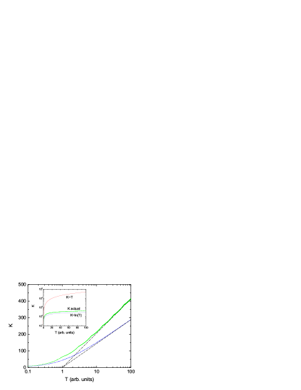
Figure 2: The number of blocks $K$ versus $T$. The dotted (blue) curve shows the optimal case given by 23. The dashed (green) curve shows the number of blocks in practice. The dot-dashed curves represent the asymptotic behaviour of the number of blocks versus time. These curves intersect the axis at $T=1$ because of the cut-off $\Delta T=1$. The inset shows the two latter quantities plotted together with the linear growth of $K$ for a typical numerical solution. The parameters in the evolution are the following: $\Delta T=1$, $d=0.016$, and $h=0.002$.

2.4 Errors

Given the blocking construction above, we can analyze how we expect the errors to behave versus both the number of blocks $K$ and the computational cost. The first question that is natural to ask is what error do we make by the replacement of the integral 11 with the approximation 15. This gives us an idea of the error incurred by keeping $K$ blocks of history in a logarithmic covering.

To answer this first we consider just the integral

$$\int_{0}^{T_{f}}\frac{e^{\imath\omega t}}{\left(t+1\right)^{p}}dt=\int_{\Delta T=1}^{T_{f}+1}\frac{e^{\imath\omega\left(t-1\right)}}{t^{p}}dt$$ (31)

where we have some frequency of oscillation $\omega$ and some power of the polynomial decay $p$. In the integration below we take $p=2$. It is important to note that in demonstrating the algorithm with just the integral 31, and not an integro-differential equation, it is not possible to show the computational speedup. However, it can show the accuracy of the integration as a function of the logarithmic coverage of the integration region when using the algorithm. We can also use it to get an idea of how the error changes when we vary $\omega$ or $p$ without having to solve the more complicated integro-differential equations. The form of this integral was chosen because of its relevance to the real-time simulation of quantum systems, where the integral of the integro-differential equation will be a sum over oscillating terms times a polynomial memory kernel.

We gave a simple error bound above. To get a better idea of errors, we can examine the behaviour of the integral 31 as a function of the blocking parameter, frequency, and the integration range (e.g., simulation time). If one takes the highest order error of the expansion 14, the worse case error in a block will occur when there is approximately one oscillation in the block,

$$b\tau_{i}=\frac{2\pi}{\omega}\,,$$ (32)

as this is when the asymmetry contributes most. However, this contribution will only occur in some finite region of the integral because the block sizes vary. When one changes the block parameter, this error will be shifted further back in time, e.g., to the left in Figure 1. The memory kernel has a smaller value at this past time, and thus the error will be decreased. If one has many frequencies contributing to the integrand, then each of their error contributions will be shifted to a later time as one decreases the block parameter. Thus, the error will be systematically reduced. The same conclusion can be drawn if one expands both the functions in the integrand around their midpoint for each block. The fractional error (the highest order error term as a fraction of the zeroth order term) in this case is

$$\frac{b^{2}}{24}\left(p(p+1)-2\imath\omega p\tau_{i}-\omega^{2}\tau_{i}^{2}\right)\,.$$ (33)

The expansion will be invalid at approximately

$$\frac{\omega^{2}b^{2}\tau_{i}^{2}}{24}\approx 1\,,$$ (34)

which gives $b\tau_{i}\sim 5/\omega$.

We compare the logarithmic covering to the midpoint method with step sizes $h=10^{-3}*2^{j}$ with $j=1,\ldots,9$. This gives a number of blocks $K_{mid}=T_{f}/h$. For the algorithm, we use a step size $h=10^{-3}$ to compute the integrals 25 and then use block parameters $b=10^{-3}*2^{j}$ with $j=1,\ldots,8$ to compute 15. The number of blocks $K_{alg}$ is then given approximately by 23. It is only approximate because each block width has to be rounded down to a multiple of $h$, this gives a larger number of blocks. We use this larger number of blocks as the value for $K_{alg}$.

If we are just looking at the integral 31, we expect the error due to the algorithm to be

$$E_{alg}\propto K_{alg}b^{3}\approx\frac{1}{K_{alg}^{2}}\left(\ln\frac{T_{f}}{\Delta T}\right)^{3}$$ (35)

so long as $bT\lessapprox 2\pi/\omega$. This can be compared to the error of the midpoint method

$$E_{mid}\propto K_{mid}h^{3}\approx\frac{T_{f}^{3}}{K_{mid}^{2}}\,.$$ (36)

Thus, if we want a fixed error, $E$, and end time, we get a difference in the number of blocks of

$$K_{mid}\propto\left(\frac{T_{f}^{3}}{E}\right)^{1/2}$$ (37)

compared to

$$K_{alg}\propto\left(\frac{\left(\ln\frac{T_{f}}{\Delta T}\right)^{3}}{E}\right)^{1/2}\,,$$ (38)

which is quite large for long times.

Figure 3 shows how the error behaves versus the number of blocks used to compute the integral. The fast decrease of error as a function of $K_{alg}$ shows that we can block together integrals as we evolve the integro-differential equation and have a controlled error. Further, the longer the simulation time, $T_{f}$, the better performing the algorithm should be when compared to the midpoint method. In addition, the overall performance of the algorithm should not be significantly affected by the frequency of integrand oscillation $\omega$ or the power $p$. One interesting feature of the error versus $K_{alg}$ figure is the slight dip in the error at approximately $bT\sim 2\pi/\omega$, which represents the error discussed above being pushed out of the integration region.

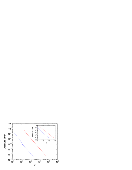
Figure 3: Absolute error versus number of blocks for the two methods of calculating the integral 31 with $\omega=2\pi$ and $p=2$ (similar curves were found for other $\omega$). The solid (red) curves are for the midpoint method and the dashed (blue) curves are for the first order blocking algorithm. The main figure shows the error for $T_{f}=100$ and the inset shows it for $T_{f}=10$. Since the midpoint method is second order, we find what is expected, $E\propto K^{-2}$. The blocking algorithm has the same dependence on $K$. The difference in error for the same number of blocks with the two methods is dependent on $T/\ln T$, reflecting the fact that the algorithm chooses blocks at optimal places and only covers the integration area with $\ln T$ blocks. We take as the exact value the one computed with a step size $h=10^{-4}$.

The second question we can ask is how the error depends on the computational cost compared to more traditional methods. If we use the method for integro-differential equations outlined in B, we have an error at each step of $h^{3}$ and we have $N$ steps. Thus

$$E_{mid}\propto Nh^{3}\propto\frac{1}{C_{pu}}\,,$$ (39)

where $C_{pu}\propto N^{2}$ is the computational cost and we hold the simulation time fixed. For the algorithm

$$E_{alg}\propto\frac{1}{C_{pu}^{2}}$$ (40)

where we hold the step size $h$ fixed and $C_{pu}=NK$. That is, the error goes down with a higher power in the computational cost.

Of course, using the algorithm is not the only way to get the error to scale better with the computational cost. One can also just block the history with constant blocks larger than $h$. Although the error does scale better, the error can never be lower than just using the brute force method, e.g., the error versus cost curve will never cross the brute force curve. For the algorithm these two curves do cross, as we will see below.

3 Examples

We consider two example problems to demonstrate the performance of the algorithm: (1) solving an integro differential equation that has both an oscillating function and a polynomially decaying function in the integral and (2) the NIBA equations for the spin-boson model.

3.1 Oscillating integro-differential equation

The oscillating integro-differential equation we use is

$$\dot{n}\left(t\right)=\imath\omega n\left(t\right)-\int_{0}^{t}dt^{\prime}\alpha\left(t-t^{\prime}\right)n\left(t^{\prime}\right)$$ (41)

with

$$\alpha(t)=\frac{1}{\left(t+1\right)^{2}}\,.$$ (42)

We get rid of the oscillation in the differential equation by setting

$$P\left(t\right)=e^{-\imath\omega t}n\left(t\right)\,,$$ (43)

which gives

$$\dot{P}\left(t\right)=-\int_{0}^{t}dt^{\prime}\alpha\left(t-t^{\prime}\right)e^{-\imath\omega\left(t-t^{\prime}\right)}P\left(t^{\prime}\right)\,.$$ (44)

This integro-differential equation involves the computation of an integral similar to 31, with $p=2$, at each time step. With the algorithm, we will be able to recycle the integral with the logarithmic covering at each step, rather than computing it from scratch. Note that we choose blocks by $b\left(t+1\right)$ here because we have the cut-off included in the polynomial decay. The simulation results for one set of parameters are shown in Figure 4.

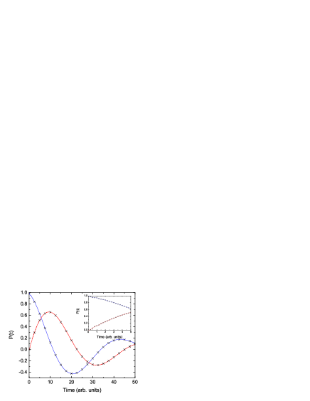
Figure 4: Real time evolution of 44 with $\omega=2\pi$. The solid (blue) curve shows the real part of $P\left(t\right)$ and the dashed (red) curve the imaginary part. These curves were calculate with the algorithm with $h=0.002$ and $d=0.016$. The crosses represent the solution using the midpoint procedure of B with a step size of $h=0.001$. The inset shows a blow up of the initial time where there is some transient structure in the solution.

Now we examine the error versus computational cost. Figure 5 is one of the main results of this paper. It shows three key results: (1) The algorithm has significantly better error for the same computational cost compared to a brute force method in a large range of parameter space. (2) As the simulation time is increased, the efficiency of the algorithm drastically increases compared to the brute force method. (3) The figure also suggests how to use the whole ansatz. Rather than have two parameters $b$ and $h$, one should set $b\propto h$ (for polynomial decay). This will give a similar convergence to the exact answer as the second order method, but a smaller factor of proportionality.

Figure 5: Absolute error versus computational cost. The error is computed by comparing the simulation results with those the brute force method with $h=0.001$ for $T_{f}=50$ (in the inset, the “exact” solution is taken as the brute method with $h=0.0002$ and $T_{f}=10$). Circles represent the brute force method for step sizes 0.1, 0.05, 0.025, 0.01, and 0.005 (in the inset, 0.1, 0.05, 0.025, 0.01, 0.005, and 0.001). The other data represents using the algorithm with the step size as shown and each data point has a different block parameter starting with $2h$ and increasing by factors of 2. For the longer simulation time of $T_{f}=50$, the algorithm has quite a substantial decrease in error for the same computational cost (for the shorter time in the inset, one can see that there is barely a gain. This is due to the overhead cost in implementing the algorithm). Also, the curves have the behaviour discussed in subsection 2.4. We perform all computations on a P4, 3 GHz processor.

As mentioned in subsection 2.4, one can also consider another method that just uses a constant grouping to reduce the number of blocks in the history. However, this method can not achieve better results as determined by the error versus computational cost. For a given step size, the highest accuracy will be achieved by using the brute procedure. A lower computational cost can be achieved by grouping the history into constant blocks, but the reduction in the computational cost will yield an even stronger loss in accuracy because $E\propto C^{-2}$, when one step size is fixed. Thus, a similar figure to Figure 5 would show curves moving only upward from the brute force line and not crossing it.

3.2 NIBA equations

The NIBA for the spin-boson model gives a good physical example for a system with a polynomially decaying kernel. The NIBA equations are derived by Leggett et al[5], see also C for a simple derivation, from which we can get the equation of motion

$$\dot{P}(t)=-\int_{0}^{t}dt^{\prime}f(t-t^{\prime})P(t^{\prime})$$ (45)

where

$$f(t)=\Delta^{2}\cos\left[2\alpha\tan^{-1}t\right]\left[\frac{\left(\pi t/\beta\omega_{c}\right)\mathrm{csch}\left(\pi t/\beta\omega_{c}\right)}{\left(1+t^{2}\right)^{1/2}}\right]^{2\alpha}\ .$$ (46)

Time is in units of the cut-off frequency $\omega_{c}^{-1}$. At zero temperature ($\beta\to\infty$) the kernel becomes

$$f(t)=\frac{\Delta^{2}\cos\left[2\alpha\tan^{-1}t\right]}{\left(1+t^{2}\right)^{\alpha}}\,.$$ (47)

The $1+t^{2}$ has a physical cut-off to the low time behaviour of the polynomial decay. There are only two parameters of interest to us. We set $\Delta=0.2$ as it is required to be small (see C) and we vary the dissipation strength $\alpha$ to see the behaviour of $P\left(t\right)$ on different sides of the dissipative transition. Varying $\alpha$ also shows the algorithm at work for different powers of polynomial decay.

Depending on the value of the dissipation strength $\alpha$, we have to use a different cut-off $\Delta T$. For $\alpha=0.5$, $1.0$, and $1.5$ we use $\Delta T=1$, $3$, and $2$, respectively. After these cut-offs, $f\left(t\right)$ is increasingly smooth (it is also smoother than bare polynomial decay). We want to point out that due to the form of the polynomial decay, the most efficient way to choose block sizes is by $b\left(1+t^{2}\right)/t$, which just comes from the inverse of the increasing smoothness. Despite this, we still use the less efficient $bt$.

The simulation results for the NIBA equations are shown in Figure 6. Using the algorithm allows one to have long simulation times for negligible computational cost. Further, simulations of NIBA-like equations on a lattice or with time dependent Hamiltonians can be done efficiently with the method.

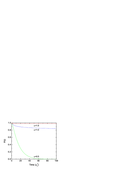
Figure 6: NIBA equations simulated in real time for $\alpha=0.5$, $1.0$, and $1.5$. The simulations were done with $h=0.008$ and $d=0.016$. They took approximately two minutes of CPU time on a P4, 3 GHz processor. This is orders of magnitude faster than a brute force approach would take to get the same error. From the figure we can clearly observe the physics of the different regimes. For weak dissipation, one gets decay to $P=0$. For the transition, $\alpha=1$, one gets $1/t^{2}$ decay of $P\left(t\right)$. Above the transition, $P\left(t\right)$ gets locked into a nonzero value.

We want to emphasize that the simulation of the NIBA equations at finite temperature 46 can also use the algorithm presented in this paper. The finite temperature, however, introduces a long-time cut-off into the kernel, beyond which the kernel may not be increasingly smooth. The contribution beyond this cut-off, though, is negligible. Thus, the algorithm can be used for times less than $\sim\beta$ exactly how it is used for the zero temperature case, and there can be a truncation of the kernel at times beyond times $\sim\beta$.

4 Conclusions

We have given an efficient and stable numerical algorithm for solving integro-differential equations with increasingly smooth memory kernels. The general computational speedup is $T^{2}\to TC\left(T\right)$, where $C\left(T\right)$ depends on how fast the kernel gets smooth. For example, the computational cost of the algorithm for polynomially decaying kernels is $T\ln T$ rather than the usual $T^{2}$.

Using a simple integro-differential equation, we demonstrated how well the algorithm performs compared to a second order, constant step size method. For long times, there is quite a substantial speedup in the computation cost to achieve a given error. The solution to the NIBA equations for the spin-boson model in real-time showed that one can get results and analyze the situation quite rapidly. Similar procedures can be applied to other forms of memory kernels which satisfy the increasingly smooth condition 7. In these other cases, the computational speedup can be better or worse than the case presented here.

In practice, the usefulness of this algorithm is due to the possibility of its incorporation into other techniques, such as matrix product state algorithms, or its use with time-dependent Hamiltonian terms. Thus, one can simulate lattices or driven systems subject to strong dissipation. The algorithm can also be used for equations less restrictive than 2, such as integro-differential equations with memory kernels dependent on both time arguments.

Appendix A Higher order blocking algorithms

The algorithm above can be extended to higher orders. For instance, if we want the next order method, we need to be able to evaluate and update

$$I^{1}\left(T,\Delta T\right)\qquad\qquad\qquad\qquad\qquad\qquad\qquad\qquad\quad$$

$$=I^{0}\left(T,\Delta T\right)+\sum_{i=1}^{K}\alpha^{\prime}\left(\tau_{i}\right)\int_{-\delta_{i}/2}^{+\delta_{i}/2}d\epsilon F\left(\tau_{i}+\epsilon,T\right)\epsilon\,.$$ (48)

The latter term picks out the asymmetric part of $F$ inside of block $i$ and then multiplies it by the derivative of $\alpha$. Lets define this asymmetric part of the block as

$$A_{i}\left(T\right)\equiv\int_{-\delta_{i}/2}^{+\delta_{i}/2}d\epsilon F\left(\tau_{i}+\epsilon,T\right)\epsilon\,.$$ (49)

If we suppose we have these asymmetric integrals at a given time, and we want to increment $T$, we first need to fix the block size, as before. Then we can update them by

$$A_{i}\left(T+h\right)=e^{-\mathcal{L}(h)}A_{i}\left(T\right)$$ (50)

We also need to be able to add these blocks together. We can do this by

$$A^{new}\left(T\right) = \int_{-B^{new}/2}^{+B^{new}/2}d\epsilon F\left(\tau^{new}+\epsilon,T\right)\epsilon$$

$$= A_{i}\left(T\right)-B_{i+1}I_{i}\left(T\right)+A_{i+1}\left(T\right)+B_{i}I_{i+1}\left(T\right)$$

where we use the asymmetric integrals from before we did the blocking and also the first order integrals 25 for the two blocks. The error for an order $z$ algorithm will have a bound proportional to $b^{z}$

Appendix B Two stage Runge-Kutta method

In this article, we compare the proposed numerical ansatz to a two stage Runge-Kutta method. Since we are dealing with integro-differential equations, we give the details of the second order technique we use. In the main text, we discuss how the errors scale with total simulation time, step size, and computational cost.

For all the examples in this work, the basic integro-differential equation 2, is reduced to

$$\frac{\partial\rho(t)}{\partial t} = \int_{0}^{t}dt^{\prime}\alpha\left(t-t^{\prime}\right)e^{-\mathcal{L}\left(t-t^{\prime}\right)}\rho\left(t^{\prime}\right)\,,$$ (52)

e.g., $\mathcal{K},\mathcal{K}^{\prime}=\mathrm{I}$. In a generic form we can write

$$\frac{\partial\rho(t)}{\partial t}=f\left[t,\rho\left(t\right),\int_{0}^{t}dt^{\prime}\mathcal{F}\left(t-t^{\prime}\right)\rho\left(t^{\prime}\right)\right]\,.$$ (53)

Discretizing time as

$$t_{n}=t_{0}+nh\,,$$ (54)

we can write a general two stage Runge-Kutta integration scheme

$$\rho_{n+1}=\rho_{n}+h\,d\rho_{n}\,,$$ (55)

$$d\rho_{n}=f\left[t,P_{n},\tilde{z}_{n}\right]\,,$$ (56)

$$P_{n}=\rho_{n}+dP_{n}\,,$$ (57)

$$dP_{n}=\frac{h}{2}f\left[t,\rho_{n},z_{n}\right]\,,$$ (58)

$$z_{n}=h\sum_{m=1}^{n-1}\bar{\mathcal{F}}_{nm}\left(\rho_{m}+\rho_{m+1}\right)/2\,,$$ (59)

and

$$\tilde{z}_{n} = h\sum_{m=1}^{n-1}\bar{\mathcal{F}}_{nm}\left(\rho_{m}+\rho_{m+1}\right)/2$$ (60)

$$+\frac{h}{2}\bar{\mathcal{F}}_{0}\left(\rho_{n}+P_{n}\right)/2\,,$$

where

$$\bar{\mathcal{F}}_{nm}=\frac{1}{h}\langle\mathcal{F}\left(t_{n}-t^{\prime}\right)\rangle_{t_{m}}^{t_{m}+h}=\frac{1}{h}\int_{t_{m}}^{t_{m}+h}dt^{\prime}\mathcal{F}\left(t_{n}-t^{\prime}\right)$$ (61)

and

$$\bar{\mathcal{F}}_{0}=\frac{2}{h}\int_{t_{n}-h/2}^{t_{n}}dt^{\prime}\mathcal{F}\left(t_{n}-t^{\prime}\right)\,.$$ (62)

Although using the average $\bar{\mathcal{F}}_{nm}$ over an interval does not increase the order of the method, it does preserve important properties of the kernel such as its total integration. This is very important in cases where the kernel integrates to zero and thus the transient behaviour completely determines the steady state. We use the average of the kernel over each block with the algorithm as well. The Runge-Kutta scheme can of course be generalized to higher stages and to kernels with two time arguments.[16, 17, 18, 19]

Appendix C Simple derivation of the NIBA equations

In this appendix we give a simple derivation of the NIBA equations for the spin-boson model to show how polynomially decaying memory kernels can arise physically in the case of strong dissipation. The derivation of the NIBA equations is based on the observation that they come from a Born approximation of a transformed Hamiltonian.[20]

The spin-boson Hamiltonian is

$$H_{SB}=-\frac{1}{2}\Delta\sigma_{x}+\frac{1}{2}\epsilon\sigma_{z}+\sum_{k}\omega_{k}a_{k}^{\dagger}a_{k}+\gamma\sigma_{z}\sum_{k}g_{k}\left(a_{k}^{\dagger}+a_{k}\right)$$ (63)

where we have a two level system with internal coupling constant $\Delta$ and bias $\epsilon$. The two level system is coupled to an collection of bosons of frequencies $\left\{\omega_{k}\right\}$ with a coupling constant $g_{k}=c_{k}/\sqrt{2m_{k}\omega_{k}}$ and overall coupling factor $\gamma$. The spectral density of the bath is given by

$$J\left(\omega\right)=\pi\sum_{k}g_{k}^{2}\delta\left(\omega-\omega_{k}\right)\,.$$ (64)

The physical scenario we want to explore is one in which the two level system is initially held fixed in an eigenstate of $\sigma_{z}$ while the bath equilibrates around this state. That is, the bath will equilibrate around the Hamiltonian

$$H_{R}=\sum_{k}\omega_{k}a_{k}^{\dagger}a_{k}+\sum_{k}\gamma g_{k}\left(a_{k}^{\dagger}+a_{k}\right)$$ (65)

if we hold the two level system in the $+1$ eigenstate of $\sigma_{z}$. This gives the thermal starting state for the bath

$$R_{0}=\frac{e^{-\beta H_{R}}}{Z_{R}}\,.$$ (66)

Then, we want to release the two level system and follow its dynamics in real time. In particular, we look at the expectation value of $\sigma_{z}$

$$P\left(t\right) \equiv \langle\sigma_{z}\rangle_{t}$$ (67)

$$= \tr\left\{e^{\imath H_{SB}t}\sigma_{z}e^{-\imath H_{SB}t}|1\rangle\langle 1|\otimes R_{0}\right\}\,.$$ (68)

Since we are interested in strong dissipation, we can perform a canonical transformation on this Hamiltonian to incorporate all orders of the system-bath interaction. With

$$S=-\sum_{k}\frac{\gamma g_{k}}{\omega_{k}}\left(a_{k}-a_{k}^{\dagger}\right)\sigma_{z}$$ (69)

we get

$$H = e^{S}H_{SB}e^{-S}$$ (70)

$$= -\frac{1}{2}\Delta\left(\sigma_{+}B_{-}+\sigma_{-}B_{+}\right)+\frac{1}{2}\epsilon\sigma_{z}+\sum_{k}\omega_{k}a_{k}^{\dagger}a_{k}$$ (71)

where

$$B_{\pm}=\exp\left\{\pm 2\sum_{k}\frac{\gamma g_{k}}{\omega_{k}}\left(a_{k}-a_{k}^{\dagger}\right)\right\}\,.$$ (72)

For the unbiased case, $\epsilon=0$, this gives the interaction picture Hamiltonian

$$H^{I}\left(t\right)=-\frac{1}{2}\Delta\left(\sigma_{+}B_{-}^{I}\left(t\right)+\sigma_{-}B_{+}^{I}\left(t\right)\right)$$ (73)

with

$$B_{\pm}^{I}\left(t\right)=\exp\left\{\pm 2\sum_{k}\frac{\gamma g_{k}}{\omega_{k}}\left(a_{k}e^{-\imath\omega_{k}t}-a_{k}^{\dagger}e^{\imath\omega_{k}t}\right)\right\}\,.$$ (74)

We can then transform the equation for $P\left(t\right)$ to get

$$P\left(t\right) = \tr\left\{e^{\imath Ht}\sigma_{z}e^{-\imath Ht}|1\rangle\langle 1|\otimes R_{0}^{\prime}\right\}$$ (75)

where

$$R_{0}^{\prime}=e^{-\beta\sum_{k}\omega_{k}a_{k}^{\dagger}a_{k}}/Z_{R}^{\prime}\,.$$ (76)

We can find the master equation in the Born approximation for $P\left(t\right)$, also known as the noninteracting blip approximation, by performing perturbation theory on 75. To second order in $\Delta$,

$$\dot{P}(t)=-\int_{0}^{t}dt^{\prime}f(t-t^{\prime})P(t^{\prime})$$ (77)

with

$$f\left(t\right) = \frac{\Delta^{2}}{4}\left\{\langle\left[B_{+}^{I}\left(t\right),B_{-}^{I}\left(0\right)\right]\rangle_{R_{0}^{\prime}}\right.$$ (78)

$$\left.+\langle\left[B_{+}^{I}\left(-t\right),B_{-}^{I}\left(0\right)\right]\rangle_{R_{0}^{\prime}}\right\}$$

$$= \frac{\Delta^{2}}{2}\langle\left[B_{+}^{I}\left(t\right),B_{-}^{I}\left(0\right)\right]\rangle_{R_{0}^{\prime}}$$ (79)

where we have used that the correlation functions are equal. To compute $f\left(t\right)$ we can use the Feynman disentangling of operators [21] to get, in the notation of Leggett et al[5],

$$f\left(t\right)=\Delta^{2}\cos\left\{\frac{4\gamma^{2}}{\pi}Q_{1}\left(t\right)\right\}\exp\left\{-\frac{4\gamma^{2}}{\pi}Q_{2}\left(t\right)\right\}$$ (80)

with

$$Q_{1}\left(t\right)=\int_{0}^{\infty}d\omega\frac{J\left(\omega\right)}{\omega^{2}}\sin\left(\omega t\right)$$ (81)

and

$$Q_{2}\left(t\right)=\int_{0}^{\infty}d\omega\frac{J\left(\omega\right)}{\omega^{2}}\left(1-\cos\omega t\right)\coth\left(\frac{\beta\omega}{2}\right)\,.$$ (82)

For ohmic dissipation, $J\left(\omega\right)=\eta\omega\exp\left(-\omega/\omega_{c}\right)$, these quantities become

$$Q_{1}\left(t\right)=\eta\tan^{-1}\omega_{c}t$$ (83)

and

$$Q_{2}\left(t\right)=\frac{\eta}{2}\ln\left(1+\omega_{c}^{2}t^{2}\right)+\eta\ln\left(\frac{\beta}{\pi t}\sinh\frac{\pi t}{\beta}\right)\,.$$ (84)

With $\alpha\equiv 2\eta\gamma^{2}/\pi$, this gives 46 for the NIBA memory kernel.

References

References

- [1] Feynman R P and Vernon F L 1963, Ann. Phys. - New York 24 118
- [2] Keldysh L V 1965 Sov. Phys. JETP 20 1018
- [3] Kadanoff L P and Baym G 1962 Quantum Statistical Mechanics (W. A. Benjamin, Inc., New York)
- [4] Breuer H -P and Petruccione F 2002 The Theory of Open Quantum Systems (Oxford University Press, Oxford)
- [5] Leggett A J, Chakravarty S, Dorsey A T, Fisher M P A, Garg A, and Zwerger W 1987 Rev. Mod. Phys. 59 1
- [6] Schön G and Zaikin A D 1990 Phys. Rep. 198 237
- [7] Cushing J M 1977 Integrodifferential equations and delay models in population (Springer-Verlag, Berlin)
- [8] Zwolak M and Vidal G 2004 Phys. Rev. Lett. 93 207205
- [9] Verstraete F, Garcia-Ripoll J J, and Cirac J I 2004 Phys. Rev. Lett. 93 207204
- [10] Vidal G 2003 Phys. Rev. Lett. 91 147902
- [11] Vidal G 2004 Phys. Rev. Lett. 93 040502
- [12] Zwolak M and Refael G 2007 in preparation
- [13] Shabani A and Lidar D A 2001 Phys. Rev. A 71 020101(R)
- [14] Barnett S M and Stenholm S 2001 Phys. Rev. A 64 033808
- [15] Daffer S, Wódkiewicz K, Cresser J D, and Mclver J K 2004 Phys. Rev. A 70 010304(R)
- [16] Leathers A S and Micha D A 2005 Chem. Phys. Lett. 415 46
- [17] Brunner H and van der Houwen P J 1986 The Numerical Solution of Volterra Equations (North-Holland, New York)
- [18] Linz P 1985 Analytical and Numerical Methods for Volterra Equations (SIAM, Philadelphia)
- [19] Lubich Ch 1982 Numer. Math. 40 119
- [20] Aslangul C, Pottier N, and Saint-James D 1986 J. Physique 47 1657
- [21] Mahan G 2000 Many-Particle Physics (Kluwer Academic/Plenum Publishers, New York)