Characterization of Disorder in Semiconductors via Single–Photon Interferometry

Abstract

The method of angular photonic correlations of spontaneous emission is introduced as an experimental, purely optical scheme to characterize disorder in semiconductor nanostructures. The theoretical expression for the angular correlations is derived and numerically evaluated for a model system. The results demonstrate how the proposed experimental method yields direct information about the spatial distribution of the relevant states and thus on the disorder present in the system.

Disorder in solids is a topic of increasing interest in solid-state research in the last decades. Intriguing and widely celebrated phenomena likeQuantum-Hall-Effect, photon echoes, and Anderson localization rely on the existence of disorder. However, the significance of disorder is not purely academic. Modern devices are fabricated on smaller and smaller length scales. Systems with reduced dimensionality can be realized by semiconductor heterostructures. Concomitantly, disorder due to interface roughness and/or compositional fluctuations plays a crucial role in the performance of these nanostructures. Clearly, for a detailed understanding of the influence of disorder on the investigated phenomena, it is important to know to what degree the electronic states deviate from the Bloch-like character which governs the electronic properties in perfectly periodic structures. In particular, localized electronic states can occur which strongly alter both the optical and transport properties of a given system ot ; es ; ei ; mtk ; Yayon:PRL ; hardToMapDisorderToOptics-1 ; hardToMapDisorderToOptics-2 . It is, therefore, important to have a reliable method that allows the experimentalist to quantitatively characterize the disorder in a given structure without its destruction. Unfortunately, in this respect the present situation is not very satisfactory.

For example, the lattice disorder in alloy semiconductors can be determined in principle by spatially resolved atomic–level microscopies nature ; nature-afm ; nature-stm ; nature-stm2 ; nature-tem , but its influence on e.g. optical properties is still not well understood Yayon:PRL ; hardToMapDisorderToOptics-1 ; hardToMapDisorderToOptics-2 . Alternatively, one can obtain information about the connection of disorder and optical properties directly within the resolution limit set by the wavelength of light. Examples include micro-(nano)-luminescence wegener-1 ; wegener-2 , near-field optical imaging nr4-1 ; nr4-2 , and resonant Rayleigh scattering (RRS) schwedt2006 ; resram ; Langbein:PRL2002 . In order to deduce the spatial dependence of the disorder potential, the first two methods require a spatial scanning of the sample. When the angular dependence of the RRS intensity is measured, one can determine the energy statistics of emitters resram , as well as the localization length scales of the optically active excitonic states schwedt2006 ; resram ; Langbein:PRL2002 . However, RRS can deduce the exact disorder potential and position of emitters only indirectly via an inverse-scattering problem.

In this Letter, we suggest a quantum–optical interferometric method which provides the disorder potential directly. Our scheme is based on the photonic correlations that are determined from the stationary spontaneous emission by collecting two different emission directions into a common detector. Recent experiments have shown that strong single–photon interferences can be observed in this setup walter . We demonstrate that the qualitative features of these interferences can be utilized to reconstruct the disorder landscape of the light emitters for length scales varying between the used wavelength and the illumination spot size. We also show that the reconstruction of disorder potential can be performed solely on the basis of experimental data and that the method is robust to experimental inaccuracies. In contrast with micro-(nano)-luminescence wegener-1 ; wegener-2 and near-field optical imaging nr4-1 ; nr4-2 , our scheme does not need spatial scanning.

To present the idea behind our proposed quantum–optical method, we need to quantize the light field and compute the correlations among the emitted photons including the disorder as well as the relevant many–body interactions among the electron–hole excitations in the semiconductor heterostructure. For this purpose, and in order to keep our analysis as transparent as possible, we choose a simple model based on a one–dimensional tight–binding description. For a chain of $N$ sites with periodic boundary conditions, every site, if isolated from the others, supports one electron and one hole state with the energies $\epsilon_{j}^{e}$ and $\epsilon_{j}^{h}$, respectively. The index $j$ refers to the position of the site and the energies $\epsilon_{j}^{e,h}$ vary from site-to-site due to disorder. The corresponding carrier system is described by the material Hamiltonian

$${H}_{\mathrm{mat}} = \sum_{j}\epsilon_{j}^{e}e^{{\dagger}}_{j}e_{j}+J^{e}\sum_{<jl>}e^{{\dagger}}_{j}e_{l}+\sum_{j}\epsilon_{j}^{h}h^{{\dagger}}_{j}h_{j}$$ (1)

$$+ J^{h}\sum_{<jl>}h^{{\dagger}}_{j}h_{l}-\sum_{j,l}V_{jl}\,e^{{\dagger}}_{j}h^{{\dagger}}_{l}h_{l}e_{j}$$

where $e^{{\dagger}}_{j},e_{j}$ and $h^{{\dagger}}_{j},h_{j}$ denote the electron and hole creation and annihilation operators at a site $j$. The constant $J^{e,h}$ defines the bandstructure via the nearest neighbor coupling indicated by the symbol $<jl>$. We concentrate here on low–density conditions such that we only describe the attractive Coulomb interaction of electron–hole pairs, given by the last term in Eq. (1). The model parameters are chosen to reproduce the effective mass and the exciton binding energy of typical GaAs quantum–well systems mtk . In particular, $N$ sites are positioned evenly at distances $a$ with $J^{e}=-5.737$ meV and $J^{h}=0.835$ meV. The regularized Coulomb matrix element is given by $V_{jl}=U_{0}/(|j-l|a+a_{0})$ with $U_{0}=7$ meV and $a_{0}=0.5\,a$. This yields an exciton binding energy of $E_{b}=7.5$ meV.

The quantized light field can be expressed via a mode expansion in terms of plane–wave modes $u_{\mathbf{q}}{\left(\mathbf{r}\right)}=e^{i\mathbf{q}\cdot\mathbf{r}}$ with momenta $\mathbf{q}$ cohen ; PQE and photon operators $B_{\mathbf{q}}$. The light–matter interaction is given by ${H}_{\mathrm{L}}={\sum_{\mathbf{q}}\hbar\omega_{q}(B_{\mathbf{q}}^{{\dagger}}B_{\mathbf{q}}+1/2)}-\sum_{\mathbf{q},j}({i\eta u_{\mathbf{q},j}B_{\mathbf{q}}e^{\dagger}_{j}h^{\dagger}_{j}+\mathrm{h.c.}})$, where the absorption of a photon creates an electron–hole pair at the site $j$ since only direct transitions are allowed. This term is proportional to $\eta=\mu_{0}{\mathcal{E}}$ with the dipole–matrix element $\mu_{0}$ and the vacuum–field amplitude ${\mathcal{E}}$. The light–matter interaction also depends on the mode function $u_{\mathbf{q},j}$ at the position of the site, $\mathbf{R}_{j}$. The sites can be assummed to be equally spaced since their size is much smaller than the optical wavelength. Consequently, we may choose $\mathbf{R}_{j}=R_{j}\mathbf{e}_{\|}=aj\mathbf{e}_{\|}$ such that all disorder effects enter via the energies $\epsilon^{e,h}_{j}$. The corresponding $u_{\mathbf{q},j}=e^{iR_{j}q_{\|}}$ contains the in-plane photon momentum in the direction $\mathbf{e}_{\|}$.

Under incoherent conditions, all coherent quantities, $\langle h_{j}e_{j}\rangle$, $\langle e_{j}^{\dagger}h_{j}^{\dagger}\rangle$ and $\langle B_{\mathbf{q}}\rangle$ , $\langle B_{\mathbf{q}}^{\dagger}\rangle$, vanish. In this situation, the system emits light only spontaneously leading to non–vanishing $\langle{B_{\mathbf{q}}}^{\dagger}B_{\mathbf{q^{\prime}}}\rangle$. For steady–state conditions, the photon–flux $\partial/{\partial t}\langle B_{\mathbf{q}}^{\dagger}B_{\mathbf{q}}\rangle$ defines the photoluminescence (PL) intensity while $\partial/{\partial t}\langle B_{\mathbf{q}}^{\dagger}B_{\mathbf{q}^{\prime}}\rangle$ determines the quantum-optical correlations between two different emission directions. By using a suitable optical arrangement, one can collect light in the directions $\mathbf{q}$ and $\mathbf{q}^{\prime}\neq\mathbf{q}$ to a common detector. With this interferometric setup, $U_{\mathbf{q},\mathbf{q}^{\prime}}\equiv\partial/{\partial t}\langle B_{\mathbf{q}}^{\dagger}B_{\mathbf{q}^{\prime}}\rangle$ defines the contrast of the single–photon interferences walter for steady–state emission conditions. This quantity follows from

$$\hbar U_{\mathbf{q},\mathbf{q}^{\prime}}=-\sum_{l}\left({\eta^{*}u_{\mathbf{q^{\prime}},l}^{*}}{}\Pi^{\mathbf{q}}_{l,l}+{\eta u_{\mathbf{q},l}}{\Pi^{\mathbf{q^{\prime}}}_{l,l}}^{*}\right)\,,$$ (2)

showing that $U_{\mathbf{q},\mathbf{q}^{\prime}}$ is coupled to the photon–assisted polarization $\Pi^{\mathbf{q}}_{j,l}\equiv\langle B^{\dagger}_{\mathbf{q}}h_{j}e_{l}\rangle$ and its dynamics

$$i\hbar\frac{\partial}{\partial t}\Pi^{\mathbf{q}}_{j,l}=\left(\epsilon_{j,l}-\hbar\omega_{q}\right)\Pi^{\mathbf{q}}_{j,l}+J^{e}\sum_{\Delta=\pm 1}\Pi^{\mathbf{q}}_{j,l+\Delta}$$

$$+J^{h}\sum_{\Delta=\pm 1}\Pi^{\mathbf{q}}_{j+\Delta,l}+i\hbar\frac{\partial}{\partial t}\Pi_{j,l}^{\mathbf{q}}|^{\mathrm{scatt}}+i\hbar\frac{\partial}{\partial t}\Pi_{j,l}^{\mathbf{q}}|^{\mathrm{stim}}$$

$$-V_{lj}\left(1-f_{j}^{h}-f_{l}^{e}\right)\Pi^{\mathbf{q}}_{j,l}+i\eta u_{\mathbf{q},j}S_{jl}\,\,,$$ (3)

where $\epsilon_{j,l}=\epsilon_{l}^{e}+\epsilon_{j}^{h}-\sum_{m}\left(V_{lm}f_{m}^{e}+V_{jm}f_{m}^{h}\right)$. The second line in Eq. (3) contains contributions due to Coulomb scattering and stimulated emission. The stimulated term can be omitted for systems without a cavity PQE . As another simplification, we introduce a constant dephasing $\hbar\frac{\partial}{\partial t}\Pi_{j,l}^{\mathbf{q}}|^{\mathrm{scatt}}=-\gamma\Pi_{j,l}^{\mathbf{q}}$. When the carrier system is in a quasi-equilibrium, $S_{jl}=\sum_{m}u_{\mathbf{q},m}/u_{\mathbf{q},j}\langle e_{m}^{{\dagger}}h_{m}^{{\dagger}}h_{j}e_{l}\rangle$ acts as a constant spontaneous–emission source and the Coulomb term, $V\Pi$, leads to excitonic resonances in the emission. At the lowest level, $S_{jl}$ is given by its Hartree–Fock approximation $S_{jl}=\delta_{jl}f_{j}^{e}f_{j}^{h}$ containing the excited state occupations, $f_{j}^{e}=\langle e_{j}^{\dagger}e_{j}\rangle$ and $f_{j}^{h}=\langle h_{j}^{\dagger}h_{j}\rangle$.

In order to understand how disorder effects enter in $U_{\mathbf{q},\mathbf{q}^{\prime}}$, we first solve Eqs. (2)–(Characterization of Disorder in Semiconductors via Single–Photon Interferometry ) for a simplified case by setting all carrier–interaction terms to zero $J^{e,h}_{j}=V_{jl}=0$. This yields a steady–state expression

$$U_{\hbar\omega}(\Delta q)\equiv U_{{\mathbf{q}},{\mathbf{q}^{\prime}}}={\mathcal{N}}\sum_{j}\frac{\gamma S_{jj}e^{i\Delta qR_{j}}}{\left(\epsilon_{j}-\hbar\omega_{q}\right)^{2}+\gamma^{2}}\,\,,$$ (4)

where $\epsilon_{j}=\epsilon^{e}_{j}+\epsilon^{h}_{j}$. We have also assumed that $\left|\mathbf{q}\right|=\left|\mathbf{q}^{\prime}\right|$ differ only by the emission direction giving $\omega=c\left|\mathbf{q}\right|$ and $\Delta q=q_{\|}-q_{\|}^{\prime}$. The normalization $\mathcal{N}$ is chosen such that the correct $100\%$ interference contrast is observed for $\mathbf{q}=\mathbf{q}^{\prime}$. This form clearly shows that even the spontaneous emission contains a phase, $e^{i\Delta qR_{j}}$, influenced by the position of the emitters. This phase can always be observed as single–photon interferences walls , which is the fundamental principle behind the proposed interferometry.

In the continuum limit $a\rightarrow 0$, Eq. (4) reduces to

$$U_{\hbar\omega}\left(\Delta q\right)={\mathcal{N}}\int\frac{\gamma S(x)}{\left(\epsilon(x)-\hbar\omega\right)^{2}+\gamma^{2}}e^{i\Delta qx}dx\,,$$ (5)

where $S(x)$ defines the level of excitation. We now notice that Fourier transformation of Eq. (5) with respect to $\Delta q$ produces a peak at $\epsilon(x)=\hbar\omega$; i.e. the position of the emitters can be determined. Thus we define

$$U_{\hbar\omega}(x)=\int_{-\Delta q_{0}}^{\Delta q_{0}}U_{\hbar\omega}\left(\Delta q\right)e^{-i\Delta qx}d\Delta q,$$ (6)

where $\Delta q_{0}=2\omega/c=4\pi/\lambda_{0}$ is the largest in-plane momentum which is accessible in principle. This allows us to reconstruct the disorder potential up to the limits set by $\Delta q_{0}$ via

$$U(x)={\int_{E_{1}}^{E_{2}}\hbar\omega\left|U_{\hbar\omega}(x)\right|d\hbar\omega}/{\int_{E_{1}}^{E_{2}}\left|U_{\hbar\omega}(x)\right|d\hbar\omega}\,.$$ (7)

The integration limits are set by the relevant spectral range $E_{1}<\hbar\omega<E_{2}$. Equations (6)–(7) suggest a general interferometric scheme to determine the disorder landscape. First, the interference contrast $U_{\hbar\omega}\left(\Delta{q}\right)$ has to be measured as function of energy for different emission directions. Second, a simple Fourier transform of $U_{\hbar\omega}\left(\Delta{q}\right)$ produces directly the disorder landscape of emitters.

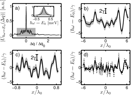
Figure 1: a) Correlation function $U_{\hbar\omega=E_{0}}(\Delta q)$ as a function of $\Delta q/\Delta q_{0}$ for noninteracting TLS. The inset shows PL for the ordered (line) and the disordered (shaded) case. b) Contour plot of the spatially dependent correlation function $U_{\hbar\omega}(x)$. Solid line is the input potential with ${\cal L}=1.2\lambda_{0}$. c) The same for the fully interacting system, ${\cal L}=0.2\lambda_{0}$. $E_{b}$ is the sum of $E_{0}$ and the binding energy. d) Dashed line: input potential with ${\cal L}=0.25\lambda_{0}$, based on the same initial distribution of site energies for noninteracting TLS as b). Solid line: $U(x)$, c.p. with solid line in b).

In our full numerical computations, we generate the energies $\epsilon_{j}^{e}$ and $\epsilon_{j}^{h}$ from a random box–like distribution of width $W^{e}$ and $W^{h}$, respectively. We take $W^{e}/W^{h}=|J^{e}/J^{h}|$, which guarantees that the disorder amplitudes scale with the effective masses. The ordered case is recovered by setting $W^{e}=W^{h}=0$, i.e., $\epsilon_{j}^{e,h}=\epsilon^{e,h}$. The length scale of the disorder potential $\cal L$ is defined by a Gaussian low–pass filter applied in Fourier space with a maximum spatial frequency $\propto{\cal L}^{-1}$. We use $\lambda_{0}=800$ nm, band gap energy $E_{0}=1.5$ eV, $\gamma=0.1$ meV, $N=2048$, and $a=5$ nm.

To illustrate the single–photon interferometric scheme, we first consider the non-interacting case and set the excitation $S(x)$ to a constant value within a 10 $\mu$m excitation spot. The inset in Fig. 1a shows the photoluminescence for $W^{e}=0.5$ meV (shaded area) and the ordered case (solid line); clear inhomogeneous broadening is observed. The interference contrast, $U_{\hbar\omega}\left(\Delta q\right)$ is presented in Fig. 1a for $\hbar\omega=E_{0}$ as function of $\Delta q$. The central peak at $\Delta q=0$ produces a 100% interference constrast while $U$ drops quickly for elevated $\left|\Delta q\right|$. The peak structure at small $\left|\Delta q\right|$ values contains direct information about the disorder. The width of both central and side peaks is $2\pi/\cal{S}$ where $\cal{S}$ is the size of the spot. After $U_{\hbar\omega}\left(\Delta q\right)$ is defined for all relevant frequencies, we may construct $U_{\hbar\omega}(x)$ via Eq. (6). We use the maximum optically allowed $\Delta q$ (denoted by shaded area in Fig. 1a) as the integration limits. The generated $U_{\hbar\omega}\left(x\right)\geq\frac{1}{2}$ contour is shown in Fig. 1b as shaded area, denoting the full width of half maximum of $U_{\hbar\omega}\left(x\right)$, while the original potential is given by the solid line. Clearly the center of $U_{\hbar\omega}(x)$ reproduces excellently the $x$ dependence of the actual disorder landscape. For a fixed $x$, $U_{\hbar\omega}(x)$ gives the homogeneous line for the $\mu$PL spectrum of the emitter at position $x$. In the present paper, this width is determined by the constant $\gamma$. In reality, microscopic carrier and phonon scattering can lead to a position dependent homogeneous line width which should be observable in the same way. The total inhomogeneous spectrum follows as an integral over $x$. In Fig. 1d we show results for a disorder potential with ${\cal L}=0.25\lambda_{0}$. The long-range features of this potential are very well reproduced by our method.

From an experimental point of view it is critical to know i) the range of $\mathbf{q}$-vectors which can be detected and ii) how accurately the side peaks of $U$ must be measured with respect to the central peak. Concerning i), the experimental setup from Ref. schwedt2006 would allow for a range of $\Delta q=N.A./n_{GaAs}\simeq 0.12\Delta q_{0}$ only (N.A. is the numerical aperture). Augmenting the setup by a solid state immersion lens with high index of refraction (for a discussion see barnes2002 ), and using two optimal positioned microscope objectives $\Delta q\simeq\pm 0.85\Delta q_{0}$ can be achieved. This range is indicated by the shaded area in Fig. 1a. Concerning ii), we have solved Eq. (5) analytically for a sinusoidal $\epsilon(x)$. In particular, we find that the second peak of $U_{\hbar\omega}\left(\Delta q\right)$ is located at $\Delta q=4\pi/\cal{L}$ and the ratio $r$ between the central peak and the second one is $r_{\mathrm{sin}}=(\sqrt{1+(\gamma/{\Delta}W)^{2}}+\gamma/{\Delta}W)^{-2}$, where ${\Delta}W$ is the standard deviation of the potential. Taking two sinusoidal functions with equal amplitude but different spatial frequency yields values for $r$ situated clearly below $r_{\mathrm{sin}}$. For various random potentials, we find $r$ is around $r_{\mathrm{sin}}/2$. This analysis shows that the ratio $\gamma/{\Delta}W$ defines the accuracy requirements in an experiment. For example, if one wants to resolve disorder up to ${\Delta}W>\gamma/2$, one has to measure the interference contrast with 10% accuracy.

To verify the general validity of the scheme defined by Eqs. (6)–(7), we next investigate the fully interacting case by including the band–structure, disorder, and Coulomb interaction terms in Eq. (Characterization of Disorder in Semiconductors via Single–Photon Interferometry ). We solve the eigenstates $\Phi_{jl}^{\lambda}$ and eigenvalues $\epsilon_{\lambda}$ of the homogeneous part of Eq. (Characterization of Disorder in Semiconductors via Single–Photon Interferometry ) for steady–state conditions. This procedure yields peter1

$$U_{\hbar\omega}\left(\Delta q\right)=\sum_{\lambda,jl}\frac{\gamma{\mathcal{N}}\Phi_{jj}^{\lambda}\Phi_{ll}^{\lambda}e^{i{\Delta q}\left(R_{j}+R_{l}\right)/2}}{\left(E_{\lambda}-\hbar\omega\right)^{2}+\gamma^{2}}\,\,,$$ (8)

for constant $S$. We evaluate Eq. (8) numerically for a disorder realization with $W=5\gamma$. Since our main purpose is to show that the interaction contributions do not affect the reconstruction procedure (6)–(7), we can restrict the calculations to a rather small system ($N=140$, $a=10$ nm) to obtain numerically feasible computations. Physically, this implies a small ${\cal S}=1.4\,\mu$m spotsize. Numerically, this leads to a relatively large discretization in $\Delta q$ which forces us to use the $\Delta q$ data taken from the entire Brillouin zone in the reconstruction procedure. Figure 1c shows the obtained full $U_{\hbar\omega}\left(x\right)\geq\frac{1}{2}$ in a contour plot (shaded area) and compares it with the actual potential (solid line) note . Again, the center of $U_{\hbar\omega}(x)$ matches well with the original disorder potential, which demonstrates the general applicability and the robustness of the proposed scheme.

To determine the sensitivity of the reconstruction procedure on several experimentally relevant inaccuracies, we apply Eq. (5) to reconstruct the potential via Eq. (7) for different situations of the non–interacting case. In all frames of Fig. 2 the shaded area indicates the original potential with $W=5\gamma$ and the reconstructed potential $U(x)$ is shown as a solid line. In Fig. 2a, $U_{\hbar\omega}(x)$ is constructed by omitting values of $U_{\hbar\omega}\left(\Delta q\right)$ with interference contrast below 10%. In Fig. 2b, $U_{\hbar\omega}(x)$ is constructed from $U_{\hbar\omega}\left(\Delta q\right)$ where we simply added a 5% random noise. When the momentum scan is limited to $\left|\Delta q\right|<\Delta q_{0}/2$ and $\left|\Delta q\right|<2\Delta q_{0}$ (dashed line) we obtain the $U_{\hbar\omega}(x)$ results presented in Fig. 2c. This is also accompanied by a limitation of the spatial resolution of the resulting reconstructed potential. For a minimum $\Delta q_{\mathrm{min}}$ given by experimental limitations, the spot size should be chosen accordingly, such that $S=2\pi/\Delta q_{\mathrm{min}}$ in order to avoid aliasing problems.

All these cases indicate that the proposed photon–correlation interferometry produces the disorder potential even when a reasonable amount of experimental inaccuracies are present.

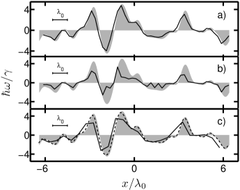
Figure 2: Sensitivity of the reconstructed potential to various external parameters: a) sensitivity of measurement of the interference contrast, b) random noise, and c) range of momentum scan. Details are in the text.

In conclusion, we suggest that the experimental method of single–photon interferometry can directly characterize the optically relevant disorder landscape in semiconductor heterostructures. The method is only limited by the wavelength of light and the optical spotsize. We have also demonstrated a remarkable quality of the reconstructed potential even for weak disorder and added random noise.

- (1) H. Overhof and P. Thomas, “Electronic Transport in Hydrogenated Amorphous Semiconductors”, Springer Tracts in Mod. Phys., Vol. 114 (Springer, Berlin, 1989)
- (2) B. I. Shklovskii and A. L. Efros, “Electronic Properties of Doped Semiconductors”, Springer, Heidelberg (1984).
- (3) “Optical Properties of Mixed Crystals”, Ed. R. J. Elliott and I. P. Ipatova, Elsevier, (1988)
- (4) T. Meier, P. Thomas, and S. W. Koch, “Coherent Semiconductor Optics: From Basic Concepts to Nanostructure Applications”, Springer-Verlag, in print
- (5) Y. Yayon et.al., Phys. Rev. Lett. 89, 157402 (2002)
- (6) C. Ell et.al., Phys. Rev. Lett. 80, 4795 (1998)
- (7) A. V. Shchegrov et.al., Phys. Rev. Lett. 84, 3478 (2000)
- (8) A. Yazdani, C. M. Lieber, Nature, 401, pp. 227 (1999)
- (9) U. Banin et.al., Nature, 400, pp. 542 (1999)
- (10) C. Renner et.al., Nature, 416, pp. 518 (2002)
- (11) P. Zhang et.al., Nature, 439, pp. 703 (2006)
- (12) C. Barth and M. Reichling, Nature 414, pp. 54 (2001)
- (13) U. Neubert et al., Appl. Phys. Lett. 80, 3340 (2002)
- (14) G. von Freymann et al., Phys. Rev. B65, 205327 (2002)
- (15) A. Richter et al., Phys. Rev. Lett. 79, 2145 (1997)
- (16) R. Cingolani et al., J. of Appl. Phys. 86, 6793 (1999)
- (17) D. Schwedt et.al., phys. stat. solidi (c), in press (2006)
- (18) R. Zimmermann, E. Runge, and V. Savona, in “Quantum Coherence, Correlation and Decoherence in Semiconductor Nanostructures”, (Ed. Toshihide Takagahara), Elsevier Science (USA), p. 89-165 (2003)
- (19) W. Langbein et.al., Phys. Rev. Lett. 89, 157401 (2002)
- (20) W. Hoyer et.al., Phys. Rev. Lett. 93, 067401 (2004)
- (21) C. Cohen-Tannoudji, J. Dupont-Roc, G. Grynberg, Photons & Atoms, 3rd Edition, Wiley, New York, (1989)
- (22) M. Kira, et.al., Prog. in Quant. Electr. 23, 189 (1999)
- (23) D. F. Walls, G. J. Milburn, “Quantum Optics” (Springer, Berlin, Heidelberg, 1994)
- (24) W.L. Barnes et.al., Eur. Phys.J. D 18, 197 (2002)
- (25) P. Bozsoki et al., J. of Luminescence, in press (2006)
- (26) The reconstruction of features smaller than is a direct consequence of our integration over the whole Brillouin zone and will not be observed in an experiment.