Molecular Conductance from Ab Initio Calculations: Self Energies and Absorbing Boundary Conditions

Abstract

Calculating an exact self energy for ab initio transport calculations relevant to Molecular Electronics can be troublesome. Errors or insufficient approximations made at this step are often the reason why many molecular transport studies become inconclusive. We propose a simple and efficient approximation scheme, that follows from interpreting the self energy as an absorbing boundary condition of an effective Schrödinger equation. In order to explain the basic idea, a broad introduction into the physics incorporated in these self energies is given. The method is further illustrated using a tight binding wire as a toy model. Finally, also more realistic applications for transport calculations based on the density functional theory are included.

1 Introduction

The most important driving force in the research field of Molecular Electronics are prospects on technological applications – whence the name – in entirely new realms of system parameters likharev03 . The development of these new technologies also requires serious progress in several disciplines of fundamental sciences including both, theory and experiment. One of the major theoretical challenges is the quantitative description of transport through a molecule with a given contact geometry reimers03 ; evers03prb ; kurth:035308 ; sai05 ; burke05a .

In order to appreciate the caliber of the problem, recall that describing transport requires to keep track of two aspects of physical reality, each by itself posing a task of considerable difficulty. Needed are a) a good knowledge of molecular states, i. e. energy levels and orbitals, which is not easy to obtain, since they experience a strong influence by Coulomb interactions on the molecule, and b) a thorough understanding of the hybridization of these orbitals with the electronic lead states, so as to predict the broadening, i. e. the “life time”, of molecular energy levels. This seriously complicates matters for ab initio calculations, because inevitably a macroscopic number of degrees of freedom is involved. We are facing here a classical dilemma: a single one of the two problems – interactions on the molecule and the macroscopic number of lead atoms – by itself can be dealt with reasonably well, but only at the expense of applying methods that exclude a simultaneous solution of the other problem. In a sense, we find ourselves in a situation not unlike Ulysses, when he was trying to pass by Scylla and Charybdis homer .

In this paper we present a method, that simplifies b), i. e. including macroscopic electrodes into ab initio calculations. The incarnation, that we put forward in this communication, operates in those instances where the calculation of transport coefficients builds upon a formalism in terms of Green’s functions. The basic idea developed here, however, is much more general than that and may also be of use for example in transport calculations based on the density matrix renormalization group bohr05 .

A typical example of a Green’s function based transport theory met in cases, where the quasi-particles are effectively non-interacting, is the Landauer-Büttiker approach to transport landauer57 ; buettiker85 . In it the conductance (in units $e^{2}/h$) is expressed as a transmission at the Fermi energy, $g{=}T(E_{\rm F})$. Explicitly, $T(E)$ has a representation

$$T(E)=\text{tr}\ G\Gamma_{\mathpzc{l}}G^{\dagger}\Gamma_{\mathpzc r}$$ (1)

which may be derived using elementary scattering theory xue01 ; brandbyge02 ; evers03prb , the Keldysh technique meir92 or the Kubo formula fisher81 ; baranger89 , in principle.

The “dressed” Green’s functions, $G$, required in any of these approaches describe the propagation of particles with energy $E$ on the molecule in the presence of the electrodes. The external leads, left and right, enter these functions by self energy contributions, $\Sigma_{\mathpzc{l,r}}$, one for every electrode. They relate $G$ to the Green’s function of the isolated molecule, $G{M}$ by

$$G^{-1}(E)=G^{-1}_{\mathpzc M}(E)-\Sigma_{\mathpzc{M}}(E)$$ (2)

and include all the effects of coupling to the left and right leads, $\Sigma_{\mathpzc{M}}{=}\Sigma_{{\mathpzc l}}{+}\Sigma_{{\mathpzc r}}$. Also, they determine the level broadening $\Gamma_{\mathpzc l,r}{=}i(\Sigma_{\mathpzc l,r}{-}\Sigma^{\dagger}_{\mathpzc l,r})$ appearing in (2). ( Equation (2) should be understood as a family of matrix equations with resolvent operators $G,G_{\mathpzc M}$, parameterized by energy, $E$; Green’s functions are actually the matrix elements of these operators, $G(E,{\bf x},{\bf x^{\prime}}){=}\langle{\bf x}|G(E)|{\bf x^{\prime}}\rangle$ and $G_{\mathpzc M}(E,{\bf x},{\bf x^{\prime}}){=}\langle{\bf x}|G_{\mathpzc M}(E)|{\bf x^{\prime}}\rangle$.)

The calculation of the exact couplings, $\Sigma_{\mathpzc l,r}$, usually is fairly troublesome. In the simplest case, when the electron interaction can be appropriately dealt with by an effective single particle model, the couplings take a structure

$$\Sigma_{{\mathpzc x}}=t_{\mathpzc x}G_{\mathpzc{S};{\mathpzc x}}t^{\dagger}_{\mathpzc x},\qquad{\mathpzc x}={\mathpzc l,r}$$ (3)

where $t_{\mathpzc l,r}$ denote the two hopping matrices that connect the molecular junction with the left and right electrodes meir92 . The “surface” Green’s function, $G_{\mathpzc{S};{\mathpzc l,r}}$, debuting here describes the propagation of quasi-particles on the electrodes in the presence of the contact surface. Even in this situation calculating $\Sigma{M}$ is not really easy. Complications arise since a) $\Sigma{M}$ should include macroscopic leads plus contact geometry and b) the hopping matrix $t$ is (normally) not just of the nearest neighbor type, so the contact surface also involves sub-surface layers of electrode atoms, in general.

The procedure to be proposed in this communication simplifies the conductance calculation by essentially eliminating the step of evaluating $\Sigma_{\mathpzc{M}}$. It works after the molecule has been redefined. The “extended” molecule, $e\mathpzc{M}$, not only includes the original molecule but also pieces of the left and right electrodes:

$$G^{-1}(E)=G_{e\mathpzc{M}}^{-1}-\Sigma_{e\mathpzc{M}}.$$ (4)

Our key observation is the following: while the molecular conductance is crucially dependent on microscopic details incorporated in $\Sigma_{\mathpzc{M}}$, it is completely indifferent towards details in $\Sigma_{e\mathpzc{M}}$, if $e\mathpzc{M}$ includes sufficiently many electrode atoms. As a consequence, there is no need to use the exact self energy $\Sigma_{e\mathpzc{M}}$ in order to obtain (in principle) exact results. One can replace it by a simplistic model coupling of the type

$$\langle{\bf x}|\ \Sigma_{e\mathpzc{M}}(E)\ |{\bf x^{\prime}}\rangle\to i\eta({\bf x})\ \delta({\bf x}-{\bf x^{\prime}}),$$ (5)

where we have introduced a “local leakage function” $\eta({\bf x})$. It is crucial to our method, that fine tuning $\eta({\bf x})$ is obsolete once certain criteria to be specified in Sec. 2.3 are satisfied.

The outline of this paper is as follows. In Sec. 2 we recapitulate in broad terms the physical effects, that are encoded in the self energy formalism. The concept of the extended molecule will emerge quite naturally from these considerations. They will also illuminate under what conditions (5) can be justified. In the following Secs. 3 and 4 we will present a series of model problems. In order to demonstrate the principle, we begin in Sec. 3 with a tight binding chain, for which numerical results can be compared against analytical solutions. To illustrate the usefulness in practically relevant cases, the conductance of di-thiophenyl is investigated in Sec. 4 using an approach to transport based on the density functional theory and the quantum chemistry package TURBOMOLE turbomole ; turbomole-ridft ; turbomole-aux . This study is also intended to reveal the limits of the ansatz (5).

2 Basic Physics of Self Energies

In this section we will give a more precise definition and a justification of the procedure (5) for constructing a self energy, which is based on physical arguments. In order to explain the logic, we first recall on a qualitative level, which physical information is carried by the original self energy, $\Sigma_{\mathpzc{M}}$. We shall illustrate then, how this information is transfered into $G_{e\mathpzc{M}}$ by reformulating the problem to calculate $G$ in terms of an extended molecule. If enough metal atoms have been included in $e\mathpzc{M}$, the “information transfer” will be complete. Then the remaining information in the self energy $\Sigma_{e\mathpzc{M}}$ of $e\mathpzc{M}$ is trivial, i. e. it is no longer molecule specific. Therefore, $\Sigma_{e\mathpzc{M}}$ is apt to simple approximations like (5).

2.1 Self Energy of the Molecule $\Sigma_{\mathpzc{M}}$

The self energy, $\Sigma_{\mathpzc{M}}$, that appears in (2),

$$\Sigma_{\mathpzc{M}}(E)=G^{-1}_{\mathpzc M}(E)-G^{-1}(E)$$

has two qualitatively different effects which are incorporated into its hermitian and anti-hermitian constituents.

Hermitian Constituent

The eigenvalues of $G_{e\mathpzc{M}}$ for the isolated molecule are real numbers. Due to the hermitian piece, $\delta H{M}{=}(\Sigma_{\mathpzc{M}}{+}\Sigma^{\dagger}_{\mathpzc{M}})/2$, these eigenvalues undergo a shift, $\Delta\epsilon_{\nu}$, when the molecule is coupled to the electrodes. In the case of weak electron-electron interaction this simple “renormalization” of excitation energies is all that can happen. However, if the interaction is strong, such that the electrons are highly correlated, additional and qualitatively different effects can occur. A most prominent representative is the Kondo effect, observation of which has been reported in various recent experiments park02 ; liang02 ; heersche05 . It manifests itself in the spectral function of the coupled molecule

$$A(E)=(i/2\pi)\ \mathrm{Tr}(G(E)-G^{\dagger}(E)),$$ (6)

which measures the number of molecular excitations with a certain energy, roughly speaking abrikosov63 . Kondo-physics is signalized by an additional peak in $A(E)$, the “Abrikosov-Suhl”-resonance, which sits right at the Fermi-energy of the leads mahan . This resonance is a collective phenomenon involving electrons from the leads and the molecule; it cannot be understood as a renormalization of a molecular energy level alone.

Even in the absence of strong correlation effects, the shift of molecular excitation levels, $\Delta\epsilon_{\nu}$, can have very important consequences for the interpretation of experimental findings. The presence of the metal electrodes can help screening the interaction of electrons on the molecule. As a consequence, the energy difference between the lowest unoccupied molecular energy level (LUMO) and the highest occupied level (HOMO) will generally shrink. In the extreme case, where the LUMO falls below (or the HOMO above) the Fermi energy of the electrodes, charge will flow onto the molecule such that the molecular junction becomes partially polarized even at equilibrium conditions.

Anti-Hermitian Constituent: Exponential Time Evolution and Reservoirs

The hermitian piece of $\Sigma_{\mathpzc{M}}$ is basically “just” a modification of the (effective) Hamiltonian. By contrast, the anti-hermitian piece of the self energy, $(\Sigma{M}-\Sigma^{\dagger}{M})/2$, introduces a qualitatively new aspect, because it gives rise to an imaginary component, $i\gamma_{\nu}$, of the eigenvalues of $G$. It gives the molecular levels, $\nu$, a finite lifetime reflecting a simple physical fact: an initial excitation, localized at time $t{=}0$ on the molecule, can fade away to be absorbed by the leads, ultimately.

Let us discuss how excitations pass away in more detail so as to see, why the electrodes and the thermodynamic limit are important ingredients in understanding the self energy. We begin by noting, that Green’s functions can describe a time evolution of the physical system. Therefore, the relaxation rates, $\gamma_{\nu}$, also have a straightforward interpretation in time space. Assume, that the molecular junction is prepared in an initial state such that the molecule has an excess charge. Then, the rates $\gamma_{\nu}$ describe an exponential decay in time, $\exp(-\gamma_{\nu}t)$, exhibited by each contribution to this charge made from a certain molecular level, $\nu$.

Now, the exponential dependence exposed here is implied to be valid at all times including in particular the asymptotic regime $t\to\infty$. This means, that the charge is really swallowed by the electrodes, it never returns to the molecule and only for this reason the relaxation process can ever become complete. In other words, the electrodes act like thermodynamic baths or reservoirs. They destroy information about the initial state in the sense that the return time of a signal, i. e. electrons, from the reservoirs is infinite.

As usual, a truly diverging time scale can be realized only with infinitely many degrees of freedom; otherwise return paths (e. g. of electrons) exist with an overall weight that is not vanishing. In this infinite dimensional Hilbert space the time evolution is unitary, of course. The (anti-hermitian part of the) self energy pops up as a consequence of projecting the full time evolution down to the subspace of the molecule, $\mathpzc{M}$, which then can no longer remain unitary. The principle encountered here is well known in the general theory of non-equilibrium phenomena brenig89 .

Self Energy and Transport

Clearly, the decay rates $\gamma_{\nu}$ must be closely related to transport properties, because they govern the time evolution of charge exchange between molecules and leads. Note, however, that the self energy of the Green’s function contains information only about the total loss rate,

$$\Sigma_{\mathpzc{M}}=\Sigma_{\mathpzc l}+\Sigma_{\mathpzc r}$$

due to leakage. It does not necessarily keep track of the rates $\Sigma{l,r}$ separately, that describe the exchange with the individual leads, left or right. This latter piece of information is important for the transport characteristics, as can be seen e.g. in the Landauer-Büttiker formula (1). In general, it cannot be reconstructed from the $G(E,{\bf x},{\bf x^{\prime}})$ alone, without making further assumptions (e.g. that $\langle{\rm x}|\Sigma_{\mathpzc{M}}|{\bf x^{\prime}}\rangle$ is block-diagonal with the two diagonal entries resembling$\Sigma_{\mathpzc{r,l}}$, separately).

In order to illustrate the significance of the level shifts $\Delta\epsilon_{\nu}$ and level broadenings $\gamma_{\nu}$ for the transport problem, we consider now a situation typical of experiments on molecular conductance. We focus on the case of weakly interacting electrons and call $\delta_{\rm hl}$ the energy gap between the HOMO of the isolated molecule, $\epsilon_{h}$ and its LUMO, $\epsilon_{l}$: $\delta_{\rm hl}{=}\epsilon_{l}{-}\epsilon_{h}$. In typical transport experiments one has a situation, where $\delta_{\rm hl}\apprge 1{\text{e}V}$. At the same time, the experimentally measured values of the conductance, $g$, of the molecule only very rarely exceed $0.1$. Both observations taken together give a strong indication that for this type of experiments the level broadening of HOMO and LUMO, $\gamma_{\rm h,l}$, is well below the level separation, $\gamma_{\rm h,l}\ll\delta_{\rm hl}$. Roughly speaking, the conductance (1) will then be given by a superposition of two Lorenzians,

$$g=\sum_{{\rm x}={\rm h,l}}\frac{\gamma_{{\rm x},\mathpzc{l}}\gamma_{{\rm x},\mathpzc{r}}}{(E_{\rm F}-\epsilon_{\rm x}-\Delta\epsilon_{\rm x})^{2}+(\gamma_{{\rm x},\mathpzc{l}}+\gamma_{{\rm x},\mathpzc{r}})^{2}/4}.$$ (7)

with a Fermi energy of the metal, $E_{\rm F}$, situated in between the values of HOMO and LUMO after coupling, $\epsilon_{\rm H,L}=\epsilon_{\rm h,l}+\Delta\epsilon_{\rm h,l}$.

We add a remark regarding uncertainties in theoretical predictions of level positions and their broadenings. Inaccuracies in calculating absolute values of the level positions tend to induce a shift of the transmission curve, but do not normally change their structure – unless molecular levels happen to cross the Fermi energy of the electrodes, of course. Often, the shift is very similar for all energy levels involved, and therefore it can be partially eliminated when the transmission is plotted over $E-E_{\rm F}$.

Inaccuracies in the level broadening are more severe, since their error turns out to be of the order of unity. The value of the conductivity off resonance is determined by $\gamma^{2}_{\rm h,l}$, and so a quantitative calculation of $g$ under these conditions is very difficult. The source of this error and the question how it can be overcome became a very active field of research, recently reimers03 ; evers03prb ; kurth:035308 ; sai05 ; burke05a .

Relation to the Renormalization Group Method

In this section, we describe the physics incorporated in $\Sigma_{\mathpzc{M}}$ from the point of view of an hypothetical renormalization group method. This is to say, that we investigate how $\Sigma{M}$ evolves when we build up the molecular junction gradually step by step, attaching more and more electrode atoms. The idea is in a spirit similar to the density matrix renormalization group schollwock05 . The flow thus induced will be smooth unless the molecule becomes strongly distorted, which could signalize for example dissociation or ionization.

In order to illustrate this evolutionary process, we have performed calculations based on the density functional theory (DFT) using the standard functional BP86 perdew86b ; becke88 . DFT provides us with an effective single particle Hamiltonian, $H_{N{E}}$, with eigenvalues $\epsilon_{\nu}$ and corresponding eigenstates $|\nu\rangle$. Our interest is in how the eigenvalues and eigenfunctions change when we include a gradually increasing number of electrode atoms, $N{E}$, in our model system.

The result of this procedure has been depicted in Fig. 1 for the case of the molecule di-thiophenyl (See Fig. 4 for the detailed atomic structure.) Every eigenfunction is represented by a data point $(\epsilon_{\nu},A_{\nu})$. The integrated amplitude is defined as

$$A_{\nu}=\mathrm{Tr}_{\mathpzc{M}}|\nu\rangle\langle\nu|$$

where the $\mathrm{Tr}{M}$ is over the projected segment of the Hilbert space that is associated with the molecular degrees of freedom. Our calculation is performed using a local basis set $|X\ell\rangle$ (TZVPP schaefer94 ), with basis functions labeled by atomic positions, $X$, and orbital quantum numbers, $\ell$. When evaluated in this basis, the $\mathrm{Tr}_{\mathpzc{M}}$ is a sum over all basis states that belong to molecular (i. e. non-Au) atoms.

Figure 1: Di-thiophenyl between Au-pyramids (symmetric coupling, see Fig. 4). Left panel: flow of energy of different orbitals with increasing number, $N_{\mathpzc{E}}$, of electrode Au-atoms as indicated at the right hand side axis. (Orbitals at a),b),c),d) are shown in Fig. 2.) Each orbital is characterized by its energy and weight $A_{\nu}$ on the molecule. The vertical bars near $-5$eV mark the (center of the) HOMO-LUMO gap. The evolution of the six orbitals of the isolated molecule has been indicated by “world” lines. Right panel: evolution of charge, $Q$, accumulated on the molecule (including sulphor atoms).

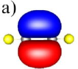
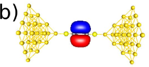
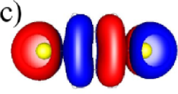
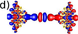
Figure 2: Plots of two orbitals, $\psi$, for di-thiophenyl without electrodes (left) and with $N{E}{=}30$ Au-atoms attached (right). Orbital a) hybridizes only very little with the electrodes and is almost unaffected after coupling, b). By contrast, orbital c) becomes completely delocalized in the metal, see d). Grey (black) colors indicate regions with $\psi$ positive (negative).

Fig. 1 shows, how the six orbitals of the molecule in the gas-phase shift and hybridize with $N_{\mathpzc{E}}$ increasing from $0,1,5,14,30,71$. For illustration, we have also given the Kohn-Sham wavefunctions of two representative states in Fig. 2.

The overall plot clearly shows, that the original orbitals survive the coupling to the electrodes and therefore contribute as resonances to the transport characteristics. The initial evolution at small $N_{\mathpzc{E}}$ is not very smooth, which is because a) attaching the first few Au-atoms cannot be considered a very small perturbation to the molecular system and b) at “magical” numbers of atoms, e.g. $N_{\mathpzc{E}}{=}5$, the electrode configuration is particularly stable. These “stability” islands are interesting in themselves but for our present purpose they deliver parasitic side effects, since they make it more difficult to extrapolate the overall flow. When keeping away from exceptional numbers, e. g. taking $N_{\mathpzc{E}}{=}14,30,71$, the evolution shows the expected smooth behavior.

We have already mentioned, that the smooth evolution of single particle levels can also be perturbed, if a prominent molecular level happens to cross the Fermi energy. This can happen in a situation where the HOMO is relatively close to $E_{\rm F}$. Then small fluctuations of the charge distribution, that occur due to the gradual appearence of “evanescent” modes, i.e. invading electrode states with energies in between the prominent molecular orbitals, can lift the (designated) HOMO above $E_{\rm F}$ at certain electrode configurations.

This is what is happening with Au55 electrodes, as can be seen from Fig. 3. In this case a molecular state (that turns out to be localized predominantly on the S-atoms) peaks above $E_{\rm F}$ and therefore is evacuated, leading to a decrease of the charge accumulated on the molecule by 1.2$e$. The fate of this prominent mode that has been expelled from the region of occupied energy levels is a fast decay with further increasing $N_{\mathpzc{E}}$, because of its relatively strong coupling to the “invaders”, see Fig. 3.

So far we have witnessed the transformation (or in some cases the decay) of the states, that occurs as a consequence of the hybridization of electrode and molecular orbitals. In a sense, this is the analogue of Fermi-liquid theory. The Kondo-effect, which in principle could appear for molecular systems that carry a spin, cannot be understood within this picture. This is because the Abrikosov-Suhl resonance is not a shifted molecular level. Instead, it is a collective phenomenon and generated by a large number of electrode states. Their energies reside inside HOMO-LUMO gap of the “dressed” molecule close to the Fermi-energy. This effect can be seen with DFT in principle, but the current approximations for the exchange correlation functional are too crude in order to capture it. A study with the exact, at present unknown functional should show satellites at $E_{\rm F}$ produced by lead states that merge with one another if the system size becomes large. If sufficiently many of them superimpose, a sharp peak, the Abrikosov-Suhl resonance, grows right within the HOMO-LUMO gap. A further typical characteristics of this collective effect is, that the resonance position is always the Fermi energy, irrespective of shifts in the molecular orbital energies, that might be induced by a gate, for instance.

Figure 3: Plot similar to previous Fig. 1 with $N_{\mathpzc{E}}{=}55$ included. A right shift of the prominent orbitals is caused in the center panel because of additional, “evanescent” modes appearing.

2.2 Extended Molecule and $\Sigma_{e\mathpzc{M}}$

The self energy of the original molecule, $\Sigma_{\mathpzc{M}}$, can contain a wealth of nontrivial information, it is not a quantity easy to calculate. This was the message of the preceeding section. However, the situation greatly simplifies, after the molecule has been redefined. Let us consider an extended molecule, $e\mathpzc{M}$, that comprises in addition to the original molecule also a “contact region”, i. e. a number $N_{\mathpzc{E}}$ of electrode atoms. The Green’s function for an extended system, $G_{e\mathpzc{M}}$, is related to the full Green’s function $G$ via a new self energy

$$G^{-1}(E)=G^{-1}_{e\mathpzc{M}}(E)-\Sigma_{e\mathpzc{M}}(E).$$ (8)

We give two reasons, why it is that $\Sigma_{e\mathpzc{M}}$ is much easier to handle than $\Sigma_{\mathpzc{M}}$.

Imagine the extreme limit, in which far more electrons are sitting on the metal than on the molecule. Then the HOMO of the big system, $\epsilon_{\rm H}$, is given by the Fermi energy of the metal, $E_{\rm F}$, up to a small uncertainty, which is of the order of the HOMO-LUMO gap of $e\mathpzc{M}$, $\delta_{\rm HL}$. In a metal, this gap is inversely proportional to the number of metal electrons in the calculation, $\delta_{\rm HL}\propto 1/N_{e\mathpzc{M}}$, so that the uncertainty of the position of the Fermi energy with respect to $\epsilon_{\rm H,L}$ can be made arbitrarily small. This is a very obvious advantage.

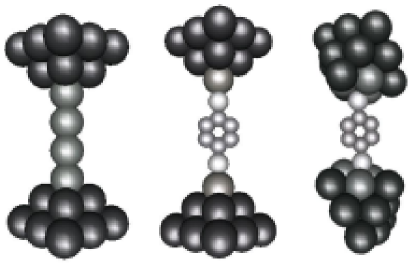
Figure 4: Atomic configurations of molecular junctions attached to pieces of the electrodes. Electrodes are modeled by pyramids, $N_{\mathpzc{E}}{=}14$ Au-atoms each. Dark atoms are surface atoms used in self energy (29). Left: 2 Au-atom wire, $N_{\mathpzc{S}}{=}13$ (Sec. 4.1). Center: di-thiophenyl with (stretched) ${\rm S-Au}_{1}$ coupling; 2 sulphor, six carbon atoms, $N_{\mathpzc{S}}{=}13$ (Sec. 4.2). Right: di-thiophenyl with relaxed ${\rm S-Au}_{3}$ coupling, $N_{\mathpzc{S}}{=}11$ (Sec. 4.2).

More importantly, the flow of the typical level broadening, $\gamma_{\rm H,L}$ (related to $\Sigma_{e\mathpzc{M}}$), that is driven by increasing the number of electrode atoms, $N_{\mathpzc{E}}$, in the contact region, will lead us into a very tractable regime as we shall see now. It is only a fraction $N_{\mathpzc{S}}$ of the $N{E}$ electrode atoms that is actually connected to the rest of the leads, the “outside world”. Assume, that $N_{\mathpzc{E}}$ grows in such a fashion, that the number of these “surface atoms”, $N_{\mathpzc{S}}$, does not change, so we build a quasi-one-dimensional wire. Then, increasing $N_{\mathpzc{E}}$ implies, that the fraction of the wavefunction amplitude of extended orbitals sitting near the surface decays like $N_{\mathpzc{S}}/N_{\mathpzc{E}}$, so that $\gamma_{\rm H,L}$ scales like $\delta_{\rm HL}$. In good metals the ratio of both energies is of the order of the metallic conductance

$$\gamma_{\rm H,L}/\delta_{\rm HL}\sim g\apprge 1.$$ (9)

So, the level broadening of HOMO and LUMO of the extended molecule always exceeds their separation if the electrodes are made from a good metal. This is a situation, exactly opposite to the problematic one, $\gamma_{\rm h,l}/\delta_{\rm hl}\ll 1$, that we have encountered before in the context of (7). Summarizing, for the extended molecule, $e\mathpzc{M}$, the following hierarchy of inequalities holds true (10).

$$\delta_{\rm HL}\leq\gamma_{\rm H,L}\ll\gamma_{\rm h,l}\leq\delta_{\rm hl}.$$ (10)

The separation of energy scales implied by (10) is the prerequisite for the real gain that one makes when one turns to the extended molecule. The point is that the fine structure in the spectrum of $G_{e\mathpzc{M}}$ is on the scale of $\delta_{\rm HL}$. The anti-hermitian constituent of $\Sigma_{e\mathpzc{M}}$, $\gamma_{\rm H,L}$, provides the smearing of this fine structure necessary in order to obtain smooth curves, e.g. for spectral and transmission functions. The details of this smearing have very little impact on the resulting curves, because the interesting structures live on energy scales $\delta_{\rm h,l}$ and $\gamma_{\rm h,l}$, which exceed $\delta_{\rm HL}$ and $\gamma_{\rm H,L}$ by a parametrically large factor.

2.3 $\Sigma_{e\mathpzc{M}}$ and Absorbing Boundary Conditions

There is yet another, perhaps particularly intuitive way to understand the principal difference between $\Sigma_{\mathpzc{M}}$ and $\Sigma_{e\mathpzc{M}}$. It will serve as a motivation for the proposed approximation (5).

Let us assume, we opted for an investigation of transport properties in the time domain, e. g. by propagating wavepackets. Then, we would study the time evolution of a wavepacket, that is localized at $t{=}0$ at some initial position on the molecule. In particular, we can investigate how wavepackets leak out of the molecule into the contacts such that they gradually disappear. When performing such an investigation systematically in the presense of leads, one can in principle collect enough information in order to reconstruct the Fourier transform of the retarded Green’s function, $G(t)$.

There is a condition on the observation time, $T$. In order to have an energy resolution $\gamma_{l,r}$ we need $T\apprge\gamma_{l,r}^{-1}$. This comes for us with trouble, if the contact size maintained in our calculation is not sufficiently large. After some time, the leakage will hit the outside walls of the contact, reflect back off them and finally, after the “dwell” time, $\tau_{D}$, it will rearrive at the molecule; we calculate $G_{e\mathpzc{M}}(t)$ instead of $G(t)$. The energy resolution, that we achieve with such a calculation, can not exceed $h/\tau_{\rm D}$. The best that we can hope for is $\tau_{\rm D}\sim\delta_{\rm HL}^{-1}$ but only in a case, where the contact acts as a fully chaotic cavity. At longer times the signal from the decaying wavepacket will be superimposed by the cavity modes that describe how the wavepacket sloshes back and forth inside the electrodes. We shall demonstrate this effect in Sec. 3 looking at an explicit example.

The salient point we wish to make is, that the minimum dwell time in the cavity should be so long that the wavepacket has enough time to evacuate before the molecule is being refilled again from the backscattered modes:

$$\tau_{D}\gamma{l,r}\gg 1.$$ (11)

There is a very elegant and powerful procedure that eliminates spurious cavity modes so that the condition (11) is always satisfied: one introduces absorbing boundary conditions (abc) in some regions of the cavity. These “surface” regions should swallow incoming signals, i.e. wave packet amplitude, and thus properly mimic escape to infinity. If the wavepackets, bouncing hence and forth inside the cavity, are completely eliminated before the return time $\tau_{\rm D}$ has passed, no trace of the finite cavity/electrode size will be left and $G(t,{\bf x},{\bf x^{\prime}})$ can be reconstructed. This is exactly how adding the self energy $\Sigma_{e\mathpzc{M}}$ works and nothing more than this is implied, if the contacts are sufficiently large. Therefore, we are entirely free to replace the exact boundary conditions $\Sigma_{e\mathpzc{M}}$ by any other ones, provided they absorb sufficiently fast (and do not disturb the immediate vicinity of the molecule-electrode junction).

This is the idea underlying the step proposed in (5). From what has been said above, it should have become clear that this ansatz is actually not just a good approximation, but it will give exact results, if the number of metal atoms $N_{\mathpzc{E}}$ is sufficiently large and the damping function has been chosen well enough. The examples given in Sec. 4 suggest, that a relatively small number of contact atoms $\sim 10-20$ can already give reasonable results.

3 Toy Models

In this section we are going to analyze two toy problems as test cases, namely the conductance of an $L$-site tight binding wire, clean and in the presence of an obstacle, that mimics a molecule.

We will begin with a single channel wire and show, that the technique introduced with (7) delivers the correct answer. This test case is interesting, because a) the numerical results can be compared to analytical formulas and b) it is particularly difficult, in the sense that the dwell time, $\tau_{D}\approx L/2v_{\rm F}$, is (untypically) small ($v_{\rm F}$: Fermi velocity). To illustrate the method further, we also apply it to a wire with four channels and show, that not only the conductance but also more complicated quantities, like the local current density, can be obtained.

3.1 Single Channel Tight Binding Wire

Figure 5: Single channel tight binding wire with triple barrier realized by weak links (indicated by vertical double lines) as used in model calculations.

Models and Analytical Results

The model Hamiltonian of the clean tight binding wire is given by

$$H=-t/2\sum_{i{=}1}^{L}c^{\dagger}_{i}c_{i+1}+c^{\dagger}_{i+1}c_{i}$$ (12)

for spinless, non-interacting electrons. The corresponding dispersion relation reads

$$\epsilon_{k}=-t\cos(ka),$$ (13)

where $a$ denotes the lattice constant, and for the density of states one has

$$\varrho(E)=\frac{1}{\pi t\sqrt{1-(E/t)^{2}}}.$$ (14)

It exhibits the usual van Hove singularities at the edges of the band, which can also be seen in Fig. 6.

In order to calculate the transport coefficient of the $L-$chain defined in (12) we should couple it adiabatically to a left and a right hand side reservoir. This can be done by attaching further half-infinite tight binding chains to the right and the left  of the $L-$chain. The combined system is a perfect 1$d$ crystal. Its Bloch waves travel without any backscattering through the $L-$chain and therefore it is a perfect conductor with transmission unity:

$$T(E){=}1\qquad|E|<t$$ (15)

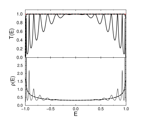
Figure 6: Clean single channel tight binding wire, upper panel: transmission. Analytical result (15) (solid,thin) and numerical result for $L{=}256$ with fully absorbing boundary conditions (dashed; $i{S}{=}32$, $\beta{=}0.3$, $\eta{=}1$). Also shown is numerical result with partially absorbing boundary conditions for $L{=}16$ (solid, wiggly line, $i{S}{=}1$, $\beta{=}\infty$, $\eta{=}1$). Lower panel: density of states corresponding to the transmission curves shown in upper panel.

Next, let us insert an obstacle, e. g. a strong triple barrier (see Fig. 5), into the wire, a situation that still can be understood in all detail. The corresponding Hamiltonian $H_{e\mathpzc{M}}$ is realized with hopping amplitudes occurring in (12) that take the values $t{=}0.05$ at the pairs of sites $(i_{\pm}{=}L/2,i_{\pm}{=}L/2\pm 2)$ and $t{=}1$ everywhere else.

The triple barrier has two eigenstates, a symmetric and an anti-symmetric one, which are energetically nearly degenerate since the center barrier is high. The energy is given approximately by the width of the double well inside the outer barriers, $3a$. It corresponds to a wavenumber $k=\pi/3a$ which in turn implies a resonance energy close to $t/2$. Therefore, the transmission characteristics of the triple barrier should exhibit a superposition of two Lorentzians, one slightly below and one slightly above $E=t/2$. These are the features that can indeed be seen in the analytical result for the conductance (valid in the limit of weak coupling, $V\ll t$)

$$T(E)=\sum_{\alpha{=}\pm}\frac{1}{1+\gamma^{-2}(E-E_{\alpha})^{2}}$$ (16)

where $E_{\pm}{=}\cos(\pi/3{\pm}V\sin(\pi/3)/3)$, $t{=}1$ and $\gamma{=}V^{2}\sin(\pi/3)^{3}/24$. A derivation can be found in appendix 7. Here, we have reproduced for better clarity only an expansion of the exact answer, given in (32), which is valid in the vicinity of the resonances. We also display the exact transmission in Fig. 7, upper panel.

Figure 7: Transmission of a single channel wire with a strong triple barrier (see text). Upper panel: exact analytical result. Center: deviation of numerical results from analytical calculation: $\ln\frac{T(E)}{T_{a}(E)}$ ($L{=}256$, $i{S}{=}32$, $\beta{=}0.3$, $\eta{=}1$, dashed; $L{=}64$, $i{S}{=}16$, $\beta{=}0.3$, $\eta{=}1$, dotted) with absorbing boundary conditions. Lower panel: partially absorbing boundary conditions (dotted, wiggly line: $L{=}16$, $i{S}{=}1$, $\beta{=}\infty$, $\eta{=}1$) (solid, smooth line: $L{=}64$, $i{S}{=}1$, $\beta{=}\infty$, $\eta{=}1$)

Green’s Function Method with Absorbing Boundary Conditions

The transmission of the combined system – wire plus triple barrier – has been given already in (1). In the present case it reads

$$g(E)=\text{Tr}{eM}\ G\Gamma_{\mathpzc{L}}G^{\dagger}\Gamma_{\mathpzc{R}},$$ (17)

where the definition of $G$, (4), implies:

$$G^{-1}=E-H_{e\mathpzc{M}}-\Sigma_{\mathpzc{L}}-\Sigma_{\mathpzc{R}}.$$ (18)

The Hamiltonian $H_{e\mathpzc{M}}$ of the extended molecule is given with Eq. (12) and the trace $\text{Tr}_{e\mathpzc{M}}$ is over the corresponding Hilbert space. The operators $\Gamma_{\mathpzc{L,R}}$ are related to those pieces, $\Sigma_{\mathpzc{L,R}}$, of the self energy, $\Sigma_{e\mathpzc{M}}$, which describe the level broadening due to the coupling to the left ($\mathpzc{L}$) and right ($\mathpzc{R}$) leads:

$$\Gamma_{\mathpzc{L,R}}=i(\Sigma_{\mathpzc{L,R}}-\Sigma_{\mathpzc{L,R}}^{\dagger}).$$ (19)

The precise form that the $\Sigma_{\mathpzc{L,R}}$ take, depends on how we couple the wire to the external leads. In the spirit of section Sec. 2.3, we simply define $\Sigma_{\mathpzc{L,R}}$ as follows:

$$\Sigma_{ij;{\mathpzc{L}}} = i\eta_{i}\delta_{ij};\qquad\eta_{i}{=}\eta/(1+\exp{\beta(i-i{S})})$$ (20)

$$\Sigma_{ij;{\mathpzc{R}}} = i\eta_{i}\delta_{ij};\qquad\eta_{i}{=}\eta/(1{+}\exp{\beta(L{-}i{-}i{S})}).$$ (21)

Three parameters have been introduced: $\eta$ is the atomic leakage rate for all those atoms that are fully coupled to the outside; $i{S}$ describes the number of surface atoms on either side of the molecule; $\beta$ is the adiabaticity parameter, that models a smooth transition into the external wire.

Fig. 6, upper panel, displays the result of this procedure for the transmission of the clean wire. As expected, the exact result (15) is recovered in the case with perfectly absorbing boundary conditions (abc). For comparison, we also show a trace corresponding to incomplete absorption. The cavity modes manifest themselves in the transmission characteristics as relatively sharp resonances. In order to highlight this aspect, the lower panel of Fig. 6 also shows the density of states of the wire.

In Fig. 7 we present the transmission of the single channel wire with a triple barrier implantation. As can be seen from the upper panel, the agreement between the wire with fully abc and the analytical result is perfect. Once more we also display traces that result from a calculation with imperfectly absorbing boundaries. Traces for two different cavity sizes, $L{=}16,64$, are given. Like in the previous case, Fig. 6, the cavity eigenmodes give rise to system size dependencies, which are the spurious resonances in the transmission characteristics. By contrast, no remnant of the system size is left if perfect abc are used, see upper panel traces for $L{=}64,256$.

Let us emphasize, that the good quality of the results Fig. 6 and 7 is not a consequence of fine-tuning parameters. We have ascertained, that the traces corresponding to perfectly abc are stable against variations at least in the parameter range $L{=}64{-}512$, $\eta{=}0.1{-}10$, $\beta{=}0.03{-}0.5$, $i{S}{=}8{-}64$.

In the test cases presented in this subsection, analytical results have been available in order to demonstrate that the choice of parameters associated with the absorbing boundary conditions was appropriate. In more realistic situations analytical results are almost never available. Therefore additional criteria have to be given so as to establish that a certain choice of boundary conditions indeed provides sufficient absorption. The basic rule is, that a good implementation will yield transmission curves that are (largely) independent of the size $N_{e\mathpzc{M}}$ of the cavity, of the choice of surface atoms inside the cavity and of the atomic leakage rate $\eta$. A calculation, that satisfies these requirements, is (usually) quite reliable.

3.2 Local Currents in a Many Channel Tight Binding Wire

As a further application of our method, we calculate the local current density, $j_{\mu}$, in a multi-channel wire. We begin by deriving a general formula relating $j_{\mu}$ to the Green’s functions and self energies, that have been calculated in the preceeding section. Thereafter, we shall illustrate the result by calculating the local current distribution within a double well embedded in a four channel wire.

Lattice Current Density in Terms of Green’s Functions

To start with, we consider the general model Hamiltonian

$$H=\frac{1}{2}\sum_{\nu,\nu^{\prime}}t_{\nu,\nu^{\prime}}\ c^{\dagger}_{\nu}c_{\nu^{\prime}}.$$ (22)

The multi-index $\nu$ comprises the longitudinal, $i_{\nu}$, and transverse, $\ell_{\nu}$, wire coordinates. An expression for the local (longitudinal) current density may be obtained from the time dependent local density:

$$\dot{n}_{\mu}=\frac{i}{\hbar}[H,c^{\dagger}_{\mu}c_{\mu}]=-\frac{i}{2\hbar}\sum_{\nu}t_{\mu\nu}c^{\dagger}_{\mu}c_{\nu}-t^{*}_{\mu\nu}c^{\dagger}_{\nu}c_{\mu}.$$ (23)

The component of the local particle current in the longitudinal direction (right), $j_{\mu}$, is given by the difference of those hopping events that enter site $(i_{\mu},\ell_{\mu})$ from the left and leave there again:

$$j_{\mu}=-\frac{i}{2\hbar}\sum_{i_{\nu}<i_{\mu}}\sum_{\ell_{\nu}}t_{\mu\nu}c^{\dagger}_{\mu}c_{\nu}-t^{*}_{\mu\nu}c^{\dagger}_{\nu}c_{\mu}.$$ (24)

The expectation value of this operator is readily expressed in terms of the Green’s function meir92 , $G^{<}_{\nu\mu}(t,t^{\prime}){=}i\langle c^{\dagger}_{\mu}(t^{\prime})c_{\nu}(t)\rangle$,

$$\langle j_{\mu}\rangle=-\frac{1}{2\hbar}\int\!\frac{dE}{2\pi}\ \sum_{\nu}^{\mathpzc{L}_{\mu}}t_{\mu\nu}\ G^{<}_{\nu\mu}(E)-t^{*}_{\mu\nu}\ G^{<}_{\mu\nu}(E).$$ (25)

In order to simplify the notation, we have introduced a name for sums like the one appearing in (24), which are restricted to the left/right half space: $\sum^{\mathpzc{L,R}}$. Since we only consider non-interacting fermions, $G^{<}_{\nu\mu}$ takes a particularly simple form (e. g. datta95 )

$$G^{<}=iG\left(f_{\mathpzc{L}}\Gamma_{\mathpzc{L}}+f_{\mathpzc{R}}\Gamma_{\mathpzc{R}}\right)G^{\dagger},$$ (26)

which in the limit of small voltages $V$ leads to the following formula for the local charge current distribution $j(i_{\mu})=\sum_{\ell_{\mu}}j_{\mu}$:

$$e\langle j(i_{\mu})\rangle{=}{-}\frac{ie^{2}}{2h}\!V\!\int\!\!dE\ \frac{df}{dE}\ \sum_{\ell_{\mu}}\sum_{\nu}^{\mathpzc{L}_{\mu}}t_{\mu\nu}\left[G\left(\Gamma_{\mathpzc{L}}{-}\Gamma_{\mathpzc{R}}\right)G^{\dagger}\right]_{\nu\mu}.$$ (27)

(When writing this expression, we have assumed for simplicity that $H$ is time reversal invariant, so that $t$ is real and $t,G$ and $\Gamma$ are symmetric matrices. Also, $f_{\mathpzc{L,R}}$ denote the Fermi-Dirac distribution of quasi-particles in the left and right hand side reservoirs.)

Application: Double Dot Inside a Four Channel Wire

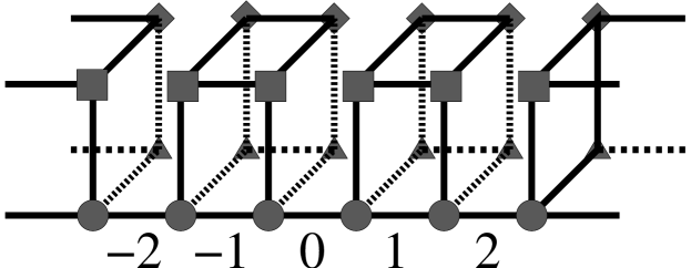
Figure 8: A double dot inside a tight binding wire consisting of four coupled strands (indicated by different symbols).

In order to give an example for the usefulness of (27), we calculate $j_{\mu}$ for a four channel wire with a double well barrier. The example illustrates, that the average current in the wire is a sum of contributions. They can undergo strong spatial fluctuations which are of the order of the mean current and in particular they can be positive or negative (backflow). It is only the sum of all of them which is independent of the longitudinal spatial coordinate.

The clean 4-wire considered here is made up from four strands, which are the 1-wires given in (12). These 1-wires are arranged in a 4-fold cylindrical geometry and in transverse direction only nearest neighbors are being coupled, see Fig. 8. The coupling between all nearest neighbor pairs has been chosen $t{=}2$, except for those 9 pairs, that form the double well. They have $t{=}0$. The position of these “defects” can be given in terms of the longitudinal site index, $i$, and the transverse index $\ell$, that labels the constituting 1-wires in a clockwise fashion: $\ell=0,1,2,3$. We have switched off three couplings at and near the center ($i_{C}{=}L/2$) of the wire, $i_{C},i_{C}\pm 2$, with site indices $\ell{=}1,2,3$. After the definition of the model Hamiltonian, $H_{e\mathpzc{M}}$, we also give the left and right contributions to the self energy $\Sigma_{e\mathpzc{M}}$,

$$\Sigma^{\ell\ell^{\prime}}_{ij;{\rm X}}=\delta_{\ell\ell^{\prime}}\Sigma_{ij;{\rm X}},\qquad{\rm X}={\mathpzc{L,R}}$$ (28)

with a self energy per strand, $\Sigma_{ij;{\rm X}}$, as in (20, 21).

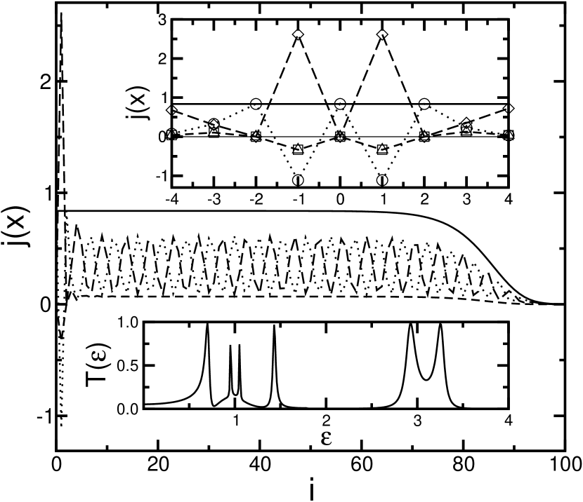
Figure 9: Local current density inside a four channel wire ($L{=}256$, $i{S}{=}32$, $\beta{=}0.1$, $\eta{=}1$) with a double dot (Fig. 8) at $\epsilon{=}0.7$ very close to a resonance of the transmission (see lower inset). Upper inset: behavior near the dots (position $\pm 2,0$). Channels $1,3$ ($\Box,\triangle$, dashed line; same current density) and $2$ ($\diamond$,long dashed) are blocked, channel zero $0$ ($\circ$, dotted line) remains open. Inside the wells, $j_{2}$ overshoots the transmission (solid line) by 300 %, so that local backflow in the other current channels is generated. Main: sum of local currents (solid line) is conserved, i.e. independent of position (except for the surface region, where by adding the self energy leakage has been introduced).

Again, we may employ (18, 19), so that the numerical evaluation of (27) is straightforward ($T{\to}0$). Fig. 9 shows the induced current density per applied voltage near the resonance energy, $\epsilon=0.7$. Before we discuss this result in more detail, we first address the structure of the transmission function which is also displayed in Fig. 9, lower inset. It consists of three pairs of resonances, each pair resembling the symmetric and anti-symmetric eigenstate of the (isolated) double well. The pair of peaks closest to the band edges originates from hybridization of these states with those wire modes, that have a wavenumber matching $\pi/2a$ and an $s$-wave type symmetry in transverse direction. In these two peaks the current density is homogeneously distributed among the four constituting wires. The last sentence is not true for the remaining two pairs of resonances with $p$-wave character, where the current flows mainly in one of the wire pairs, either (0,2) or (1,3). Evidently, the two resonances closest to $\epsilon{=}1$ belong to the second category, since these are much sharper and less well split than all the others.

Now, we can come back to the strong oscillations seen in the local current density of the resonance closest to the band center, main panel of Fig. 9. There, the current flow is mostly in the (0,2) pairs. Since due to the barrier these two channels are not symmetry equivalent, the current densities $j_{i0}$ and $j_{i2}$ can pick up different dependencies on the longitudinal wire coordinate, $i$. In fact, this must be the case since at the barrier position $j_{0}{=}1$ while $j_{2}{=}0$.

The phase locking between the local currents flowing along the (0,2) pair of strands has an interesting effect on the current flow inside each well: in this region, the component $j_{2}$ acquires a value three times exceeding the average current flow. This value is compensated by a backflow in the other channels, so that a current vortex develops.

4 Test Cases from Quantum Chemistry Calculations

The purpose served by the tight binding calculations of the previous chapter was to demonstrate the principle. High precision in the calculations performed there was relatively easy to achieve, because the parameter space representing a perfect separation of energy (or time) scales was well accessible to numerical methods.

In the case of quantum chemistry calculations that are feasible at present, the accessible system sizes often are not large enough in order to achieve such a clear scale separation. What we demonstrate in this section is, that our method operates reasonably well, also in a practical situation, where scale separation is not perfect.

To this end, we shall consider two extreme cases, a short gold chain with a conductance $g\sim 1$ and a molecule, di-thiophenyl with $g\ll 1$. Both objects are coupled to the tip of two tetragonal bipyramids of 14 Au-atoms each, that represent the extension modelling a piece of the electrodes, see Fig. 4. We define an effective single particle Hamiltonian, $H_{e\mathpzc{M}}$, for these systems in the way explained in Sec. 2.1.

The proposed construction mechanism has been formulated in coordinate (real) space. Therefore it matches particularly well with quantum chemistry calculations, that are using the local atomic basis sets $|X,\ell\rangle\equiv|b\rangle$ also introduced in Sec. 2.1. Adopting (5) to the present case, we introduce the following self energy:

$$\Sigma_{\rm X}=i\eta\sum_{b,b^{\prime}}^{\mathpzc{S}_{\rm X}}|b\rangle\ [S^{-2}]_{bb^{\prime}}\ \langle b^{\prime}|,\qquad{\rm X}={\mathpzc{L,R}}.$$ (29)

The overlap matrix, $S_{bb^{\prime}}=\langle b|b^{\prime}\rangle$, that appears in this expression takes care of the fact, that basis states belonging to different atomic sites will not be orthogonal in general. $\Sigma_{\mathpzc{L,R}}$ is local, i.e. diagonal in the atomic basis set $|b\rangle$, in full analogy to (20, 21). Again the important input is in the strength and spatial modulation of the leakage function. In the present case, we choose it to be a constant, $\eta$, for a subset $\mathpzc{S}_{\mathpzc{L,R}}$ of “surface atoms” and zero for all the others. In our calculations we take these sets to be the two layers of the pyramid ($3\times 3$ and $2\times 2$) that are farthest from the molecule, see Fig. 4.

Figure 10: Upper panel: Transmission of a two atom Au-chain linked to the tip of two tetragonal pyramids of 14 Au-atoms each. Self energy (29) has been used. Three traces with different $\eta$ are shown: 2.72 eV (dashed), 0.81 eV (solid), 0.27 eV (dotted). The $\Box$-symbol indicate the result with the canonical coupling and much larger pyramids with 55 atoms evers03prb . Lower panel: density of states calculated with the Green’s functions used in the upper plot. Also the density of states for bulk gold is shown (symbol $\times$).

4.1 Transmission of Au-Chain

We begin our analysis with the two atom Au-chain. The transmission of such chains has been studied by various groups before brandbyge02 ; palacios02 . It is well known that reproducing the correct transmission curve is a sensitive test on the quality of the damping $\Sigma_{e\mathpzc{M}}$ of the model. In Fig. 10, upper panel, we depict the transmission as obtained from the model (29). For comparison, also plotted is a result obtained from a much larger system with a self energy calculated directly from (3) (where $G{S}$ has been replaced by the bulk Green’s function $G{B}$) evers03prb . Agreement for the two larger values of the coupling amongst each other and also with the original curve is established reasonably well with deviations typically less than 10 %.

As was to be expected, the window of $\eta$-values in which one finds good quantitative agreement between the various curves is relatively small. This is simply because of the very small cavity size. In fact, the “molecule” defined by the two Au-atoms in line, see Fig. 4, are separated from the effective surface regions $\mathpzc{S}_{\mathrm{L,R}}$ by only one gold atom.

In the surface regions, the model self energy somewhat modifies the local material parameters, like the density of states (DoS). This can be seen in Fig. 10, lower panel. The total DoS is strongly dominated by surface atoms. It has a dependency on $\eta$ that is much stronger than the one of the transmission Fig. 10, upper panel. Note, that this modification will have a substantial impact, if one were to set up a self consistent calculation with a local density obtained from the dressed Green’s function (4). The present setup is not (and in fact does not need to be) self consistent in this sense, and therefore the modification of the surface spectral function will be without consequences for the transport calculations proposed here.

We comment on the absence of a adiabaticity parameter $\beta$ in the definition of the self energy (29). The pyramids simulating the electrodes act as resonating cavities in the same way that the single channel tight binding wire does, c.f. Sec. 3.1. However, the tight binding wire was special, in the sense that the number of surface atoms coupling to the infinite tight binding chain was only two, independent of the volume of the wire, $L$. For this reason the resonator modes had to be eliminated by introducing the adiabaticity parameter $\beta$. In higher dimensions, the ratio of contact surface to volume is much more favorable. Therefore the surface damping of the resonator modes is much stronger – no real need to introduce a $\beta$-parameter here.

4.2 Transmission of Di-Thiophenyl

Finally, we apply our construction for the self energy to the paradigm of computational molecular electronics, the di-thiophenyl system. Again, the electrodes are modelled by the same pair of 14-Au pyramids, that we have used before for the 2-Au-chain. Accordingly, the construction of the model Hamiltonian and, in particular, the self energy are just as in the previous section.

We will investigate two slightly different situations, where the sulphur atom, that ties the benzene to the Au-contact surface, once connects to a single Au-atom and once to three of them.

${\rm S-Au}_{1}$ Coupling

Figure 11: Upper panel: transmission of di-thiophenyl with a ${\rm S-Au}_{1}$ coupling (see Fig. 4). for different damping parameters $\eta$: 0.27 eV (dotted), 2.7 eV (solid) and 27.2 eV (dashed). Also shown 30-Au pyramids with conventional coupling (29). Lower panel: probability density $P(\epsilon)$ for eigenvalues (proportional to the DoS). Three traces correspond to the transmission lines of upper panel. Symbols $\times$ indicate $P(\epsilon)$ of bulk gold.

The atomistic setup, that we consider in this subsection, is presented in Fig. 4. The S-atom acts as the barrier that disconnects the conjugated $\pi$-system of the phenyl ring from the Au-atom forming the tip of the pyramid. This atom provides the separation for the junction from the contact region which is necessary in order to find results for the transmission independent of the choice of $\eta$ within a large parameter window.

Indeed, our expectations are well confirmed by the numerical data. Fig. 11, upper channel, shows transmission lines for $\eta$ varying over two orders of magnitude. All traces faithfully reproduce the salient resonance structures in the vicinity of 1 eV about the Fermi energy, $E_{\rm F}=-5.05$ eV. In this regime, the transmission is almost unaffected by the change in $\eta$ even though the average DoS changes by a factor of three, see Fig. 11, lower panel. Eventually, there is an impact of $\eta$ in the tails of the resonances, where the transmission is small and the DoS changes with $\eta$ by an order of magnitude. This regime can be better controlled by creating an additional spacer layer of Au-atoms between the contact atoms and the junction.

We believe, that the construction principle (29) is well suited to model the line broadening of resonances. There is, however, no prediction as for the line shift, of course. Line shifts occur, e. g. when charge reorganization takes place, involving charge flow from one subsystem to another. Such processes can be reliably modelled only by increasing the number of electrode atoms in the calculation and monitoring the results.

${\rm S-Au}_{3}$ Coupling

In this paragraph, we investigate a situation in which the S-atoms couple to three Au-atoms rather than just one. There are two motivations for doing so. First, a two or three site configuration of the sulphur is energetically more favorable than the single site coordination used in Sec. 4.2 and thus more likely to be relevant for the understanding of experiments evers03prb . Second, we would like to present a simple example for a situation, where the dwell time in the cavity is not sufficiently long so that the parameter window has closed, in which the transmission traces are independent of the damping $\eta$.

In general, one avoids coupling the S-atoms directly to the surface layers, $\mathpzc{S}_{\rm L,R}$, because the change in the local DoS near the contact may feed back into the transmission. Therefore, for the ${\rm S-Au}_{3}$-coupling (Fig. 4) we include all Au-atoms into $\mathpzc{S}_{L,R}$ except for those three Au-atoms, that bind to $\mathrm{S}$. After this minor modification, calculations proceed in the same way as before.

Figure 12: Transmission of di-thiophenyl with a ${\rm S-Au}_{3}$ coupling (see Fig. 4). Thin traces: 14-Au pyramids with $\eta$ 0.81 eV (dotted), 2.76 eV (solid) and 8.1 eV (dashed). Fat traces: 55-Au pyramids with $\eta$ 2.7 eV (dot-dashed) and conventional coupling (29) (solid).

The resulting transmission is displayed in Fig. 12. For the 14-Au pyramids traces for three different damping values $\eta$ are shown. They vary appreciably one from another and the correct result is recovered only in relatively rough terms. The limited quality of the model coupling in the present case was to be expected. Since the number of surface atoms that couples to the ${\rm S-Au}_{3}$ unit (eight) is much bigger than it was with the ${\rm S-Au}_{1}$ coupling (four), also the dwell time is drastically reduced, too much for our simple model (5) to work with high precision.

The situation is much more favorable if larger cavities are used. Fig. 12 also shows the result for a 55-Au cluster which is in good agreement with the conventional calculation.

5 Discussion and Outlook

The method relying on absorbing boundary conditions (abc), that we have outlined in the preceeding sections, has an important advantage over the more orthodox way of calculating an essentially exact self energy (3): it is much easier to handle. If the abc-calculation meets the requirements listed in Sec. (2.1), then both methods are expected to yield identical results for the Green’s functions.

We have demonstrated how the abc-approach can be combined with standard quantum chemistry calculations for extended molecules, $e\mathpzc{M}$. Because it is not necessary any more to calculate self energies, $\Sigma_{e\mathpzc{M}}$, transport calculations based on the Landauer-Büttiker theory are greatly simplified.

The computational effort is dominated by the quantum chemistry calculation for $e\mathpzc{M}$. Since the number of electrode atoms, $N_{\mathpzc{E}}$, that needs to be included in the calculation, is similar for both methods, one expects that also the computational effort is roughly the same.

The number $N_{\mathpzc{E}}$ is too large in order to allow highly correlated, essentially exact methods to be used for calculating $G_{e\mathpzc{M}}$. However, calculations based on density functional theory can be done very efficiently for these system sizes and also Hartree-Fock calculations are within reach. The last point is of particular interest, because this is a prerequisite to test functionals against each other (BP89, B3Lyp, LHF, etc.), that have a very different degree of self interactions.

These tests are important for the recent debate on the origin of the discrepancy between theoretical and experimental results on the conductance observed for several organic molecules reimers03 ; evers03prb ; kurth:035308 ; sai05 ; burke05a . The conductance of monatomic chains can be investigated very well with the combination of methods, density functional theory (DFT) and Landauer-Büttiker formula, that have been employed in Sec. 4 agrait03 . By contrast, theoretical expectation for the transmission of organic molecules tend to deviate by one or more orders of magnitude from the experimental findings evers03prb .

Apart from experimental difficulties also approximations, that are implicit to the DFT based transport formalism, could very well be responsible for this discrepancy. This is, roughly speaking, because the Green’s functions, that derive from the (ground state) Kohn-Sham-formalism do not necessarily provide a good description of the system dynamics. This description can indeed be acceptable, if electron density is relatively smooth and the system is at least close to metallic, like it is in single atom metal chains. Under these conditions, single particle wavefunctions, which are essentially plane wave states, give a good representation of the spatial properties of the true Green’s function. Then, it is mostly the (local) spectral properties (i.e. the band structure of the atomic wire) that determine the transport characteristics and those can be given quite accurately by present days DFT calculations.

However, organic molecules are a different case, because at least in the vicinity of the contact region, the electron density is far from homogenous. In these regions, the spatial structure of the KS-Green’s function will in general not be a faithful representation of reality, certainly not within local or semi-local approximations of the exchange correlation functional. Since these very regions form exactly the bottleneck for the transport current, theoretical calculations employing such functionals cannot necessarily be expected to be very precise. One can hope, that the useage of non-local functionals will improve upon this situation. Which of the various non-local terms, that exist in the exact (quasi-static non-equilibrium) functional, is the most important one and how to implement it in practical transport calculations, these are at present two of the most thrilling issues in the field of molecular electronics.

6 Acknowledgments

The authors thank K. Busch for drawing their attention to current applications of absorbing boundary conditions in the field of quantum optics. Also, they are indebted to F. Weigend for his help in using the program package TURBOMOLE and numerous instructive discussions. Finally, they express their gratitude to P. Wölfle for helpful comments on the manuscript and in particular for his continuous support of this work. Support has also been received from the Center for Functional Nanostructures at U Karlsruhe and is gratefully acknowledged.

7 A Triple Barrier in a Tight Binding Wire

A one dimensional tight binding chain with only nearest neighbor hopping and three barriers is considered.

The Hamiltonian of this problem is:

$$H_{i,j}=t_{i}\left(\delta_{i,j+1}+\delta_{i+1,j}\right)$$ (30)

with hopping amplitudes $t_{i}$ given by

$t_{M}$	=	$V_{L}$	left barrier
$t_{N}$	=	$V_{C}$	center barrier
$t_{O}$	=	$V_{R}$	right barrier
$t_{i}$	=	$1$	everywhere else

and barriers located at positions $M$, $N$, $O$. The scattering states in the four different sections of the wire can be written as

$\Psi_{j}$	=	$e^{ikj}+re^{-ikj}$	left lead
$\Psi_{j}$	=	$ae^{ikj}+be^{-ikj}$	left to center barrier
$\Psi_{j}$	=	$ce^{ikj}+de^{-ikj}$	center to right barrier
$\Psi_{j}$	=	$te^{ikj}$	right lead

with energy $E(k)=-2\cos k$ (length scales are measured with respect to $a$).

Let us now write down the consequences of the Schrödinger equation left and right of each barrier:

$$E\Psi_{M} = \Psi_{M-1}+V_{L}\Psi_{M+1}$$

$$E(e^{Mik}+re^{-Mik}) = e^{(M-1)ik}+re^{(1-m)ik}+V_{L}(ae^{(M+1)ik}+be^{-(M+1)ik})$$

$$E\Psi_{M+1} = V_{L}\Psi_{M}+\Psi_{M+2}$$

$$E(ae^{(M+1)ik}+be^{-(M+1)ik}) = V_{L}(e^{Mik}+re^{-Mik})+ae^{(M+2)ik}+be^{-(m+2)ik}$$

$$E\Psi_{N} = \Psi_{N-1}+V_{C}\Psi_{N+1}$$

$$E(ae^{Nik}+be^{-Nik}) = ae^{(N-1)ik}+be^{(1-N)ik}+V_{C}(ce^{(N+1)ik}+de^{-(N+1)ik})$$

$$E\Psi_{N+1} = V_{C}\Psi_{N}+\Psi_{N+2}$$

$$E(ce^{(N+1)ik}+de^{-(N+1)ik}) = V_{C}(ae^{Nik}+be^{-Nik})+ce^{(N+2)ik}+de^{-(N+2)ik}$$

$$E\Psi_{O} = \Psi_{O-1}+V_{R}\Psi_{O+1}$$

$$E(ce^{Oik}+de^{-Oik}) = ce^{(O-1)ik}+de^{(1-O)ik}+V_{R}te^{(O+1)ik}$$

$$E\Psi_{O+1} = V_{R}\Psi_{O}+\Psi_{O+2}$$

$$Ete^{(O+1)ik} = V_{R}(ce^{Oik}+de^{-Oik})+te^{(O+2)ik}$$

or in matrix notation:

$$\begin{pmatrix}e^{(M+1)ik}&e^{-(M+1)ik}\\ V_{L}e^{Mik}&V_{L}e^{-Mik}\end{pmatrix}\begin{pmatrix}1\\ r\end{pmatrix} = \begin{pmatrix}V_{L}e^{(M+1)ik}&V_{L}e^{-(M+1)ik}\\ e^{Mik}&e^{-Mik}\end{pmatrix}\begin{pmatrix}a\\ b\end{pmatrix}$$

$$\begin{pmatrix}e^{(N+1)ik}&e^{-(N+1)ik}\\ V_{C}e^{Nik}&V_{C}e^{-Nik}\end{pmatrix}\begin{pmatrix}a\\ b\end{pmatrix} = \begin{pmatrix}V_{C}e^{(N+1)ik}&V_{C}e^{-(N+1)ik}\\ e^{Nik}&e^{-Nik}\end{pmatrix}\begin{pmatrix}c\\ d\end{pmatrix}$$

$$\begin{pmatrix}e^{(O+1)ik}&e^{-(O+1)ik}\\ V_{R}e^{Oik}&V_{R}e^{-Oik}\end{pmatrix}\begin{pmatrix}c\\ d\end{pmatrix} = te^{(O+1)ik}\begin{pmatrix}V_{R}\\ E-e^{ik}\end{pmatrix}.$$

Since, our interest is in the transmission, $T=|t|^{2}$, we only extract an equation for the transmission coefficient, $t$:

$$\Big{[}({V_{L}}^{2}e^{ik}-e^{-ik})({V_{C}}^{2}e^{ik}-e^{-ik})$$ (31)

$$-({V_{L}}^{2}e^{-(2M+1)ik}-e^{-(2M+1)ik})({V_{C}}^{2}e^{(2N+1)ik}-e^{(2N+1)ik})\Big{]}({V_{R}}^{2}e^{ik}-e^{-ik})$$

$$- \Big{[}({V_{L}}^{2}e^{ik}-e^{-ik})({V_{C}}^{2}e^{-(2N+1)ik}-e^{-(2N+1)ik})$$

$$-({V_{L}}^{2}e^{-(2M+1)ik}-e^{-(2M+1)ik})({V_{C}}^{2}e^{-ik}-e^{ik})\Big{]}({V_{R}}^{2}e^{(2O+1)ik}-e^{(2O+1)ik})$$

$$= \frac{8}{t}V_{L}V_{C}V_{R}\sin^{3}k.$$

After specializing to the case of a strong, symmetric barrier, where $V_{L}{=}V_{C}{=}V_{R}$ ${=}V\ll 1$ and $M{=}0$, $N{=}2$, $O{=}4$, we conclude

$$T(k)=\left(2V^{3}\frac{\sin^{3}(ka)}{|\sin^{2}(3ka)-V^{2}\sin^{2}(2ka)+2V^{2}e^{ika}\sin(3ka)\sin(2ka)+\mathpzc{O}(V^{4})|}\right)^{2}$$ (32)

which is also displayed in Fig. 7, upper panel, in the body of the paper, where also a brief discussion of this result may be found.

References

- (1) K. Likharev, A. Mayr, I. Mickra, Ö. Türel: Crossnets: High-peformance neuromorphic architectures for cmol circuits, Ann. N. Y. Acad. Sci. 1006, 146–163 (2003)
- (2) J.R. Reimers, Z.-L. Cai, A. Bilic̀, N.S. Hush: The appropriateness of density-functional theory for the calculation of molecular electronics properites, Ann. N.Y. Acad. Sci. 1006, 235–251 (2003)
- (3) F. Evers, F. Weigend, M. Koentopp: Conductance of molecular wires and transport calculations based on density-functional theory, Phys. Rev. B 69, 235411 (2004)
- (4) S. Kurth, G. Stefanucci, C.-O. Almbladh, A. Rubio, E.K.U. Gross: Time-dependent quantum transport: A practical scheme using density functional theory, Phys. Rev. B 72(3), 035308 (2005)
- (5) N. Sai, M. Zwolak, G. Vignale, M. Di Ventra: Dynamical corrections to the dft-lda electron conductance in nanoscale systems, Phys. Rev. Lett. 94, 186810 (2005)
- (6) K. Burke, M. Koentopp, F. Evers: Zero-bias molecular electronics: Exchange-correlation corrections to landauer’s formula, cond-mat/0502385 (2005)
- (7) Homer. Odyssee, 12. Gesang, Vers 201-259
- (8) D. Bohr, P. Schmitteckert, P. Wölfle: DMRG evaluation of the Kubo formula – conductance of strongly interacting quantum systems, Europhys. Lett. to appear (2005)
- (9) R. Landauer: IBM J. Res. Dev. 1, 233 (1957)
- (10) M. Büttiker, Y. Imry, R. Landauer, S. Pinhas: Generalized many–channel conductance formula with application to small rings, Phys. Rev. B 31(10), 6207 (1985)
- (11) Y. Xue, S. Datta, M.A. Ratner: First-principles based matrix-green’s function approach to molecular electronic devices: General formulation, J. Chem. Phys. 115, 4292 (2001)
- (12) M. Brandbyge, J.-L. Mozos, P. Ordejon, J. Taylor, K. Stokbro: Density-functional method for nonequilibrium electron transport, Phys. Rev. B 65, 165401 (2002)
- (13) Y. Meir, N.S. Wingreen: Landauer formula for the current through an interacting electron region Phys. Rev. Lett. 68(16), 2512 (1992)
- (14) D.S. Fisher, P.A. Lee: Relation between conductivity and transmission matrix, Phys. Rev. B 23, 6851 (1981)
- (15) H.U. Baranger, A.D. Stone: Electrical linear-response theory in an arbitrary magnetic field: A new fermi-surface formation, Phys. Rev. B 40, 8169–8193 (1989)
- (16) R. Ahlrichs, M. Bär, M. Häser, H. Horn, C. Kölmel: Electronic structure calculations on workstation computers: The program system turbomole, Chem. Phys. Lett. 162, 165 (1989)
- (17) K. Eichkorn, O. Treutler, H. Oehm, M. Haeser, R. Ahlrichs: Auxiliary basis sets to approximate coulomb potentials, Chem. Phys. Lett. 242, 652 (1995)
- (18) K. Eichkorn, F. Weigend, O. Treutler, R. Ahlrichs: Auxiliary basis sets for main row atoms and transition metals and their use to approximate coulomb potentials, Theor. Chem. Acc. 97, 119 (1997)
- (19) J. Park, A.N. Pasupathy, J.I. Goldsmith, C. Chang, Y. Yaish, J.R. Petta, M. Rinkoski, J.P. Sethna, H.D. Abruña, P.L. McEuen, D.C. Ralph: Coulomb blockade and the kondo effect in single atom transistors, Nature 417, 722 (2002)
- (20) W. Liang, M.P. Shores, M. Bockrath, J.R. Long, H. Park: Kondo resonance in a single-molecule transistor, Nature 417, 725 (2002)
- (21) H.B. Heersche, Z. De Groot, J.A. Folk, L.P. Kouwenhoven, H.S.J. van der Zant: The kondo effect in the presence of magnetic impurities, cond-mat/0508395v1 (2005)
- (22) A.A. Abrikosov, L.P. Gorkov, I.E. Dzyaloshinski: Methods of quantum field theory in statistical physics (Dover 1963)
- (23) G.D. Mahan: Many Particle Physics, Kluwer Academic / Plenum Publishers, 3rd edition (2000)
- (24) W. Brenig: Statistical theory of heat: Nonequilibrium Phenomena, volume II, Springer Verlag (1989)
- (25) U. Schollwöck: The density-matrix renormalization group, Rev. Mod. Phys. 77, 259–315 (2005)
- (26) J.P. Perdew: Density-functional approximation for the correlation energy of the inhomogeneous electron gas, Phys. Rev. B 33, 8822 (1986)
- (27) A.D. Becke: Density-functional exchange-energy approximation with correct asymptotic behavior, Phys. Rev. A 38, 3098 (1988)
- (28) A. Schäfer, C. Huber, R. Ahlrichs: Fully optimized contracted gaussian basis sets of triple zeta valence quality for atoms li-kr, J. Chem. Phys. 100(8), 5829 (1994)
- (29) S. Datta: Electronic Transport in Mesoscopic Systems, Cambridge University Press (1995)
- (30) J.J. Palacios, A.J. P’erez-Jim’enez, E. Louis, E. SanFabi’an, J.A. Verg’es: First-principles approach to electrical transport in atomic-scale nanostructures, Phys. Rev. B 66, 035322 (2002)
- (31) N. Agrait, A.L. Yeyati, J.M. van Ruitenbeek: Quantum properties of atomic-sized conductors, Phys. Rep. 377, 81–279 (2003)