COMPRESSIBILITY EFFECTS ON THE LIGHT SCATTERED BY A NON-EQUILIBRIUM SUSPENSION IN A NEMATIC SOLVENT

Abstract

We investigate the effects produced on the light scattering spectrum by the anisotropic diffusion of impurities (dye) in a compressible nematic solvent. This spectrum is calculated by using a fluctuating hydrodynamic description when the system is in both, a fully thermodynamic equilibrium state and in a non-equilibrium steady state ($NESS$) induced by a dye-concentration gradient. In the former state, the isotropic pre-transitional as well as the nematic phase of the solvent are considered. We find that the equilibrium spectrum is symmetric (Lorentzian) with respect to the frequency shifts, but anisotropic through its explicit dependence on the ratio of the parallel and normal diffusion coefficients of the dye. The values of these coefficients were taken from experimental measurements of diffusion of methylred and nitrozo di-methyl aniline in a $MBBA$ solvent. We find that the compressibility of the solvent increases the maximum and the width at half height of the Rayleigh peak, with respect to the incompressible case suspension1 . This increase varies between $12\%$ and $25\%$, respectively, when the impurities concentrations is the range of $1\%$ - $5\%$. The $NESS$ induces a coupling between the concentration fluctuations of the dye and the hydrodynamic fluctuations of the solvent. In this case the compressibility effects may increase the maximum and the width of the central peak up to $25\%$, for values of the concentration gradient four orders of magnitude smaller than those considered in the incompressible case. This result indicates that compressibility and mode coupling effects may be significant and that they might be detected experimentally. On the other hand, for the nonequilibrium Brillouin part of the spectrum we find that the intensities of the sound propagation modes are unequal and one of the peaks shrinks in the same amount as the other increases. This asymmetry increases linearly with the magnitude of the solute concentration gradient. The maximum difference between the nonequilibrium and equilibrium contributions to the Brillouin spectrum for various values of the external gradient is also estimated. However, in all cases we find that the amplitude of the Brillouin peaks is several orders of magnitude smaller than the central peak. Therefore, although nonequilibrium effects do produce an asymmetry, our theoretical analysis indicates that these effects are too small to be observed experimentally.

I Introduction

In a previous paper hereafter referred to as $I$ suspension1 , we have analyzed the effects produced by the anisotropic diffusion of impurities in an incompressible nematic solvent. By using a fluctuating hydrodynamic approach we calculated the central Rayleigh peak of the spectrum when the solvent is in both, a fully thermodynamic equilibrium state and in a non-equilibrium steady state $(NESS)$ induced by a dye-concentration gradient. The nonequilibrium states considered in $I$ were close to equilibrium and the driving concentration gradient was taken into account through a local version of the fluctuation-dissipation theorem for the stochastic current of the impurities. In the present work we extend the analysis of $I$ in two aspects. First, instead of introducing spatial inhomogeneities in the fluctuation-dissipation theorem, we consider mode coupling terms relating the concentration fluctuations of the solute and the orientation and velocity fluctuations of the solvent. Secondly, apart from the central peak, in the present work we also calculate the Brillouin part of the dynamic structure factor of the impurities and analyze the mode coupling contribution to the full spectrum of the suspension. For this purpose the compressibility of the solvent is considered explicitly in its equations of motion.

We find that in equilibrium the compressibility of the solvent increases the maximum and the width at half height of the Rayleigh peak, with respect to the incompressible case, by amounts that vary between $12\%$ and $25\%$, respectively, as a function of the impurities concentrations in the range of $1\%$ - $5\%$. In the $NESS$ induced by the concentration gradient, these features of the central peak may increase up to $25\%$, even for values of the concentration gradient which are four orders of magnitude smaller than those considered in $I$. This result indicates that compressibility and mode coupling effects may be significant and that they might be detectable experimentally.

On the other hand, for the Brillouin part of the spectrum in the $NESS$ we find that the intensities of the sound propagation modes are unequal and one of the peaks shrinks in the same amount as the other increases, a behavior that is also predicted and observed for a simple fluid beysens , sengers , law1 . We find that this asymmetry increases linearly with the magnitude of the solute concentration gradient. The maximum difference between the nonequilibrium and equilibrium contributions to the Brillouin spectrum for different values of the external gradient is also estimated. However, in all cases we find that the amplitude of the Brillouin peaks is several orders of magnitude smaller than that of the central peak. Therefore, although nonequilibrium effects are present in the above mentioned asymmetry, our theoretical analysis indicates that these effects are too small and difficult to observe experimentally.

II Model and Basic Equations

As in I, we consider a dilute suspension of noninteracting impurities diffusing through a thermotropic nematic liquid crystal solvent, as depicted in Fig. 1. If the suspension is sufficiently diluted, the dynamics of the impurities does not disturb appreciably the state of the nematic and it may be considered to be in an equilibrium state defined by a temperature $T_{o}$, a pressure $p_{o}$, a vanishing velocity field $\overrightarrow{v}^{o}=0$ and a uniform director’s orientation $\hat{n}^{o}=\left(0,0,1\right)$, corresponding to the homeotropic configuration shown in Fig. 1. X

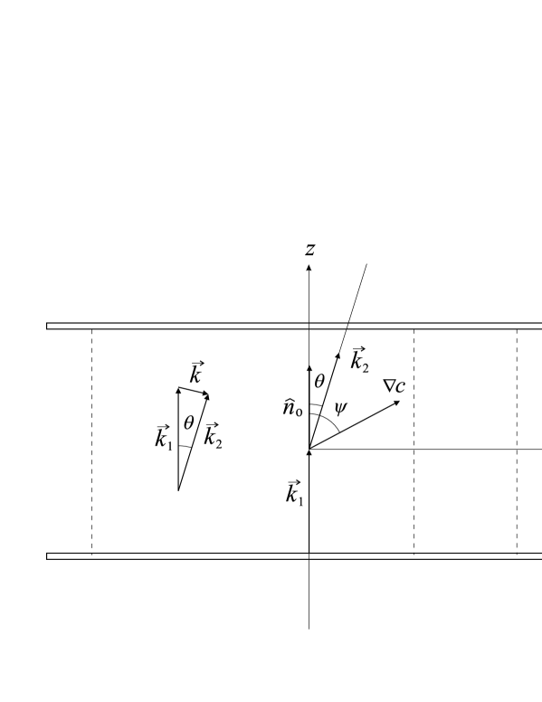
Figure 1: Schematic representation of a plane homeotropic cell with a constant thermal gradient along $z$ direction. The inset shows the scattering geometry.The scattering angle is $\theta$.

We shall only consider nonequilibrium states corresponding to a stationary concentration field of impurities defined by

$$c^{s}\left(\overrightarrow{r}\right)=c_{o}+\overrightarrow{r}\cdot\overrightarrow{a},$$ (1)

where $c_{o}$ is the mean concentration of impurities and $\overrightarrow{a}\equiv\nabla c$ is the uniform concentration gradient in the $y-z$ plane and whose direction is specified by $\psi$. For future use it will be convenient to recast (1) in the more convenient form

$$c^{s}\left(\overrightarrow{r}\right)=c_{o}+a\lim_{q\longrightarrow 0}\frac{\sin\left(\overrightarrow{q}\cdot\overrightarrow{r}\right)}{q},$$ (2)

where $a\equiv\left|\overrightarrow{a}\right|$, $\overrightarrow{q}$ $\equiv\frac{1}{a}\nabla c$ is an auxiliary vector of variable magnitude and parallel to $\overrightarrow{a}$.

If no chemical reactions occur between the impurities, their total number is conserved and their local concentration density, $c\left(\overrightarrow{r},t\right)$, obeys the continuity equation

$$\frac{\partial c}{\partial t}+\nabla_{i}J_{i}=0,$$ (3)

where $J_{i}\left(\overrightarrow{r},t\right)$ is the flux of the diffusing particles, which for an uniaxial nematic is of the form

$$J_{i}\left(\overrightarrow{r},t\right)=-D_{ij}\left(\overrightarrow{r},t\right)\nabla_{j}c\left(\overrightarrow{r},t\right)+c\left(\overrightarrow{r},t\right)v_{i}\left(\overrightarrow{r},t\right).$$ (4)

The first term on the right hand side is the usual Fick’s law contribution where $D_{ij}\left(\overrightarrow{r},t\right)$ is the diffusion tensor of the suspended impurities; the second term represents the convective diffusion of the impurities, where $v_{i}\left(\overrightarrow{r},t\right)$ denotes the velocity field of the solvent. For an uniaxial nematic $D_{ij}$ has the standard form

$$D_{ij}\left(\overrightarrow{r},t\right)=D_{\bot}\delta_{ij}+\left(D_{\parallel}-D_{\bot}\right)n_{i}\left(\overrightarrow{r},t\right)n_{j}\left(\overrightarrow{r},t\right),$$ (5)

where $D_{\parallel}$ is the diffusion coefficient parallel to the director $\widehat{n}\left(\overrightarrow{r},t\right)$ and $D_{\perp}$ is the corresponding coefficient in the perpendicular direction. $D_{a}\equiv D_{\|}-D_{\bot}$ is the corresponding diffusion anisotropy. Usually, the diffusion of small particles dissolved in a nematic solvent is such that the diffusion parallel to the director is faster than perpendicular to it; as a consequence, the ratio $D_{\|}/D_{\bot}$ seems to be independent of the actual shape of the diffusing molecules rondelez , janig , franklin . Using Eq. (5), the diffusion equation for $c(\overrightarrow{r},t)$ turns out to be

$$\frac{\partial}{\partial t}c\left(\overrightarrow{r},t\right) = D_{\bot}\nabla^{2}c+D_{a}n_{i}n_{j}\nabla_{i}\nabla_{j}c$$ (6)

$$+D_{a}\left(n_{i}\nabla_{i}n_{j}+n_{j}\nabla_{i}n_{i}\right)\nabla_{j}c$$

$$-v_{i}\nabla_{i}c+c\nabla_{i}v_{i}.$$

Note that the compressibility of the solvent is taken into account by the term $\nabla_{i}v_{i}\neq 0$, which was absent in $I$.

If a fluctuating mass diffusion current, $J_{i}^{F}\left(\overrightarrow{r},t\right)$, is introduced into this equation, the concentration fluctuations $\delta c(\overrightarrow{r},t)\equiv c(\overrightarrow{r},t)-c^{s}\left(\overrightarrow{r}\right)$, obey the linearized equation

$$\frac{\partial}{\partial t}\delta c = \left(D_{\bot}\nabla_{\bot}^{2}+D_{\|}\nabla_{z}^{2}\right)\delta c+a_{i}\delta v_{i}-c^{s}\nabla_{i}\delta v_{i}$$ (7)

$$+D_{a}\left(a_{i}\nabla_{z}\delta n_{i}+a_{z}\nabla_{i}\delta n_{i}\right)-\nabla_{i}J_{i}^{F}.$$

$J_{i}^{F}\left(\overrightarrow{r},t\right)$ is a Markovian, Gaussian, stochastic processes with zero mean $\left\langle J_{i}^{F}\left(\overrightarrow{r},t\right)\right\rangle=0$ and whose correlation is assumed to obey a local equilibrium version of the usual fluctuation-dissipation relation landau ,

$$\left\langle J_{i}^{F}\left(\overrightarrow{r},t\right)J_{j}^{F}\left(\overrightarrow{r}^{\prime},t^{\prime}\right)\right\rangle=2D_{ij}c_{s}\left(\overrightarrow{r}\right)\delta\left(\overrightarrow{r}-\overrightarrow{r}^{\prime}\right)\delta\left(t-t^{\prime}\right).$$ (8)

If we define the Fourier transform of an arbitrary field $f\left(\overrightarrow{r},t\right)$ by

$$\widetilde{f}\left(\overrightarrow{k},\omega\right)\equiv\int\int dtd^{3}r\text{ }f\left(\overrightarrow{r},t\right)e^{-i\left(\overrightarrow{k}\cdot\overrightarrow{r}-\omega t\right)},$$ (9)

Eq. (7) reads

$$\delta\tilde{c}\left(\overrightarrow{k},\omega\right) = G\left(\overrightarrow{k},\omega\right)\left[-ic_{o}k_{i}\delta\tilde{v}_{i}+\overrightarrow{a}\cdot\nabla_{\overrightarrow{k}}\left(k_{i}\delta\tilde{v}_{i}\right)-a_{i}\delta\tilde{v}_{i}\right.$$ (10)

$$\left.+iD_{a}\left(k_{z}a_{i}\delta\tilde{n}_{i}+a_{z}k_{i}\delta\tilde{n}_{i}\right)-ik_{i}\tilde{J}_{i}^{F}\right],$$

where the propagator $G\left(\overrightarrow{k},\omega\right)$ is given by

$$G\left(\overrightarrow{k},\omega\right)=\left(-i\omega+D_{\perp}k_{\perp}^{2}+D_{\parallel}k_{z}^{2}\right)^{-1},$$ (11)

with $k_{\perp}^{2}\equiv k_{x}^{2}+k_{y}^{2}$ and where $\nabla_{\overrightarrow{k}}$ denotes the differential operator in $\overrightarrow{k}$-space, $\nabla_{\overrightarrow{k}}\equiv\left(\partial/\partial k_{x},\partial/\partial k_{y},\partial/\partial k_{z}\right)$. Similarly, Eq. (8) becomes

$$\left\langle\tilde{J}_{i}^{F}\left(\overrightarrow{k},\omega\right)\tilde{J}_{j}^{F}\left(\overrightarrow{k}^{\prime},\omega^{\prime}\right)\right\rangle = 2\left(2\pi\right)^{4}D_{ij}\delta\left(\omega+\omega^{\prime}\right)\left\{c_{o}\delta\left(\overrightarrow{k}+\overrightarrow{k}^{\prime}\right)\right.$$ (12)

$$\left.+\frac{a}{2i}\left[\delta\left(\overrightarrow{k}+\overrightarrow{k}^{\prime}-\overrightarrow{q}\right)-\delta\left(\overrightarrow{k}+\overrightarrow{k}^{\prime}+\overrightarrow{q}\right)\right]\right\}.$$

II.1 Impurities Structure Factor in Equilibrium

The impurities dynamic structure factor in equilibrium, $S^{eq}\left(\overrightarrow{k},\omega\right)$, is obtained by setting $\overrightarrow{a}=0$ in Eqs. (10), (12) to yield

$$S^{eq}\left(\overrightarrow{k},\omega\right) \equiv \left\langle\delta\tilde{c}\left(\overrightarrow{k},\omega\right)\delta\tilde{c}\left(-\overrightarrow{k},-\omega\right)\right\rangle$$ (13)

$$= S_{J}^{eq}\left(\overrightarrow{k},\omega\right)+S_{vv}^{eq}\left(\overrightarrow{k},\omega\right)$$

$$= 2\left(2\pi\right)^{4}\left|G\left(\overrightarrow{k},\omega\right)\right|^{2}\delta^{4}\left(0\right)c_{o}k_{i}k_{j}D_{ij}$$

$$-\left|G\left(\overrightarrow{k},\omega\right)\right|^{2}c_{o}^{2}k_{i}k_{j}\left\langle\delta\tilde{v}_{i}\left(\overrightarrow{k},\omega\right)\delta\tilde{v}_{j}\left(-\overrightarrow{k},-\omega\right)\right\rangle.$$

The first term is the contribution due to the stochastic current $J_{i}^{F}$ and the second one is the contribuiton arising from the dynamics of the nematic solvent through its velocity correlation functions. Note that in contrast to $I$, the equilibrium correlation function of the solvent velocity fluctuations appears explicitly in this equilibrium property of the solute. This correlation will now be calculated from the fluctuating hydrodynamic equations for the solvent.

The hydrodynamic state of the nematic is described in terms of the pressure $p\left(\overrightarrow{r},t\right)$, temperature, $T(\overrightarrow{r},t)$ and the velocity $\overrightarrow{v}(\overrightarrow{r},t)$ fields, and the unit vector defining the local symmetry axis (director), $\hat{n}(\overrightarrow{r},t)$. To calculate $\left\langle\delta\tilde{v}_{i}\left(\overrightarrow{k},\omega\right)\delta\tilde{v}_{j}\left(-\overrightarrow{k},-\omega\right)\right\rangle$ and other correlation functions of the solvent that will be appear below, it is convenient to separate the state variables into two independent sets, namely, transverse and longitudinal variables with respect to the plane $\hat{n}^{o}-\overrightarrow{k}$, forster , forster2 . The former set is $\left\{\delta\tilde{n}_{1},\delta\tilde{v}_{1}\right\}$ with

$$\delta\tilde{n}_{1}\equiv k_{\perp}^{-1}\hat{n}^{o}\cdot\left(\overrightarrow{k}\times\delta\widetilde{\overrightarrow{n}}\right),$$ (14)

$$\delta\tilde{v}_{1}\equiv k_{\perp}^{-1}\hat{n}^{o}\cdot\left(\overrightarrow{k}\times\delta\widetilde{\overrightarrow{v}}\right),$$ (15)

while the longitudinal set is $\left\{\delta\tilde{n}_{3},\delta\tilde{v}_{2},\delta\tilde{T},\delta\tilde{v}_{3},\delta\tilde{p}\right\}$ with

$$\delta\tilde{v}_{2}\equiv k^{-1}k_{\perp}^{-1}\overrightarrow{k}\times\left[\overrightarrow{k}\times\hat{n}^{o}\right]\cdot\delta\widetilde{\overrightarrow{v}},$$ (16)

$$\delta\tilde{v}_{3}\equiv k^{-1}\overrightarrow{k}\cdot\delta\widetilde{\overrightarrow{n}}$$ (17)

and

$$\delta\tilde{n}_{3}\equiv k^{-1}\overrightarrow{k}\cdot\delta\widetilde{\overrightarrow{n}},$$ (18)

Substitution of these definitions in Eq. (13), evaluation of the resulting expression at $\overrightarrow{k}^{\prime}=-\overrightarrow{k}$, $\omega^{\prime}=-\omega$ and use of the explicit expression of the propagator $G\left(\overrightarrow{k},\omega\right)$, leads to the following equilibrium structure factor

$$S^{eq}\left(\overrightarrow{k},\omega\right)=2\left(2\pi\right)^{4}\delta^{4}\left(0\right)c_{o}\frac{\omega_{D}(\overrightarrow{k})}{\omega^{2}+\omega_{D}^{2}(\overrightarrow{k})}\left\{1-\frac{c_{o}k^{2}}{\omega_{D}(\overrightarrow{k})}\left\langle\delta\tilde{v}_{3}\left(\overrightarrow{k},\omega\right)\delta\tilde{v}_{3}\left(-\overrightarrow{k},-\omega\right)\right\rangle\right\}$$ (19)

with

$$\omega_{D}\left(\overrightarrow{k}\right)\equiv D_{\perp}k_{\perp}^{2}+D_{\parallel}k_{z}^{2}.$$ (20)

II.2 Nonequilibrium Impurities Structure Factor

Let us now consider the effect produced by the concentration gradient $\nabla c$. The nonequilibrium part of $S\left(\overrightarrow{k},\omega\right)$contains contributions arising from $J_{i}^{F}$, which is not coupled with $\delta v_{i}$, $\delta n_{i}$, and three different contributions arising from the dynamics of the nematic solvent which are expressed as director, velocity and cross director-velocity correlation functions, that is,

$$S^{neq}\left(\overrightarrow{k},\omega\right)=S_{J}^{neq}\left(\overrightarrow{k},\omega\right)+S_{nn}^{neq}\left(\overrightarrow{k},\omega\right)+S_{nv}^{neq}\left(\overrightarrow{k},\omega\right)+S_{vv}^{neq}\left(\overrightarrow{k},\omega\right).$$ (21)

$S_{J}^{neq}\left(\overrightarrow{k},\omega\right)$ is the nonequilibrium contribution arising from $J_{i}^{F}$ due to the assumption of the validity of the local version of the fluctuation dissipation theorem (8), which is given by Eq. (30) in $I$,

$$S_{J}^{neq}\left(\overrightarrow{k},\omega\right) \equiv\left\langle\delta\widetilde{c}\left(\overrightarrow{k},\omega\right)\delta\widetilde{c}\left(-\overrightarrow{k},-\omega\right)\right\rangle^{neq}$$

$$=-2\left\langle\delta\widetilde{c}\left(\overrightarrow{k},\omega\right)\delta\widetilde{c}\left(-\overrightarrow{k},-\omega\right)\right\rangle^{eq}$$

$$\times\omega\frac{\left|\nabla c\right|}{c^{o}}\left(D_{\parallel}k_{z}\cos\psi+D_{\perp}k_{\perp}\sin\psi\right)\left|\widetilde{G}\left(\overrightarrow{k},\omega\right)\right|^{2}.$$ (22)

Furthermore, since longitudinal and transverse fluctuations are uncoupled,

$$S_{nn}^{neq}\left(\overrightarrow{k},\omega\right) = -D_{a}^{2}\left|G\left(\overrightarrow{k},\omega\right)\right|^{2}\left\{k_{z}^{2}a_{1}^{2}\left(\overrightarrow{k}\right)\left\langle\delta\tilde{n}_{1}\left(\overrightarrow{k},\omega\right)\delta\tilde{n}_{1}\left(-\overrightarrow{k},-\omega\right)\right\rangle\right.$$ (23)

$$+\left[2k_{z}a_{3}\left(\overrightarrow{k}\right)+\left(k_{\perp}-\frac{k_{z}^{2}}{k_{\perp}}\right)a_{2}\left(\overrightarrow{k}\right)\right]^{2}$$

$$\left.\times\left\langle\delta\tilde{n}_{3}\left(\overrightarrow{k},\omega\right)\delta\tilde{n}_{3}\left(-\overrightarrow{k},-\omega\right)\right\rangle\right\},$$

$$S_{nv}^{neq}\left(\overrightarrow{k},\omega\right) = D_{a}\left|G\left(\overrightarrow{k},\omega\right)\right|^{2}\left\{-2k_{z}a_{1}^{2}\left(\overrightarrow{k}\right)\rm{Im}\left\{\left\langle\delta\tilde{n}_{1}\left(\overrightarrow{k},\omega\right)\delta\tilde{v}_{1}\left(-\overrightarrow{k},-\omega\right)\right\rangle\right\}\right.$$ (24)

$$+2c_{o}k\left[2k_{z}a_{3}\left(\overrightarrow{k}\right)+\left(1-\left(\frac{k_{z}}{k_{\perp}}\right)^{2}\right)k_{\perp}a_{2}\left(\overrightarrow{k}\right)\right]$$

$$\times\rm{Re}\left\{\left\langle\delta\tilde{n}_{3}\left(\overrightarrow{k},\omega\right)\delta\tilde{v}_{3}\left(-\overrightarrow{k},-\omega\right)\right\rangle\right\}$$

$$+2a_{2}\left(\overrightarrow{k}\right)\left[2k_{z}a_{3}\left(\overrightarrow{k}\right)+\left(1-\left(\frac{k_{z}}{k_{\perp}}\right)^{2}\right)k_{\perp}a_{2}\left(\overrightarrow{k}\right)\right]$$

$$\left.\times\Im\left\{\left\langle\delta\tilde{v}_{2}\left(\overrightarrow{k},\omega\right)\delta\tilde{n}_{3}\left(-\overrightarrow{k},-\omega\right)\right\rangle\right\}\right\},$$

$$S_{vv}^{neq}\left(\overrightarrow{k},\omega\right) = \left|G\left(\overrightarrow{k},\omega\right)\right|^{2}\left\{-a_{1}^{2}\left(\overrightarrow{k}\right)\left\langle\delta\tilde{v}_{1}\left(\overrightarrow{k},\omega\right)\delta\tilde{v}_{1}\left(-\overrightarrow{k},-\omega\right)\right\rangle\right.$$ (25)

$$+a_{2}^{2}\left(\overrightarrow{k}\right)\left\langle\delta\tilde{v}_{2}\left(\overrightarrow{k},\omega\right)\delta\tilde{v}_{2}\left(-\overrightarrow{k},-\omega\right)\right\rangle$$

$$\left.-2c_{o}ka_{2}\left(\overrightarrow{k}\right)\rm{Im}\left\{\left\langle\delta\tilde{v}_{2}\left(\overrightarrow{k},\omega\right)\delta\tilde{v}_{3}\left(-\overrightarrow{k},-\omega\right)\right\rangle\right\}\right\},$$

where $a_{\mu}\left(\overrightarrow{k}\right)$, $\mu=1,2,3,$ represent the transverse and longitudinal components of the concentration gradient, defined in a similar fashion as $\delta\tilde{n}_{\mu}$ and $\delta\tilde{v}_{\mu}$ (Eqs.(14)-(18)). It should be pointed out that Eqs.(23)-(25) show that in contrast to equilibrium, in $NESS$ the density gradient introduces a coupling between the concentration fluctuations of the solute and the velocity and orientation equilibrium fluctuations of the solvent. These contributions should be calculated by first evaluating the required correlation functions of the solvent.

III Solvent equilibrium correlation functions

Let us recall that the hydrodynamic fluctuations of a thermotropic nematic evolve on three widely separated time-scales corresponding to the the relaxation of orientational, visco-heat and sound modes, respectively, rodriguez2 , creta . These relaxation times are such that $\tau_{orientation}\sim\nu/Kk^{2}$, $\tau_{visco-heat}\sim\rho c_{p}/\kappa k^{2}\sim\rho/\nu k^{2}$ and $\tau_{sound}\sim 1/c_{s}k$ , where $\nu$ denotes any of the nematic’s viscosities, $K$ is the elastic constant, $c_{p}$ denotes the specific heat at constant pressure, $\kappa$ is the magnitude of any of the components of the thermal conductivity tensor and $c_{s}$ is the isentropic sound speed of the nematic. For values of $k$ corresponding to a hydrodynamic description and for typical values of the material parameters of a thermotropic nematic khoo , the following relation holds

$$\tau_{orientation}\gg\tau_{visco-heat}\gg\tau_{sound}.$$ (26)

By estimating the order of magnitude of the elements of the hydrodynamic matrices of the time evolution equations for the nematic’s fluctuations, which are given in Ref. playa by Eqs. (24), (25), (38)-(42), it is possible to identify the following groups of variables $\left\{\delta\tilde{n}_{1},\delta\tilde{n}_{3}\right\}$, $\left\{\delta\hat{v}_{1},\delta\hat{v}_{2},\delta\hat{T}\right\}$, $\left\{\delta\hat{v}_{3},\delta\hat{p}\right\}$ as slow, semi-slow and fast, respectively. The wide separation between these time-scales will now be exploited to eliminate the faster variables from the general dynamical equations obtaining, thus, a reduced description in which only the slower variables are involved. For this purpose we use the time-scaling perturbation method developed in Refs. geigen1 , geigen3 , which allows to find a contracted description in terms of the slow variables only. The corresponding reduced dynamical matrix will be constructed by a perturbation procedure, where the perturbation parameters are the ratios $\tau_{visco-heat}/\tau_{orientation}$ and $\tau_{sound}/\tau_{visco-heat},$hijar . Using this formalism it can be shown that in the slow time-scale, the director fluctuations $\delta\tilde{n}_{1}$ and $\delta\tilde{n}_{3}$ obey the stochastic equations

$$-i\omega\delta\tilde{n}_{\mu}=-\omega_{n\mu}\left(\overrightarrow{k}\right)\delta\tilde{n}_{\mu}-\tilde{\sigma}_{n\mu},\text{ }\mu=1,3,$$ (27)

where the fluctuating terms $\tilde{\sigma}_{n\mu}$ are

$$\tilde{\sigma}_{n_{1}}\equiv\frac{1}{k_{\perp}}\left[k_{x}\tilde{\Upsilon}_{y}-k_{y}\tilde{\Upsilon}_{x}+\frac{1}{2}\frac{\left(1+\lambda\right)k_{z}}{\nu_{2}k_{\perp}^{2}+\nu_{3}k_{z}^{2}}\left(k_{x}k_{j}\tilde{\Sigma}_{yj}-k_{y}k_{j}\tilde{\Sigma}_{yj}\right)\right],$$ (28)

$$\tilde{\sigma}_{n_{3}}\equiv\frac{1}{k}\left[k_{x}\tilde{\Upsilon}_{x}+k_{y}\tilde{\Upsilon}_{y}+\frac{1}{2}\frac{\left(1+\lambda\right)k_{z}^{2}+\left(1-\lambda\right)k_{\perp}^{2}}{\nu_{3}k_{\perp}^{4}+2\left(\nu_{1}+\nu_{2}-\nu_{3}\right)k_{\perp}^{2}k_{z}^{2}+\nu_{3}k_{z}^{4}}\left(k^{2}k_{j}\tilde{\Sigma}_{zj}-k_{z}k_{i}k_{j}\tilde{\Sigma}_{ij}\right)\right].$$ (29)

Here $\Upsilon_{i}$ and $\Sigma_{ij}$ denote the stochastic components of the director’s quasi-current and the stress tensor, $\nu_{ijkl}$, which obey the the fluctuation-dissipation relations rodriguez2

$$\left\langle\Sigma_{ij}\left(\overrightarrow{r},t\right)\Sigma_{kl}\left(\overrightarrow{r}^{\prime},t^{\prime}\right)\right\rangle=2k_{B}T_{o}\nu_{ijkl}\delta\left(\overrightarrow{r}^{\prime}-\overrightarrow{r}\right)\delta\left(t^{\prime}-t\right),$$ (30)

$$\left\langle\Upsilon_{i}\left(\overrightarrow{r},t\right)\Upsilon_{j}\left(\overrightarrow{r}^{\prime},t^{\prime}\right)\right\rangle=\frac{2k_{B}T_{o}}{\gamma_{1}}\delta_{ij}^{\perp}\delta\left(\overrightarrow{r}^{\prime}-\overrightarrow{r}\right)\delta\left(t^{\prime}-t\right),$$ (31)

where $k_{B}$ is Boltzmann’s constant, $\gamma_{1}$ is the orientational viscosity coefficient. The viscosity tensor is

$$\nu_{ijkl} = \nu_{2}(\delta_{jl}\delta_{ik+}\delta_{il}\delta_{jk})+2(\nu_{1}+\nu_{2}-2\nu_{3})n_{i}^{o}n_{j}^{o}n_{k}^{o}n_{l}^{o}$$ (32)

$$+(\nu_{3}-\nu_{2})(n_{j}^{o}n_{l}^{o}\delta_{ik}+n_{j}^{o}n_{k}^{o}\delta_{il}+n_{i}^{o}n_{k}^{o}\delta_{jl}+n_{i}^{o}n_{l}^{o}\delta_{jk})$$

$$+(\nu_{4}-\nu_{2})\delta_{ij}\delta_{kl}+(\nu_{5}-\nu_{4}+\nu_{2})(\delta_{ij}n_{k}^{o}n_{l}^{o}+\delta_{kl}n_{i}^{o}n_{j}^{o})\text{,}$$

where $\nu_{1}$, $\nu_{2}$ and $\nu_{3}$ are three shear viscosity coefficients and $\nu_{5}$ and $\nu_{4}-\nu_{2}$ denote two bulk viscosity coefficients. The quantity

$$\delta_{ij}^{\perp}\equiv\delta_{ij}-n_{i}^{o}n_{j}^{o}$$ (33)

is a projection operator and $\delta_{ij}$ denotes a Kronecker delta. In the above equations we have also used the following abbreviations

$$\omega_{n_{1}}\left(\overrightarrow{k}\right)=\frac{1}{\gamma_{1}}\left(K_{2}k_{\perp}^{2}+K_{3}k_{z}^{2}\right)\left[1+\frac{1}{4}\frac{\gamma_{1}\left(1+\lambda\right)^{2}k_{z}^{2}}{\nu_{2}k_{\perp}^{2}+\nu_{3}k_{z}^{2}}\right],$$ (34)

$$\omega_{n_{3}}\left(\overrightarrow{k}\right)=\frac{1}{\gamma_{1}}\left(K_{1}k_{\perp}^{2}+K_{3}k_{z}^{2}\right)\left\{1+\frac{1}{4}\frac{\gamma_{1}\left[\left(1+\lambda\right)k_{z}^{2}+\left(1-\lambda\right)k_{\perp}^{2}\right]^{2}}{\nu_{3}k_{\perp}^{4}+2\left(\nu_{1}+\nu_{2}-\nu_{3}\right)k_{\perp}^{2}k_{z}^{2}+\nu_{3}k_{z}^{4}}\right\},$$ (35)

where $K_{1}$, $K_{2}$ and $K_{3}$ are, respectively, the splay, twist and bend elastic constants and $\lambda$ is a non-dissipative coefficient associated with the director’s relaxation.

From Eq. (31) in Ref. playa , we obtain the reduced equation for the semi-slow transverse variable, $\delta\tilde{v}_{1}$,

$$-i\omega\delta\tilde{v}_{1}=-\omega_{v_{1}}\left(\overrightarrow{k}\right)\delta\tilde{v}_{1}-\tilde{\sigma}_{v_{1}},$$ (36)

where the stochastic force term $\tilde{\sigma}_{v_{1}}$ is given by

$$\tilde{\sigma}_{v_{1}}=\frac{i}{\rho_{o}k_{\perp}}\left(k_{x}k_{j}\tilde{\Sigma}_{yj}-k_{y}k_{j}\tilde{\Sigma}_{yj}\right)$$ (37)

and the reduced characteristic frequency $\omega_{v_{1}}\left(\overrightarrow{k}\right)$ is

$$\omega_{v_{1}}\left(\overrightarrow{k}\right)=\frac{1}{\rho_{o}}\left(\nu_{2}k_{\perp}^{2}+\nu_{3}k_{z}^{2}\right).$$ (38)

Similarly, from Eqs. (39)-(42) in Ref. playa , we obtain the corresponding equations for the semi-slow longitudinal variables $\delta\tilde{v}_{2}$ and $\delta\tilde{T}$,

$$-i\omega\left(\begin{array}[]{c}\delta\tilde{v}_{2}\\ \delta\tilde{T}\end{array}\right)=-\left(\begin{array}[]{cc}\omega_{v2}\left(\overrightarrow{k}\right)&0\\ 0&\omega_{T}\left(\overrightarrow{k}\right)\end{array}\right)\left(\begin{array}[]{c}\delta\tilde{v}_{2}\\ \delta\tilde{T}\end{array}\right)-\left(\begin{array}[]{c}\tilde{\sigma}_{v2}\\ \tilde{\sigma}_{T}\end{array}\right),$$ (39)

with

$$\tilde{\sigma}_{v2}=\frac{i}{\rho_{o}k_{\perp}}\left[\frac{k}{k_{\perp}}k_{i}\tilde{\Sigma}_{zi}-\frac{k_{z}}{k_{\perp}k}k_{i}k_{j}\tilde{\Sigma}_{ij}\right],$$ (40)

$$\tilde{\sigma}_{T}=i\frac{1}{\rho_{o}c_{p}}k_{i}\tilde{Q}_{i}.$$ (41)

Here $Q_{i}$ is the stochastic heat flux which satisfies the fluctuation-dissipation theorem

$$\left\langle Q_{i}\left(\overrightarrow{r},t\right)Q_{j}\left(\overrightarrow{r}^{\prime},t^{\prime}\right)\right\rangle=2k_{B}T_{o}^{2}\kappa_{ij}\delta\left(\overrightarrow{r}^{\prime}-\overrightarrow{r}\right)\delta\left(t^{\prime}-t\right),$$ (42)

$\kappa_{ij}=\kappa_{\perp}\delta_{ij}+\kappa_{a}n_{i}^{o}n_{j}^{o}$ with $\kappa_{a}\equiv\kappa_{\parallel}-\kappa_{\perp}$, is the heat conductivity tensor and $\omega_{v_{2}}\left(\overrightarrow{k}\right)$, $\omega_{{}_{T}}\left(\overrightarrow{k}\right)$ are given by

$$\omega_{v_{2}}\left(\overrightarrow{k}\right)\equiv\frac{1}{\rho_{o}k^{2}}\left[\nu_{3}\left(k_{z}^{4}+k_{\perp}^{4}\right)+2\left(\nu_{1}+\nu_{2}-\nu_{3}\right)k_{z}^{2}k_{\perp}^{2}\right],$$ (43)

$$\omega_{{}_{T}}\left(\overrightarrow{k}\right)\equiv D_{\perp}^{T}k_{\perp}^{2}+D_{\parallel}^{T}k_{z}^{2},$$ (44)

where $D_{\perp}^{T}\equiv\kappa_{\perp}/\rho_{o}c_{p}$, $D_{\parallel}^{T}\equiv\kappa_{\parallel}/\rho_{o}c_{p}$, stand for the thermal diffusivity coefficients of the nematic along the directions parallel and perpendicular to $\hat{n}^{o}$.

Analogously, from Eqs. (60) in Ref. playa , we obtain the reduced equation for the fast variables $\delta\tilde{v}_{3}$ and $\delta\tilde{p}$

$$-i\omega\left(\begin{array}[]{c}\delta\tilde{v}_{3}\\ \delta\tilde{p}\end{array}\right)=-\left(\begin{array}[]{cc}\omega_{v3}\left(\overrightarrow{k}\right)&ic_{s}k\left(i\frac{\chi_{T}}{\gamma\rho}\right)^{1/2}\\ ic_{s}k\left(\frac{\gamma\rho}{\chi_{T}}\right)^{1/2}&\left(\gamma-1\right)\omega_{T}\left(\overrightarrow{k}\right)\end{array}\right)\left(\begin{array}[]{c}\delta\tilde{v}_{3}\\ \delta\tilde{p}\end{array}\right)-\left(\begin{array}[]{c}\tilde{\sigma}_{v3}\\ \tilde{\sigma}_{p}\end{array}\right),$$ (45)

which is valid in the fastest time scale. The stochastic noises $\tilde{\sigma}_{v_{3}}$ and $\tilde{\sigma}_{p}$ are defined by

$$\tilde{\sigma}_{v3}\equiv\frac{i}{\rho_{o}k}k_{i}k_{j}\tilde{\Sigma}_{ij},$$ (46)

$$\tilde{\sigma}_{p}\equiv ic_{s}\left[\frac{\left(\gamma-1\right)}{c_{p}T_{o}}\right]^{1/2}k_{i}\tilde{Q}_{i},$$ (47)

where we have used the definition

$$\omega_{v_{3}}\left(\overrightarrow{k}\right) \equiv \frac{1}{\rho_{o}k^{2}}\left[\left(\nu_{2}+\nu_{4}\right)k_{\perp}^{4}+2\left(2\nu_{3}+\nu_{5}\right)k_{\perp}^{2}k_{z}^{2}\right.$$ (48)

$$\left.+\left(2\nu_{1}+\nu_{2}-\nu_{4}+2\nu_{5}\right)k_{z}^{4}\right].$$

It is essential to stress that the dynamic equation Eq. (27) is correct in the slowest time scale, that is, for times of the order of $\tau_{orientation}$. Similarly, Eqs. (36) and (39) are valid for times of the order of  $\tau_{visco-heat}$ and Eq. (45) describes the dynamics of the fast variables in the fast time-scale characterized for times of the order of $\tau_{sound}$. As a first approximation we extrapolate Eqs.(36), (39) and (45) to the slow time-scale, in order to calculate the required nematic’s correlation functions. Solving Eqs. (27), (36), (39) and (45) for $\delta\tilde{n}_{\mu}$ and $\delta\tilde{v}_{\mu}$, using the definitions of the stochastic terms $\tilde{\sigma}_{n\mu}$, $\tilde{\sigma}_{v\mu}$, $\tilde{\sigma}_{T}$, $\tilde{\sigma}_{P}$  and using the fluctuation dissipation relations (30), (31), (42), we arrive at

$$\left\langle\delta\tilde{n}_{1}\left(\overrightarrow{k},\omega\right)\delta\tilde{n}_{1}\left(-\overrightarrow{k},-\omega\right)\right\rangle=-\frac{\epsilon}{\gamma_{1}}\frac{\alpha_{1}\left(\overrightarrow{k}\right)}{\omega^{2}+\omega_{n_{1}}^{2}\left(\overrightarrow{k}\right)},$$ (49)

$$\left\langle\delta\tilde{n}_{3}\left(\overrightarrow{k},\omega\right)\delta\tilde{n}_{3}\left(-\overrightarrow{k},-\omega\right)\right\rangle=-\frac{\epsilon}{\gamma_{1}}\frac{k_{\perp}^{2}}{k^{2}}\frac{\alpha_{3}\left(\overrightarrow{k}\right)}{\omega^{2}+\omega_{n_{3}}^{2}\left(\overrightarrow{k}\right)},$$ (50)

$$\left\langle\delta\tilde{v}_{1}\left(\overrightarrow{k},\omega\right)\delta\tilde{v}_{1}\left(-\overrightarrow{k},-\omega\right)\right\rangle=-\frac{\epsilon}{\rho_{o}}\frac{\omega_{v_{1}}\left(\overrightarrow{k}\right)}{\omega^{2}+\omega_{v_{1}}^{2}\left(\overrightarrow{k}\right)},$$ (51)

$$\left\langle\delta\tilde{v}_{2}\left(\overrightarrow{k},\omega\right)\delta\tilde{v}_{2}\left(-\overrightarrow{k},-\omega\right)\right\rangle=\frac{\epsilon}{\rho_{o}}\frac{\omega_{v_{2}}\left(\overrightarrow{k}\right)}{\omega^{2}+\omega_{v_{2}}^{2}\left(\overrightarrow{k}\right)}$$ (52)

and

$$\left\langle\delta\hat{v}_{3}\left(\overrightarrow{k},\omega\right)\delta\hat{v}_{3}\left(-\overrightarrow{k},-\omega\right)\right\rangle = -\frac{\epsilon}{\rho_{o}}\frac{1}{\left[\left(\omega+c_{s}k\right)^{2}+\Gamma^{2}\left(\overrightarrow{k}\right)\right]\left[\left(\omega-c_{s}k\right)^{2}+\Gamma^{2}\left(\overrightarrow{k}\right)\right]}$$ (53)

$$\times\left\{\omega_{v}\left(\overrightarrow{k}\right)\left[\omega^{2}+\left(\gamma-1\right)^{2}\omega_{T}^{2}\left(\overrightarrow{k}\right)\right]\right.$$

$$\left.+c_{s}^{2}k^{2}\left(\gamma-1\right)\omega_{{}_{T}}\left(\overrightarrow{k}\right)\right\},$$

where $\epsilon\equiv 2\left(2\pi\right)^{4}\delta^{4}\left(0\right)k_{B}T_{o}$,

$$\alpha_{1}(\overrightarrow{k})=1+\frac{\gamma_{1}\left(1+\lambda^{2}\right)k_{z}^{2}}{4\left(\nu_{2}k_{\perp}^{2}+\nu_{3}k_{z}^{2}\right)},$$ (54)

$$\alpha_{3}(\overrightarrow{k})=1+\frac{\gamma_{1}\left[(1+\lambda)k_{z}^{2}+(1-\lambda)k_{\perp}^{2}\right]^{2}}{4\left[\nu_{3}\left(k_{\perp}^{4}+k_{z}^{4}\right)+2\left(\nu_{1}+\nu_{2}-\nu_{3}\right)k_{\perp}^{2}k_{z}^{2}\right]},$$ (55)

$$\Gamma\left(\overrightarrow{k}\right)=\frac{1}{2}\left[\omega_{v_{3}}\left(\overrightarrow{k}\right)+\left(\gamma-1\right)\omega_{{}_{T}}\left(\overrightarrow{k}\right)\right].$$ (56)

$\Gamma\left(\overrightarrow{k}\right)$is the anisotropic sound attenuation coefficient of the nematic. To arrive at the previous correlation functions we took into account that $\Upsilon_{i}$, $\Sigma_{ij}$ and $Q_{i}$ are not correlated, and that for typical values of  the material parameters of a thermotropic nematic the relation $c_{s}k\gg\omega_{v\mu}\left(\overrightarrow{k}\right),\omega_{T}\left(\overrightarrow{k}\right)\gg\omega_{n\mu}\left(\overrightarrow{k}\right)$, which are equivalent to (26), holds.

Following the same procedure described above, it can be shown that

$$\rm{Im}\left\{\left\langle\delta\tilde{n}_{1}\left(\overrightarrow{k},\omega\right)\delta\tilde{v}_{1}\left(-\overrightarrow{k},-\omega\right)\right\rangle\right\} = -\frac{\epsilon}{\rho_{o}}k_{z}\left(1+\lambda\right)\frac{\omega^{2}}{\omega_{v1}^{2}\left(\overrightarrow{k}\right)}$$ (57)

$$\times\left[\frac{1}{\omega^{2}+\omega_{n1}^{2}\left(\overrightarrow{k}\right)}-\frac{1}{\omega^{2}+\omega_{v1}^{2}\left(\overrightarrow{k}\right)}\right],$$

$$\rm{Re}\left\{\left\langle\delta\tilde{n}_{3}\left(\overrightarrow{k},\omega\right)\delta\tilde{v}_{3}\left(-\overrightarrow{k},-\omega\right)\right\rangle\right\} = -\frac{\epsilon}{2\rho_{o}}\frac{k_{\perp}}{k^{2}}\left[\left(1+\lambda\right)k_{z}^{2}+\left(1-\lambda\right)k_{\perp}^{2}\right]$$ (58)

$$\times\left\{\frac{\left(\gamma-1\right)\omega_{T}\left(\overrightarrow{k}\right)}{\omega^{2}+\omega_{n3}^{2}\left(\overrightarrow{k}\right)}+\frac{1}{2}\left[\frac{\Gamma\left(\overrightarrow{k}\right)}{\left(\omega+c_{s}k\right)^{2}+\Gamma^{2}\left(\overrightarrow{k}\right)}\right.\right.$$

$$\left.\left.-\frac{\Gamma\left(\overrightarrow{k}\right)}{\left(\omega-c_{s}k\right)^{2}+\Gamma^{2}\left(\overrightarrow{k}\right)}\right]\right\},$$

$$\rm{Im}\left\{\left\langle\delta\tilde{v}_{2}\left(\overrightarrow{k},\omega\right)\delta\tilde{n}_{3}\left(-\overrightarrow{k},-\omega\right)\right\rangle\right\} = -\frac{\epsilon}{2\rho_{o}}\frac{\left(1+\lambda\right)k_{z}^{2}+\left(1-\lambda\right)k_{\perp}^{2}}{k^{2}}\frac{k_{\perp}\omega^{2}}{\omega_{v2}^{2}\left(\overrightarrow{k}\right)}$$ (59)

$$\times\left[\frac{1}{\omega^{2}+\omega_{n3}^{2}\left(\overrightarrow{k}\right)}-\frac{1}{\omega^{2}+\omega_{v_{2}}^{2}\left(\overrightarrow{k}\right)}\right],$$

$$\rm{Im}\left\{\left\langle\delta\tilde{v}_{2}\left(\overrightarrow{k},\omega\right)\delta\tilde{v}_{3}\left(-\overrightarrow{k},-\omega\right)\right\rangle\right\} = -\frac{\epsilon}{\rho_{o}}\frac{k_{z}k_{\perp}}{k^{2}}\frac{\omega\omega_{a}\left(\overrightarrow{k}\right)}{c_{s}^{2}k^{2}}\left\{\frac{\left(\gamma-1\right)\omega_{T}\left(\overrightarrow{k}\right)+\omega_{v2}\left(\overrightarrow{k}\right)}{\omega^{2}+\omega_{v_{2}}^{2}\left(\overrightarrow{k}\right)}\right.$$ (60)

$$+\frac{1}{2}\left[\frac{\Gamma\left(\overrightarrow{k}\right)}{\left(\omega+c_{s}k\right)^{2}+\Gamma^{2}\left(\overrightarrow{k}\right)}\right.$$

$$\left.\left.-\frac{\Gamma\left(\overrightarrow{k}\right)}{\left(\omega-c_{s}k\right)^{2}+\Gamma^{2}\left(\overrightarrow{k}\right)}\right]\right\}.$$

These expressions determine the required nematic’s correlation functions, Eqs. (23)-(25).

IV Results

In I we showed that in equilibrium, the main contribution to the dynamic structure factor of the impurities is a central Rayleigh lorentzian peak. However, when compressibility effects are considered, the equilibrium dynamic structure factor of the impurities involves the equilibrium auto-correlation function of the fluctuating component of the velocity along $\overrightarrow{k}$. In previous work we have shown that this correlation function contains information about the propagating sound modes of the nematic which gives raise to its Brillouin peaks rodriguez . Therefore, it can be expected that the light scattering spectrum of the impurities will also show these features and it should also exhibit two Brillouin-like peaks. For this reason, hereafter we will only consider the behavior of the dynamic structure factor, $S\left(\overrightarrow{k},\omega\right)$, for frequencies close to $\omega=0$ and $\omega=c_{s}k$.

The evaluation of the different contributions of $S\left(\overrightarrow{k},\omega\right)$ can be simplified by considering the order of magnitude of the involved material parameters. The diffusion coefficients of dyes in a thermotropic nematic are of the order of $D\sim 10^{-7}$ $cm^{2}$ $s^{-1}$ rondelez , while for a typical room temperature thermotropic we have $\rho_{o}\sim 1$ $g$ $cm^{-3}$, $c_{s}\sim 10^{5}$ $cm$ $s^{-1}$, $\nu\sim 10^{-1}$ $poise$, $D^{T}\sim 10^{-3}$ $cm^{2}$ $s^{-1}$ and $K\sim 10^{-7}$ $dyn$. At low concentrations ($5\%$) $c_{o}\sim 10^{20}$ $cm^{-3}$. This implies that the characteristic diffusion time of the impurities is much slower than the corresponding one to the director relaxation and, therefore, to all the other dynamic processes, $\omega_{n\mu}\left(\overrightarrow{k}\right)\gg\omega_{D}\left(\overrightarrow{k}\right)$. Therefore, by inserting Eqs. (49)-(60) into Eqs. (23)-(25) and retaining only the leading terms corresponding with the previous orders of magnitude of the material parameters at $\omega\simeq\omega_{D}\left(\overrightarrow{k}\right)$ (Rayleigh peak, $R$) and at $\omega\simeq c_{s}k$ (Brillouin peaks $B$), we obtain explicit expressions for the different contributions of $S\left(\overrightarrow{k},\omega\right)$ which are given below.

IV.1 Equilibrium Light Scattering Spectrum

IV.1.1 Central Peak

In order to compare the relative effect of the compressible character of the solvent and the external concentration gradient on the spectrum of the impurities, we define the dimensionless structure factor $\bar{S}\left(\overrightarrow{k},\omega\right)$ by

$$\bar{S}\left(\overrightarrow{k},\omega\right)\equiv\frac{S\left(\overrightarrow{k},\omega\right)}{S_{in}^{eq}\left(\overrightarrow{k},0\right)},$$ (61)

where $S_{in}^{eq}\left(\overrightarrow{k},\omega\right)$ represents the structure factor of an incompressible nematic in the equilibrium state. When the incompressibility condition is implemented in Eq. (19) we obtain

$$S_{in}^{eq}\left(\overrightarrow{k},\omega\right)\equiv 2\left(2\pi\right)^{4}\delta^{4}\left(0\right)c_{o}\frac{\omega_{D}\left(\overrightarrow{k}\right)}{\omega^{2}+\omega_{D}^{2}\left(\overrightarrow{k}\right)}.$$ (62)

From Eqs. (19) and (53) it follows that the equilibrium dynamic structure factor of the impurities for small frequency shifts, i.e. $\omega\simeq\omega_{D}\left(\overrightarrow{k}\right)$, is a Lorentzian given by

$$\bar{S}_{R}^{eq}\left(\omega_{o}\right)=\frac{1}{1+\omega_{o}^{2}}\left[1+\frac{c_{o}k_{B}T_{o}}{\rho_{o}c_{s}^{2}}\frac{\left(\gamma-1\right)\omega_{T}\left(\overrightarrow{k}\right)}{\omega_{D}\left(\overrightarrow{k}\right)}\right],$$ (63)

where the normalized frequency $\omega_{o}\equiv\omega/\omega_{D}\left(\overrightarrow{k}\right)$ has been used. The second term on the r. h. s. represents the contribution due to the nematic’s compressibility. This can be seen more clearly if this term is rewritten in terms of the isentropic compressibility defined by the thermodynamic relation $\chi_{s}=1/\rho_{o}c_{s}^{2}$. The value of this term can be estimated by taking typical values of the involved parameters. Indeed, in the case of the diffusion of two different dyes (methylred and nitrozo di-methyl aniline) at the room temperature in the thermotropic nematic $MBBA$ at low concentrations ($5\%$), we have

$$\frac{c_{o}k_{B}T_{o}}{\rho_{o}c_{s}^{2}}\frac{\left(\gamma-1\right)\omega_{T}\left(\overrightarrow{k}\right)}{\omega_{D}\left(\overrightarrow{k}\right)}\sim 10^{-1},$$ (64)

which implies that the compressibility contribution to the central peak may be significant and of the order of $\sim 10\%$. To illustrate this effect quantitatively we consider a fixed $k$ corresponding to an incident wave with $k_{1}=10^{5}$ $cm^{-1}$ for a scattering angle $\theta=1{{}^{\circ}}$, in the scattering geometry of Fig.1. If we plot $\bar{S}_{R}^{eq}$ for both, the incompressible and compressible cases as functions of $\omega_{o}$, we get the curves shown in Fig. 2. Note that the dynamic structure factor in the compressible case (continuos line) is higher and wider than in the incompressible situation (dashed line). For $c_{o}=2\times 10^{19}$ $cm^{-3}$ (diluted suspension at $1\%$) the relative differences of the height and half width at half height are $5\%$ and $2.5\%$, respectively. For $c_{o}=1\times 10^{20}$ $cm^{-3}$ (diluted suspension at $5\%$) this changes are $25\%$ and $11\%$ , which may be significant.

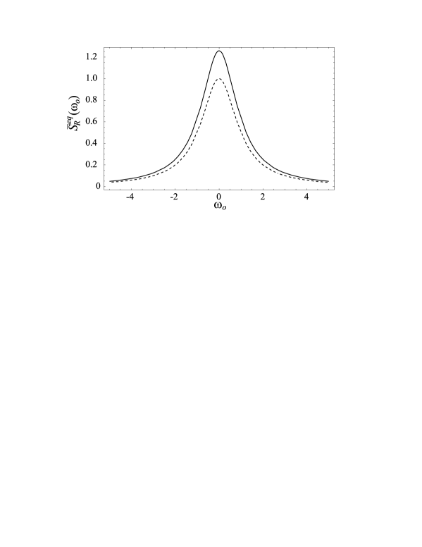
Figure 2: Normalized central peak in equilibrium, $\bar{S}_{R}^{eq}$, as function of the normalized frequency $\omega_{o}$. (—) corresponds to a compressible nematic solvent and (- - -) denotes the incompressible contribution obtained in $I$. $\bar{S}_{R}^{eq}$ is calculated from Eq. (63) for typical values of the material parameters and the scattering geometry shown in Fig. 1 with $k_{1}=1\times 10^{5}$ $cm^{-1}$ and $\theta=1^{\circ}$.

IV.1.2 Brillouin Peaks

The Brillouin peaks are located at the frequencies $\omega\simeq\pm$ $c_{s}k$ and Eqs. (19) and (53) yield the following expression for the normalized Brillouin spectrum of the impurities in terms of $\omega_{o}$

$$\bar{S}_{B}^{eq}\left(\omega_{o}\right)=\frac{1}{2}\frac{k_{B}T_{o}c_{o}}{\rho_{o}c^{2}}\Gamma_{o}\left[\frac{1}{\left(\omega_{o}+\frac{c_{s}k}{\omega_{D}}\right)^{2}+\Gamma_{o}^{2}}+\frac{1}{\left(\omega_{o}-\frac{c_{s}k}{\omega_{D}}\right)^{2}+\Gamma_{o}^{2}}\right],$$ (65)

with $\Gamma_{o}\equiv\Gamma(\overrightarrow{k})/\omega_{D}\left(\overrightarrow{k}\right)$. First, notice that the ratio of the maxima of the central and Brillouin peaks is

$$\zeta=\frac{k_{B}T_{o}c_{o}}{\rho_{o}c_{s}^{2}\Gamma_{o}}.$$ (66)

Thus, if we consider the order of magnitude of the involved parameters for the diffusion of dyes in a typical thermotropic nematic as above, it follows that $\zeta\sim 10^{-10}$. This shows that the Brilloiun component of the light scattering spectrum of the impurities is negligible when compared in front of its central part.

IV.2 Nonequilibrium Light Scattering Spectrum

We now consider the effect of the concentration gradient on the dynamic structure factor of the impurities when the solvent is in its nematic phase. It is convenient to introduce the normalized concentration gradient components by

$$\bar{a}_{i}\equiv\frac{a_{i}}{k_{1}c_{o}}.$$ (67)

IV.2.1 Central Peak

If we keep only the dominant terms Eqs. (23)-(25), for $\bar{a}_{i}$ in the range $10^{-8}<\bar{a}_{i}<1$, we obtain that at low frequencies, $\omega\simeq\omega_{D}\left(\overrightarrow{k}\right)$, $S_{vv}^{neq}\left(\overrightarrow{k},\omega\right)\gg S_{nn}^{neq}\left(\overrightarrow{k},\omega\right)\gg S_{nv}^{neq}\left(\overrightarrow{k},\omega\right)$ and the leading nonequilibrium contribution to the dynamic structure factor can then be written in the form

$$\bar{S}_{R}^{neq}\left(\omega_{o}\right)=\frac{c_{o}k_{B}T_{o}}{\rho_{o}\omega_{D}\left(\overrightarrow{k}\right)}k_{1}^{2}\frac{1}{1+\omega_{o}^{2}}\left[\frac{\bar{a}_{1}^{2}\left(\overrightarrow{k}\right)}{\omega_{v1}\left(\overrightarrow{k}\right)}+\frac{\bar{a}_{2}^{2}\left(\overrightarrow{k}\right)}{\omega_{v2}\left(\overrightarrow{k}\right)}\right].$$ (68)

Thus, in the nonequilibrium state the central peak of the dynamic structure factor, $\bar{S}_{R}=\bar{S}_{R}^{eq}+\bar{S}_{R}^{neq}$, takes the form

$$\bar{S}_{R}\left(\omega_{o}\right) = \frac{1}{1+\omega_{o}^{2}}\left\{1+\frac{c_{o}k_{B}T_{o}}{\rho_{o}c_{s}^{2}}\frac{\left(\gamma-1\right)\omega_{T}\left(\overrightarrow{k}\right)}{\omega_{D}\left(\overrightarrow{k}\right)}\right.$$ (69)

$$\left.+\frac{c_{o}k_{B}T_{o}}{\rho_{o}\omega_{D}\left(\overrightarrow{k}\right)}k_{1}^{2}\left[\frac{\bar{a}_{1}^{2}\left(\overrightarrow{k}\right)}{\omega_{v_{1}}\left(\overrightarrow{k}\right)}+\frac{\bar{a}_{2}^{2}\left(\overrightarrow{k}\right)}{\omega_{v_{2}}\left(\overrightarrow{k}\right)}\right]\right\}.$$

This result indicates that the effect of the concentration gradient increases both, the height and the half-width at half-height of the spectrum. The relative magnitude of the nonequilibrium contribution is measured by the function

$$\xi=\frac{\bar{S}_{R}-\bar{S}_{R}^{eq}}{\bar{S}_{R}^{eq}}=\frac{c_{o}k_{B}T_{o}}{\rho_{o}\omega_{D}}k_{1}^{2}\left[\frac{\bar{a}_{1}^{2}}{\omega_{v_{1}}}+\frac{\bar{a}_{2}^{2}}{\omega_{v_{2}}}\right]$$ (70)

If we take $c_{o}\sim 10^{20}$ $cm^{-3}$, $T_{o}\sim 300$ $K$, $D\sim 10^{-7}$ $cm^{2}$ $s^{-1}$, $\nu\sim 10^{-1}$ $poise$, $\rho_{o}\sim 1$ $gcm^{-3}$, $k_{1}\sim 10^{5}$ $cm^{-1}$ and small scattering angles, $\theta\sim 1{{}^{\circ}}$, a typical value is

$$\xi\sim\frac{c_{o}k_{B}T_{o}}{\rho_{o}D\nu k^{4}}k_{1}^{2}\bar{a}^{2}\sim 10^{12}\bar{a}^{2}.$$ (71)

This suggests that the nonequilibrium contribution could be significant, $\sim$ $10\%$, for normalized concentration gradients as small as $\bar{a}\sim 10^{-6}$, which are four orders of magnitude smaller than those gradients used in I. In Fig. 3 we compare $\bar{S}_{R}\left(\omega_{o}\right)$ with its equilibrium component $\bar{S}_{R}^{eq}\left(\omega_{o}\right)$ for the diffusion of dyes in the thermotropic nematic $MBBA$ at low concentrations ($5\%$), for the following specific values of the normalized concentration gradient, $a_{x}=a_{y}=0$, $a_{z}=1\times 10^{-6}$, and for the scattering process shown in Fig. 1 with $k_{1}=10^{5}$ $cm^{-1}$, $\theta=1{{}^{\circ}}$. We notice that the spectrum becomes higher and wider when the concentration gradient is present (continuos line) than in the equilibrium case (dashed line). For the considered values of the involved quantities the increment in the height is about $25\%$ and the change in the half-width at half-height is $\sim 12\%$.

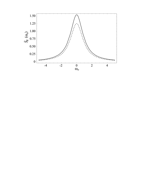
Figure 3: Normalized central peak $\bar{S}_{R}\left(\omega_{o}\right)$ as given by Eq. (69) for $k_{1}=1\times 10^{5}$ $cm^{-1}$ and $\theta=1^{\circ}$. (- - -) represents the equilibrium contribution. (—) denotes the dynamic structure factor in the $NESS$ induced by a normalized concentration gradient $\overrightarrow{a}\equiv(a_{x},a_{y},a_{z})$ with $a_{x}=a_{y}=0$, $a_{z}=1\times 10^{-6}$ ($\psi=0^{\circ}$).

IV.2.2 Brillouin Peaks

Following the same procedure, we find that the leading contribution to the nonequilibrium part of the dynamic structure factor at $\omega\simeq\pm c_{s}k$ arises from $S_{nv}^{neq}\left(\overrightarrow{k},\omega\right)$. More specifically, from the cross correlation $\left\langle\delta\tilde{n}_{3}\left(\overrightarrow{k},\omega\right)\delta\tilde{v}_{3}\left(-\overrightarrow{k},-\omega\right)\right\rangle$ and the normalized form given by (61) we get

$$\bar{S}_{B}^{neq}\left(\omega_{o}\right) = -\frac{c_{o}k_{B}T_{o}D_{a}}{\rho_{o}c_{s}^{2}k^{3}}k_{1}k_{\perp}^{2}\left[2k_{z}\overline{a}_{3}\left(\overrightarrow{k}\right)+\left(1-\left(\frac{k_{z}}{k_{\perp}}\right)^{2}\right)k_{\perp}\overline{a}_{2}\left(\overrightarrow{k}\right)\right]$$ (72)

$$\times\frac{k_{z}A\left(\overrightarrow{k}\right)\left(\gamma-1\right)\omega_{T}\left(\overrightarrow{k}\right)}{\omega_{n3}^{2}\left(\overrightarrow{k}\right)}\frac{\omega_{o}}{1+\omega_{o}^{2}},$$

where

$$A\left(\overrightarrow{k}\right) \equiv \frac{(1+\lambda)k_{z}^{2}+(1-\lambda)k_{\perp}^{2}}{\nu_{3}\left(k_{\perp}^{4}+k_{z}^{4}\right)+2\left(\nu_{1}+\nu_{2}-\nu_{3}\right)k_{\perp}^{2}k_{z}^{2}}\left[\left(2\nu_{3}+\nu_{5}-\nu_{2}-\nu_{4}\right)k_{\perp}^{2}\right.$$ (73)

$$\left.+\left(2\nu_{1}+\nu_{2}-2\nu_{3}-\nu_{4}+\nu_{5}\right)k_{z}^{2}\right].$$

Notice that the nonequilibrium term is an odd function of the frequency and, as a consequence, the external concentration gradient induces an asymmetry in the spectrum in such a way that one of its Brillouin peaks increases while the other decreases in the same amount with respect to their equilibrium counterparts. This effect is linear in the concentration gradient magnitude. Furthermore, since it can be readily shown that the function $\bar{S}_{B}^{neq}$ does not varies considerably over the frequency intervals of the order of $\Gamma\left(\overrightarrow{k}\right)$ around $\pm c_{s}k$, we can make the approximation

$$\bar{S}_{B}^{neq}\left(\omega_{o}\right) = \mp\frac{c_{o}k_{B}T_{o}D_{a}}{\rho_{o}c_{s}^{3}k^{4}}k_{1}k_{\perp}^{2}\left[2k_{z}\overline{a}_{3}+\left(1-\left(\frac{k_{z}}{k_{\perp}}\right)^{2}\right)k_{\perp}\overline{a}_{2}\right]$$ (74)

$$\times\frac{k_{z}A\left(\gamma-1\right)\omega_{T}}{\omega_{n3}^{2}},$$

where the upper sign corresponds to the peak located at $-c_{s}k$ and the lower sing to the peak at $c_{s}k$. The relative magnitude of this effect is given by the quantity

$$\chi\equiv\frac{\bar{S}_{B}-\bar{S}_{B}^{eq}}{\bar{S}_{B}^{eq}}=A\frac{k_{z}k_{1}k_{\perp}^{2}}{k^{3}}\left[2k_{z}\overline{a}_{3}+\left(1-\left(\frac{k_{z}}{k_{\perp}}\right)^{2}\right)k_{\perp}\overline{a}_{2}\right]\frac{\omega_{o}\overline{\omega}_{T}}{\omega_{n_{3}}^{2}},$$ (75)

whose significance can be estimated by taking into account the order of magnitude of the involved parameters and introducing the normalized gradient components according to (67). In this way we find that

$$\chi\sim 10^{-10}k_{1}\bar{a}\text{ }cm.$$ (76)

This implies that the nonequilibrium contribution to the Brillouin part of the spectrum could be significant only for normalized gradients of the order of $\bar{a}\sim 10^{-2}$, which are much larger than those considered for the central peak. Moreover, if the angular dependence of $\chi$ is taken into account, it turns out that this contribution is actually one order of magnitude smaller.

In order to complete our analysis we now compare the normalized Brillouin component of the dynamic structure factor of the impurities, $\bar{S}_{B}\left(\overrightarrow{k},\omega\right)$, with respect to $\bar{S}_{B}^{eq}\left(\overrightarrow{k},\omega\right)$, using the same values of the material parameters as before. For instance, for a normalized concentration gradient with components $a_{x}=a_{y}=1\times 10^{-1}$, $a_{z}=0$, and the scattering process shown in Fig. 1 with $k_{1}=10^{5}$ $cm^{-1}$ and $\theta=90{{}^{\circ}}$, the height of the Brillouin peak located at $\omega=-c_{s}k$ increases $\sim$ $7\%$ while the one located at $\omega=c_{s}k$ decreases by the same amount, as shown in Fig. 4. Finally, we stress that both, the Brillouin component of the spectrum and the nonequilibrium effect on the Brillouin peaks are several orders of magnitude smaller than the central component and the nonequilibrium effect on this peak, respectively. Thus, the possible experimental observation of the effects discussed in this work seems to be more feasible for the central component of $S\left(\overrightarrow{k},\omega\right)$.

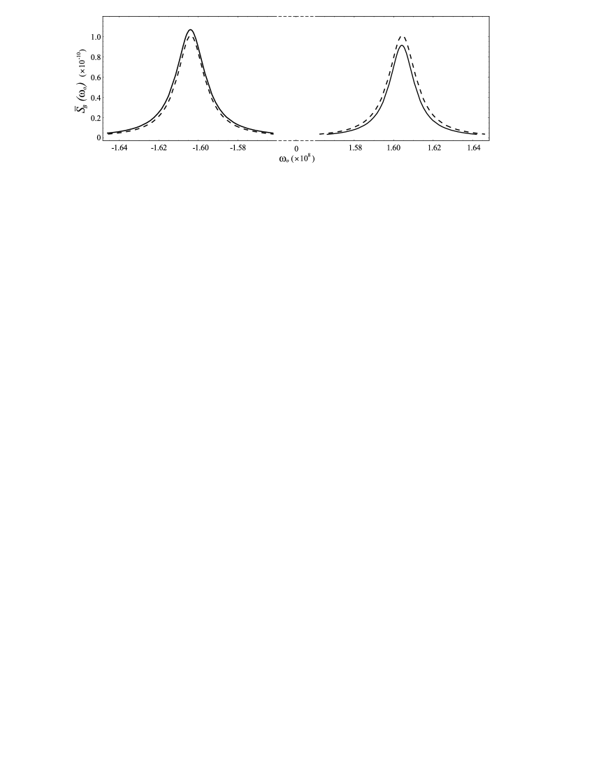
Figure 4: Normalized Brillouin spectrum $\bar{S}_{R}\left(\omega_{o}\right)$ as given by Eqs. (65) and (72) for $k_{1}=1\times 10^{5}$ $cm^{-1}$ and $\theta=90^{\circ}$. (- - -) represents the equilibrium part of the spectrum while (—) is the dynamic structure factor in the $NESS$ induced by a normalized concentartion gradient with components $a_{x}=a_{y}=1\times 10^{-1}$, $a_{z}=0$.

V Concluding Remarks

Summarizing, by using a fluctuating hydrodynamic approach we have investigated theoretically the influence of the effects produced by a uniform impurities concentration gradient on the light scattering spectrum of a suspension in a compressible nematic solvent. We compared both cases, when the solvent is in a fully thermodynamic equilibrium state and in a non-equilibrium steady state induced by a dye-concentration gradient. In the former state, the spectrum is symmetric (Lorentzian) with respect to the frequency shifts, but anisotropic through its explicit dependence on the diffusion coefficients of the dye, parallel and normal to the mean molecular axis of the nematic. The values of these coefficients were taken from experimental measurements of diffusion of methylred and nitrozo di-methyl aniline in a $MBBA$ solvent. Our results showed that the compressibility increases the height and the width at mid-height with respect to the incompressible case in amounts which vary up to $25\%$ for a dye diluted suspension at $5\%$ in $MBBA$.

As was discussed above, the nonequilibrium correction turns out to be several orders of manitude larger for the central peak of the spectrum than for the Brillouin part. The Rayleigh peak becomes higher and wider when the concentration gradient is present with respect to the equilibrium case. For the considered values of the involved quantities, the increment in the height is about $25\%$ and the change in the half-width at half-height is $12\%$, as indicated in Fig. 3. The size of this effect depends on the square of the gradient components.

To our knowledge, the physical situation dealt with here has not been considered in the literature and our model calculations yield new results that might be observable; however, this remains to be assessed.

References

• (1) H. Híjar and R. F. Rodríguez, Phys. Rev. E, 69, 051701 (2004)
• (2) D. Beysens, T. Garrabos and G. Zalczer, Phys. Rev. Lett. 48, 403 (1980)
• (3) J. R. Dorfman, T. R. Kirkpatrick and J. V. Sengers, Annu. Rev. Phys. Chem. 45, 213 (1994)
• (4) B. Law, M., P. N. Segrè, R. W. Gammon and J. V. Sengers, Phys. Rev. A 41, 816 (1990)
• (5) F. Rondelez, Sol. State Commun. 14, 815 (1974)
• (6) F. Jähnig and H. Scmidt, Ann. Phys (New York) 71, 129 (1972)
• (7) W. Franklin, Phys. Rev. A 11, 2156 (1975)
• (8) L. D. Landau and E. Lifshitz, Fluid Dynamics (Pergamon, New York, 1959)
• (9) D. Forster, Hydrodynamic Fluctuations, Broken Symmetry and Correlation Functions (Benjamin, Reading, 1975)
• (10) D. Forster, T. Lubensky, P. C. Martin, J. Swift, P. S. Pershan, Phys. Rev. Lett. 26, 1016 (1971)
• (11) R. F. Rodríguez and H. Híjar, Eur. Phys. J. B 50, 105-110 (2006)
• (12) I. C. Khoo and S. T. Wu, Optics and Nonlinear Optics of Liquid Crystals (World Scientific, Singapore, 1993)
• (13) U. Geigenmüller, U. M. Titulaer and B. U. Felderhof, Physica, 119A, 41 (1983)
• (14) U. Geigenmüller, B. U. Felderhof and U. M. Titulaer, Physica, 120A, 635 (1983)
• (15) H. Híjar, Ph. D. Dissertation, National University of Mexico (2006) (in Spanish)
• (16) J. F. Camacho, H. Híjar and R. F. Rodríguez, Physica A 348, 252 (2005)
• (17) H. Híjar and R. F. Rodríguez, Rev. Mex. Fis., (2006) (in press)
• (18) R. F. Rodríguez and J. F. Camacho, Nonequilibrium thermal light scattering from nematic liquid crystals in Recent Developments in Mathematical and Experimental Physics, Vol. B Statistical Physics and Beyond, A. Macias, E. Díaz and F. Uribe, editors (Kluwer, New York, 2002) pp. 209-224