Nonequilibrium Langevin Approach to
Quantum Optics in Semiconductor Microcavities

Abstract

Recently the possibility of generating nonclassical polariton states by means of parametric scattering has been demonstrated. Excitonic polaritons propagate in a complex interacting environment and contain real electronic excitations subject to scattering events and noise affecting quantum coherence and entanglement. Here we present a general theoretical framework for the realistic investigation of polariton quantum correlations in the presence of coherent and incoherent interaction processes. The proposed theoretical approach is based on the nonequilibrium quantum Langevin approach for open systems applied to interacting-electron complexes described within the dynamics controlled truncation scheme. It provides an easy recipe to calculate multi-time correlation functions which are key-quantities in quantum optics. As a first application, we analyze the build-up of polariton parametric emission in semiconductor microcavities including the influence of noise originating from phonon induced scattering.

I Introduction

Entanglement is one of the key features of quantum information and communication technologyNielsen-Chuang . Parametric down-conversion is the most frequently used method to generate highly entangled pairs of photons for quantum-optics applications, such as quantum cryptography and quantum teleportation. Rapid development in the field of quantum information requires monolithic, compact sources of nonclassical photon states enabling efficient coupling into optical fibres and possibly electrical injection. Semiconductor-based sources of entangled photons would therefore be advantageous for practical quantum technologies. Moreover semiconductors can be structured on a nanometer scale, and thus one may produce materials with tailored properties realizing a wide variety of physically distinct situations. However semiconductor heterostructures constitute a complex interacting environment involving charge, spin, and lattice degrees of freedom, hence suited to serve as prototype systems where quantum-mechanical properties of many interacting particles far away from equilibrium can be studied in a controlled fashionAxtKuhn . It has been demonstrated that very large $\chi^{(3)}$ resonant polaritonic nonlinearities in wide-gap semiconductors and in semiconductor microcavities can be used to achieve parametric emissionCuCl Honerlage ; Baumberg .

Polaritons are mixed quasiparticles resulting from the strongly coupled propagation of light and collective electronic excitations (excitons) in semiconductor crystals. Although spontaneous parametric processes involving polaritons in bulk semiconductors have been known for decadesCuCl Honerlage , the possibility of generating entangled photons by these processes was theoretically pointed out only latelySavasta PRL96 . This result was based on a microscopic quantum theory of the nonlinear optical response of interacting electron systems relying on the dynamics controlled truncation schemeVictor-Axt-Stahl PRB extended to include light quantizationSavasta PRL2003 ; HRS Savasta ; SSC Savasta . The above theoretical framework was also applied to the analysis of polariton parametric emission in semiconductor microcavities (SMCs)Savasta PRL2003 ; HRS Savasta . A SMC is a photonic structure designed to enhance light-matter interactions. The strong light-matter interaction in these systems gives rise to cavity polaritons which are hybrid quasiparticles consisting of a superposition of cavity photons and quantum well excitons Weisbuch-Houdre . Demonstrations of parametric amplification and parametric emission in SMCsBaumberg ; Erland ; Langbein PRB2004 , together with the possibility of ultrafast optical manipulation and ease of integration of these microdevices, have increased the interest on the possible realization of nonclassical cavity-polariton statessqueezing Quattropani ; CiutiBE ; Savasta PRL2005 ; LosannaCC ; SSC Savasta . In 2004, experimental evidence for the generation of ultraviolet polarization-entangled photon pairs by means of biexciton resonant parametric emission in a single crystal of semiconductor CuCl has been reportedNature CuCl . Short-wavelength entangled photons are desirable for a number of applications as generation of further entanglement between three or four photons. In 2005 an experiment probing quantum correlations of (parametrically emitted) cavity polaritons by exploiting quantum complementarity has been proposed and realizedSavasta PRL2005 . Specifically, it has been shown that polaritons in two distinct idler modes interfere if and only if they share the same signal mode so that which-way information cannot be gathered, according to Bohr’s quantum complementarity principle. In 2006 a promising low-threshold parametric oscillation in vertical triple SMCs with signal, pump and idler waves propagating along the vertical direction of the nanostructure has been demonstratedCiuti Nature .

The crucial role of many-particle Coulomb correlations in semiconductors marks a profound difference from dilute atomic systems, where the optical response is well described by independent transitions between atomic levels, and the nonlinear dynamics is governed only by saturation effects due to the Pauli exclusion principle. In planar SMCs, thanks to their mutual Coulomb interaction, pump polaritons generated by resonant optical pumping may scatter into pairs of polaritons (signal and idler)Savasta PRL96 ; Baumberg ; Ciuti parlum , they are determined by the two customary energy and wave vector conservation conditions $2{\bf k}_{p}={\bf k}_{s}+{\bf k}_{i}$ and $2E_{{\bf k}_{p}}=E_{{\bf k}_{s}}+E_{{\bf k}_{i}}$ depicting an eight-shaped curve in momentum space. At low pump intensities they are expected to undergo a spontaneous parametric process driven by vacuum-fluctuation, whereas at moderate intensities they display self-stimulation and oscillation Baumberg . However they are real electronic excitations propagating in a complex interacting environment. Owing to the relevance of polariton interactions, and also owing to their interest for exploring quantum optical phenomena in such a complex environment, theoretical approaches able to model accurately polariton dynamics including light quantization, losses and environment interactions are highly desired. The analysis of nonclassical correlations in semiconductors constitutes a challenging problem, where the physics of interacting electrons must be added to quantum optics and should include properly the effects of energy relaxation, dephasing, and noise, induced by electron-phonon interaction Kuhn-Rossi PRB 2005 .

Previous descriptions of polariton parametric processes make deeply use of the picture of polaritons as interacting bosons. These theories have been used to investigate parametric amplifications, parametric luminescence, coherent control, entanglement and parametric scattering in momentum spaceCiuti parAmpl ; Ciuti parlum ; LosannaCC ; CiutiBE ; Langbein PRB2004 .

It is worth noting that in a realistic environment phase-coherent nonlinear optical processes involving real excitations compete with incoherent scattering as evidenced by experimental results. In experiments dealing with parametric emission, what really dominates emission at low pump intensities is the photoluminescence (PL) due to the incoherent dynamics of the single scattering events driven by the pump itself and the Rayleigh scattering of the pump due to the unavoidable presence of structural disorder. The latter process is elastic and can thus be spectrally filtered in principle, moreover it is confined in k-space to a ring of in-plane wave vectors with almost the same modulus of the pump wave vector. On the contrary PL, being not an elastic process, cannot be easily separated from parametric emission. Only once the pumping become sufficient the parametric processes start to reveal themselves and to take over pump-induced PL as well. Indeed, usually, parametric emission and standard pump-induced PL cohabit as shown by experiments at low and intermediate excitation densityLangbein PRB2004 . Moreover, in order to address quantum coherence properties and entanglementNature CuCl the preferred experimental situations are those of few-particle regimes, namely coincidence detection in photon counting. In this regime, the presence of incoherent noise due to pump-induced PL tends to spoil the system of its coherence properties lowering the degree of nonclassical correlations. The detrimental influence of incoherent effects on the quantum coherence properties is also well evidenced in the measured time-resolved visibility shown in Ref. Savasta PRL2005, . At initial times visibility is suppressed until parametric emission prevails. Thus, a microscopic analysis able to account for parametric emission and pump-induced PL on an equal footing is highly desirable in order to make quantitative comparison with measurements and propose future experiments. Furthermore a quantitative theory would be of paramount importance for a deeper understanding of quantum correlations in such structures aiming at seeking and limiting all unwanted detrimental contributions.

The dynamics controlled truncation scheme (DCTS) provides a (widely adopted) starting point for the microscopic theory of light-matter interaction effects beyond mean-field AxtKuhn ; Victor-Axt-Stahl PRB , supplying a consistent and precise way to stop the infinite hierarchy of higher-order correlations which always appears in the microscopic approaches of manybody interacting systems. In 1996 the DCTS was extended in order to include in the description the quantization of the electromagnetic field Savasta PRL96 . This extension has been applied to the study of quantum optical phenomena in semiconductors as polariton entanglement SSC Savasta . However, in these works damping has been considered only at a phenomenological level.

In this paper we shall present a novel approach based on a DCTS-nonequilibrium quantum Langevin description of the open system in interaction with its surroundings. This approach enables us to include on an equal footing the microscopic description of the scattering channels competing with the coherent parametric phenomena the optical pump induces. We shall apply our method in order to perform a more realistic description of light emission taking into account nonlinear parametric interactions, light quantization, cavity losses and polariton-phonon interaction. The developed theoretical framework can be naturally extended to include other incoherent scattering mechanisms such as the interaction of polaritons with thermal free electrons Di Carlo Kavokin PRB . As a first application of the proposed theoretical scheme, we have analyzed the time-resolved and time-integrated build-up of polariton parametric emission in semiconductor microcavities including the influence of noise originating from phonon induced scattering. The presented numerical results clearly evidence the role of incoherent scattering in parametric photoluminescence and thus show the importance of a proper microscopic analysis able to account for parametric emission and pump-induced PL on an equal footing. We also exploit the present approach to calculate the emission spectra as a function of the pump power density. The spectra display a significant line-narrowing as well as parametric emission starts to prevail.

The paper is organized as follows. In Sec II, starting from a DCTS theory for semiconductor microcavities nostro teoria , we present a theory of $\chi^{(3)}$ optical nonlinearities in terms of interacting polaritons. The latter focuses mainly on the nonlinear part in order to model coherent optical parametric processes and the damping is included only phenomenologically. In Section III we apply a nonequilibrium quantum Langevin treatment of damping and fluctuations in an open system, originally proposed by Lax. Section IV will be devoted to the microscopic calculation of phonon-induced scattering rates and polariton PL within a second order Born-Markov approximation. In Sec. V we shall present a quantum Langevin description of parametric emission including incoherent effects; particular attention will be devoted to the case of single pump feed, whose results will be the subject of Sec. VI. Finally in Sec. VII we shall summarize and draw some conclusions.

II Dynamics Controlled Truncation Scheme for Interacting Polaritons

The system under investigation consists of one or more (uncoupled) QWs grown inside a semiconductor planar Fabry-Perot resonator. For the quasi-2D interacting electron system we adopt the usual semiconductor model Hamiltonian AxtKuhn which can be expressed as

$$\hat{H}_{e}=\sum_{N\alpha}\hbar\omega_{N\alpha}\mid{N\alpha}\rangle\langle{N\alpha}\mid\,,$$ (1)

where the eigenstates of $\hat{H}_{e}$ have been labeled according to the number N of electron-hole (eh) pairs. The state $\mid{N=0}\rangle$ is the electronic ground state, the $N=1$ subspace is the exciton subspace with the additional collective quantum number $\alpha$ denoting the exciton energy level $n$ and the in-plane wave vector ${\bf k}$. The set of states with $N=2$ determines the biexciton subspace. We treat the planar-cavity field within the quasimode approximation, the cavity field is quantized as though the mirrors were perfect:

$$\hat{H}_{c}=\sum_{k}\hbar\omega_{k}\hat{a}_{\bf k}^{{\dagger}}\hat{a}_{\bf k}\,,$$ (2)

and the resulting discrete modes are then coupled to the external continuum of modes by an effective Hamiltonian

$$\hat{H}_{p}=i\hbar\,t_{c,j}\sum_{j=1,2,\bf k}(\hat{E}^{(-)}_{j,\bf k}\hat{a}^{\dagger}_{\bf k}-\hat{E}^{(+)}_{j,\bf k}\hat{a}_{\bf k})\,,$$ (3)

where $j$ labels the two mirrors and $t_{j}$ determines the fraction of the field amplitude passing the cavity mirror, $\hat{E}^{(-)}_{j,\bf k}$ ($\hat{E}^{(+)}_{j,\bf k}$) is the positive (negative) frequency part of the coherent input light field. The coupling of the electron system to the cavity modes is given within the usual rotating wave approximation

$$\hat{H}_{I}=-\sum_{n{\bf k}}\hbar V_{n{\bf k}}\hat{a}_{\bf k}^{{\dagger}}\hat{B}_{n{\bf k}}+H.c.$$ (4)

$\hat{B}_{n{\bf k}}$ is the exciton destruction operator and can be expanded as well in terms of the energy eigenstates of the electron system. For later convenience, the exciton and photon operators are normalized so that $\hat{B}^{\dagger}_{\bf k}\hat{B}_{\bf k}$ and $\hat{a}^{\dagger}_{\bf k}\hat{a}_{\bf k}$ are operators corresponding to the number of particles within a Bohr-radius two-dimensional disk ($\pi a^{2}_{\text{x}}$) at a given ${\bf k}$.

We start from the Heisenberg equations of motion for the exciton and photon operators. In the DCTS spirit, we keep only those terms providing the lowest nonlinear response ($\chi^{(3)}$) in the input light field nostro teoria . We assume the pump polaritons driven by a quite strong coherent input field ${E}_{\bf k}^{in}=\langle\hat{E}^{(-)}_{1{\bf k}}\rangle$ consisting of a classical ($\mathbb{C}$-number) field, resonantly exciting the structure at a given energy and wave vector, $\bf{k}_{p}$. We are interested in studying polaritonic effects in SMCs where the optical response involves mainly excitons belonging to the 1S band with wave vectors close to normal incidence, $|{\bf k}|\ll\frac{\pi}{a_{\text{x}}}$. We retain only those terms containing the semiclassical pump amplitude twice, thus focusing on the “direct” pump-induced nonlinear parametric interaction. One ends up with a set of coupled equations of motion exact to the third order in the exciting field. While a systematic treatment of higher-order optical nonlinearities would require an extension of the equations of motion, a restricted class of higher-order effects can be obtained from solving these equations self-consistently up to arbitrary order as it is usually employed in standard nonlinear optics. This can be simply accomplished by replacing, in the nonlinear sources, the linear excitonic polarization and and light field operators with the total field. From now on, that the pump-driven terms (e.g. the $B$ and $a$ at ${\bf k}_{p}$) are ${\mathbb{C}}$-numbers coherent amplitudes like the semiclassical electromagnetic pump field, we will make such distinction in marking with a “hat” the operators only. It yields nostro teoria

$$\dot{\hat{B}}_{\bf k}&=-i{{\omega}}^{\text{x}}_{\bf k}\hat{B}_{\bf k}-i\hat{s}_{\bf k}+iV\hat{a}_{\bf k}-i\hat{R}^{NL}_{\bf k}\,,\\ \dot{\hat{a}}_{\bf k}=-i{{\omega}}^{c}_{\bf k}\hat{a}_{\bf k}+iV\hat{B}_{\bf k}+t_{c}{E}_{\bf k}^{in}\,\,;$$ (5)

where ${\omega}^{(i)}_{\bf k}$ ($i=\text{x},c$) are the energies of QWs excitons and cavity photons. The intracavity and the exciton field of a given mode ${\bf k}$ are coupled by the exciton-cavity photon coupling rate $V$. The relevant non-linear source term, able to couple waves with different in-plane wave vector ${\bf k}$, is given by $\hat{R}^{NL}_{\bf k}=(\hat{R}^{sat}_{\bf k}+\hat{R}^{\text{xx}}_{\bf k})/N_{eff}$; where the first term originates from the phase-space filling of the exciton transition,

$$\hat{R}^{sat}_{{\bf k}}=\frac{V}{n_{\text{sat}}}B_{{\bf k}_{p}}a_{{\bf k}_{p}}\hat{B}^{\dagger}_{{\bf k}_{i}}\,;$$ (6)

being ${n_{sat}}=7/16$ the exciton saturation density and ${\bf k}_{i}=2{\bf k}_{p}-{\bf k}$. $N_{eff}$ depends on the number of wells inside the cavity and their spatial overlap with the cavity-mode. Inserting a large number of QWs into the cavity results also in increasing the photon-exciton coupling rate $V=V_{1}\sqrt{N_{eff}}$, where $V_{1}$ is the exciton-photon coupling for 1 QW. ${\hat{R}}^{\text{xx}}_{\bf k}$ is the Coulomb interaction term. It dominates the coherent xx coupling and for co-circularly polarized waves (the only case here addressed) can be written as

$$\hat{R}^{\text{xx}}_{{\bf k}}=\hat{B}^{\dagger}_{{\bf k}_{i}}(t)\bigg{(}V_{\text{xx}}B_{{\bf k}_{p}}(t)B_{{\bf k}_{p}}(t)-$$

$$-i\int_{-\infty}^{t}dt^{\prime}F(t-t^{\prime})B_{{\bf k}_{p}}(t^{\prime})B_{{\bf k}_{p}}(t^{\prime})\bigg{)}\,,$$ (7)

where $V_{\text{xx}}\simeq 6E_{b}/\pi$, being $E_{b}$ the exciton binding energy. Equation (7) includes the instantaneous mean-field xx interaction term and a non-instantaneous term originating from four-particle correlations. These equations show a close analogy to those derived in HRS Savasta , addressing the bulk case. In addition to that former result, in the present formulation we succeed in dividing rigorously (in the DCTS spirit) the Coulomb-induced correlations into mean-field and four-particle correlation terms. Moreover the pump-induced shift due to parametric scattering $\hat{s}_{\bf k}$ reads

$$N_{eff}\hat{s}_{\bf k}=\frac{V}{n_{\text{sat}}}\bigg{(}B^{*}_{{\bf k}_{p}}a_{{\bf k}_{p}}\hat{B}_{{\bf k}}+B^{*}_{{\bf k}_{p}}B_{{\bf k}_{p}}\hat{a}_{{\bf k}}\bigg{)}+2V_{\text{xx}}B^{*}_{{\bf k}_{p}}B_{{\bf k}_{p}}\hat{B}_{{\bf k}}-$$

$$\hskip 71.13188pt-2iB^{*}_{{\bf k}_{p}}(t)\int_{-\infty}^{t}dt^{\prime}F(t-t^{\prime})\hat{B}_{{\bf k}}(t^{\prime})B_{{\bf k}_{p}}(t^{\prime})\,.$$ (8)

Equation (5) can be written in compact form as

$$\dot{\mathbf{\cal B}}_{\bf k}=-i\mathbf{\Omega}^{\text{xc}}_{\bf k}\,\mathbf{\cal B}_{\bf k}+\mathbf{\cal E}^{in}_{\bf k}-i\mathbf{{\cal R}}_{\bf k}^{NL};$$ (9)

where $\mathbf{\cal B}_{\bf k}\equiv\left(\begin{array}[]{c}\hat{B}_{\bf k}\\ \hat{a}_{\bf k}\end{array}\right)$, $\mathbf{\Omega}^{\text{xc}}_{\bf k}\equiv\left(\begin{array}[]{cc}{\omega}^{x}_{\bf k}&-V\\ -V&{\omega}^{c}_{\bf k}\end{array}\right)$, $\mathbf{\cal E}^{in}_{\bf k}\equiv\left(\begin{array}[]{c}0\\ t_{c}{E}^{in}_{\bf k}\end{array}\right)$, and $\mathbf{{\cal R}}_{\bf k}^{NL}\equiv\left(\begin{array}[]{c}\hat{R}^{NL}_{\bf k}\\ 0\end{array}\right)$. When the coupling rate $V$ exceeds the decay rate of the exciton coherence and of the cavity field, the system enters the strong coupling regime. In this regime, the continuous exchange of energy before decay significantly alters the dynamics and hence the resulting resonances of the coupled system with respect to those of bare excitons and cavity photons. As a consequence, cavity-polaritons arise as the two-dimensional eigenstates of $\mathbf{\Omega}^{\text{xc}}_{\bf k}$. The coupling rate $V$ determines the splitting ($\simeq 2V$) between the two polariton energy bands. This nonperturbative dynamics including the interactions (induced by $\hat{R}^{NL}_{\bf k}$) between different polariton modes can be accurately described by Eq.  (5). Nevertheless there can be reasons to prefer a change of bases from excitons and photons to the eigenstates of the coupled system, namely polaritons. An interesting one is that the resulting equations may provide a more intuitive description of nonlinear optical processes in terms of interacting polaritons. Moreover equations describing the nonlinear interactions between polaritons become more similar to those describing parametric interactions between photons widely adopted in quantum optics. Another, more fundamental reason, is that the standard second-order Born-Markov approximation scheme, usually adopted to describe the interaction with environment, is strongly bases-dependent, and using the eigenstates of the closed system provides more accurate results. In order to obtain the dynamics for the polariton system we perform on the exciton and photon operators the unitary basis transformation

$$\mathbf{\cal P}_{\bf k}=U_{\bf k}\mathbf{\cal B}_{\bf k};$$ (10)

being $\mathbf{\cal P}_{\bf k}=\left(\begin{array}[]{c}\hat{P}_{1{\bf k}}\\ \hat{P}_{2{\bf k}}\end{array}\right)$ and

$$U_{\bf k}=\left(\begin{array}[]{cc}X_{1{\bf k}}&C_{1{\bf k}}\\ X_{2{\bf k}}&C_{2{\bf k}}\end{array}\right)\,.$$ (11)

In general photon operators obey Bose statistics, on the contrary the excitons do not posses a definite statistics (i.e. either bosonic or fermionic), but their behaviour may be well approximated by a bosonic-like statistics in the limit of low excitation densities. Indeed

$$[\hat{B}_{n},\hat{B}^{\dagger}_{n^{\prime}}]=\delta_{n^{\prime},n}-\sum_{\bf q}\Phi^{*}_{n{\bf q}}\Phi_{n^{\prime}{\bf q}}\sum_{N,\alpha,\beta}\Biggl{(}\langle N\alpha\mid\hat{c}^{\dagger}_{{\bf q}}c_{{\bf q}}\mid N\beta\rangle+\langle N\alpha\mid\hat{d}^{\dagger}_{-{\bf q}}d_{-{\bf q}}\mid N\beta\rangle\Biggr{)}\mid N\alpha\rangle\langle N\beta\mid\,.$$ (12)

Thus, within a DCTS line of reasoning Sham PRL95 , the expectation values of these transition operators (i.e. $\mid N\alpha\rangle\langle N\beta\mid$) are at least of the second order in the incident light field, they are density-dependent contributions. Evidently all these consideration affect polariton statistics as well, being polariton linear combination of intracavity photons and excitons. As a consequence, even if polariton operators have no definite statistics, in the limit of low excitation intensites they obey approximately bosonic-like commutation rules.

Diagonalizing $\mathbf{\Omega}^{\text{xc}}_{\bf k}$:

$$U_{\bf k}\mathbf{\Omega}^{\text{xc}}_{\bf k}=\tilde{\Omega}_{\bf k}U_{\bf k}\,,$$ (13)

where

$$\tilde{\Omega}_{\bf k}=\left(\begin{array}[]{cc}{\omega}_{1{\bf k}}&0\\ 0&{\omega}_{2{\bf k}}\end{array}\right).$$

$\omega_{1,2}$ are the eigenenergy (as a function of ${\bf k})$ of the lower (1) and upper (2) polariton states. After simple algebra it is possible to obtain this relation for the Hopfield coefficients Ciuti SST :

$$X_{1{\bf k}}=-C_{2{\bf k}}^{*};\qquad C_{1{\bf k}}=X_{2{\bf k}}^{*}\,.$$ (14)

where

$$X_{1{\bf k}}=\frac{1}{\sqrt{1+\left(\frac{V}{{\omega}_{1{\bf k}}-\omega^{c}_{k}}\right)^{2}}}\qquad C_{1{\bf k}}=\frac{1}{\sqrt{1+\left(\frac{{\omega}_{1{\bf k}}-\omega^{c}_{k}}{V}\right)^{2}}}\,.$$ (15)

Introducing this transformation into Eq.  (9), one obtains

$$\dot{\mathbf{\cal P}_{\bf k}}=-i\tilde{\Omega}_{\bf k}\mathbf{\cal P}_{\bf k}+\mathbf{\tilde{\cal E}}^{in}_{\bf k}-i\mathbf{\tilde{\cal R}}_{\bf k}^{NL};$$ (16)

where $\mathbf{\tilde{\cal R}}^{NL}=U\mathbf{{\cal R}}^{NL}$, which in explicit form reads

$$\dot{\hat{P}}_{1\bf k}&=-i{{\omega}}_{1\bf k}{\hat{P}}_{1\bf k}-i{\tilde{s}_{1\bf k}}+{\tilde{E}}^{in}_{1,\bf k}-i{\tilde{R}}^{NL}_{1\bf k}\,,\\ \dot{\hat{P}}_{2\bf k}=-i{{\omega}}_{2\bf k}{\hat{P}}_{2\bf k}-i{\tilde{s}_{2\bf k}}+{\tilde{E}}^{in}_{2,\bf k}-i{\tilde{R}}^{NL}_{2\bf k}\,\,;$$ (17)

where ${\tilde{E}}^{in}_{m\bf k}=t_{c}C_{m\bf k}{E}_{\bf k}^{in}$, and ${\tilde{R}}^{NL}_{m\bf k}=X_{i\bf k}\hat{R}^{NL}_{\bf k}$, $(m=1,2)$. Such a diagonalization is the necessary step when the eigenstates of the polariton system are to be used used as the starting states perturbed by the interaction with the environment degrees of freedom Piermarocchi bottleneck . The nonlinear interaction written in terms of polariton operators reads

$$\hat{R}^{NL}_{\bf k}=\sum_{i,j,l}{\hat{P}}^{\dagger}_{i{\bf k}_{i}}(t)\int_{-\infty}^{t}g^{ijl}_{m{\bf k}}(t,t^{\prime})P_{j{\bf k}_{p}}(t^{\prime})P_{l{\bf k}_{p}}(t^{\prime})dt^{\prime}\,,$$ (18)

being

$$g_{m{\bf k}}^{ijl}(t,t^{\prime})=\frac{1}{N_{eff}}\bigg{[}\frac{V}{n_{sat}}C^{*}_{j,{\bf k}_{p}}\delta(t-t^{\prime})+$$

$$\bigg{(}V_{\text{xx}}\delta(t-t^{\prime})-iF(t-t^{\prime})\bigg{)}X^{*}_{j,{\bf k}_{p}}\bigg{]}X^{*}_{l,{\bf k}_{p}}X_{i,{\bf k}_{i}}\,.$$ (19)

The shift $\hat{s}_{\bf k}(t)$ is transformed into

$$\tilde{s}_{m\bf k}(t)=\sum_{ijl}P^{*}_{i{\bf k}_{p}}(t)\int_{-\infty}^{t}\bigg{(}h^{ijl}_{m\bf k}\delta(t-t^{\prime})-2iF(t-t^{\prime})\bigg{)}P_{j{\bf k}_{p}}(t^{\prime})\hat{P}_{l{\bf k}}(t^{\prime})dt^{\prime}\,,$$ (20)

and

$$h^{ijl}_{m\bf k}=\frac{1}{N_{eff}}X_{m\bf k}\bigg{[}\frac{V}{n_{sat}}X_{i{\bf k}_{p}}\bigg{(}C^{*}_{j,{\bf k}_{p}}X^{*}_{{l\bf k}}+X^{*}_{j{\bf k}_{p}}C^{*}_{l{\bf k}}\bigg{)}+$$

$$+2V_{\text{xx}}X_{i{\bf k}_{p}}X^{*}_{j{\bf k}_{p}}X^{*}_{l{\bf k}}\bigg{]}\,.$$ (21)

Equation (17) describes the coherent dynamics of a system of interacting cavity polaritons. The nonlinear term drives the mixing between polariton modes with different in-plane wave vectors and possibly belonging to different branches. Of course there are nonlinear optical processes involving modes of only one branchSSC Savasta ; Savasta PRL2005 . In this case it is possible to take into account only one of the two set of equations in (17) and to eliminate the summation over the branch indexes in Eq.  (18).

Equations (17) can be considered the starting point for the microscopic description of quantum optical effects in SMCs. They extend the usual semiclassical description of Coulomb interaction effects, in terms of a mean-field term plus a genuine non-instantaneous four-particle correlation, to quantum optical effects. Only the many-body electronic Hamiltonian, the intracavity-photon Hamiltonian and the Hamiltonian describing their mutual interaction have been taken into account. The proper microscopic inclusion of losses through mirrors, decoherence and noise due to environment interactions will be the main subject of the following sections.

III Quantum Langevin noise sources : Lax theorem

In order to model the quantum dynamics of the polariton system in the presence of losses and decoherence we exploit the microscopic quantum Heisenberg-Langevin approach. We choose it because of its easiness in manipulating operators differential equations, and above all, for its invaluable flexibility and strength in performing even multitime correlation calculations, so important when dealing with quantum correlation properties of the emitted light. Moreover, as we shall see in the following, it enables, under certain assumptions, a (computationally advantageous) decoupling of incoherent dynamics from parametric processes.

In the standard well-known theory of quantum Langevin noise treatment Ford ; Mandel-Wolf greatly exploited in quantum optics, one uses a perturbative description and thanks to a Markov approximation gathers the damping as well as a term including the correlation of the system with the environment. The latter arises from the initial values of the bath operators, which are assumed to behave as noise sources of stochastic nature. Normally the model considered has the form of harmonic oscillators coupled linearly to a bosonic environment. The standard statistical viewpoint is easy understood: the unknown initial values of the bath operators are considered as responsible for fluctuations, and the most intuitive idea is to assume bosonic commutation relations for the Langevin noise sources because the bath is bosonic too. Most times these commutation relations are introduced phenomenologically with damping terms taken from experiments and/or from previous works. In other contexts a microscopic calculation has been attempted using a quantum operator approach. Besides its valuable results as soon as one tries to set a microscopic calculation for interaction forms different from a 2-body linear coupling Mandel-Wolf , e.g. acoustic-phonon interaction, some problems arise and one is lead to consider additional approximations in order to close the equations of motion and obtain damping and fluctuations.

In 1966 Melvin Lax, with clear in mind the lesson of classical statistical mechanics of Brownian motion, extended the noise-source technique to quantum systems. In general, the model comprises a system of interest coupled to a reservoir (R). Considering a generic global (i.e. system+reservoirs) operator, a first partial trace over the reservoir degrees of freedom results in still a system operator, a subsequent trace over the systems degrees of freedom would give an expectation value. In order to be as clear as possible we shall denote the former operation on the environment by single brackets $\langle\ \ \rangle_{R}$, whereas for the combination of the two (partial trace over the reservoir and subsequent partial trace over the system density matrices) the usual brackets $\langle\ \ \rangle$ is used. His philosophy was that the reservoir can be completely eliminated provided that frequency shift and dissipation induced by the reservoir interactions are incorporated into the mean equations of motion, and provided that suitable operator noise sources with the correct moments are added. In Ref.  Lax he proposed for the first time that as soon as one is left with a closed set of equations of system operators for the mean motion (mean with respect to the reservoir) they can be promoted to equations for global bare operators (system+reservoir) provided to consider additive noise sources endowed by the proper statistics due to the system dynamics. He showed that in a Markovian environment these noise source operators must fulfill generalized Einstein equations which are a sort of time dependent non-equilibrium fluctuation-dissipation theorem.

If ${\bf\hat{a}}=\{\hat{a}_{1},\hat{a}_{2},\cdot\cdot\cdot\}$ is a set of system operators, and

$$\frac{d\left<\right.\hat{a}_{\mu}\left.\right>_{R}}{dt}=\left<\right.\hat{A}_{\mu}({\bf\hat{a}})\left.\right>_{R}$$ (22)

are the correct equations for the mean, then one can show that the equations

$$\frac{d\hat{a}_{\mu}}{dt}=\hat{A}_{\mu}({\bf\hat{a}})+\hat{F}_{\mu}({\bf\hat{a}},t)$$ (23)

are a valid set of equations of motion for the operators provided the additive noise operators $\hat{F}$’s to be endowed with the correct statistical properties to be determined for the motion itself.

The Langevin noise source operators are such that their expectation values $\langle\hat{\mathcal{F}}_{\mu}\rangle_{R}$ vanish, but their second order moments do not Lax . They are intimately linked up with the global dissipation and in a Markovian environment they take the form:

$$\langle\hat{\mathcal{F}}_{\mu}(t)\hat{\mathcal{F}}_{\nu}(u)\rangle_{R}=2\langle\hat{D}_{\mu\nu}\rangle_{R}\,\delta(t-u)\,,$$ (24)

where the diffusion coefficients are

$$2\langle\hat{D}_{\mu\nu}\rangle_{R}=\frac{d}{dt}\langle\hat{a}_{\mu}(t)\hat{a}_{\nu}(t)\rangle_{R}-\langle{\Big{\{}}\frac{d}{dt}\hat{a}_{\mu}{\Big{\}}}\hat{a}_{\nu}\rangle_{R}-\langle\hat{a}_{\mu}{\Big{\{}}\frac{d}{dt}\hat{a}_{\nu}{\Big{\}}}\rangle_{R}\,,$$ (25)

$${\Big{\{}}\frac{d}{dt}\hat{a}_{\nu}{\Big{\}}}\equiv\frac{d}{dt}\hat{a}_{\nu}-\hat{\mathcal{F}}_{\nu}\,.$$ (26)

Equation (24) is an (exact) time dependent Einstein equation representing a fluctuation-dissipation relation valid for nonequilibrium situations, it witnesses the fundamental correspondence between dissipation and noise in an open system. $\langle\hat{D}_{\mu\nu}\rangle_{R}$ becomes not only time-dependent, it is a system operator and can be seen as the extent to which the usual rules for differentiating a product is violated in a Markovian system. Equation (24) and Eq.  (25) make the resulting “fluctuation-dissipation” relations between $\hat{D}_{\mu\nu}$ and the reservoir contributions to be in precise agreement with those found by direct use of perturbation theory. This method, however, guarantees the commutation rules for the corresponding operators to be necessarily preserved in time. This result is more properly an exact, quantitative, theorem which gives relevant insights regarding the intertwined microscopic essence of damping and fluctuations in any open system.

In order to be more specific, let us consider a single semiclassical pump feed resonantly exciting the lower polariton branch at a given wave vector ${\bf k}_{p}$. It is worth noticing, however, that the generalization to a many-classical-pumps settings is straightforward. The nonlinear term $R^{NL}$ of Eq.  (18) couples pairs of wave vectors, let’s say ${\bf k}$, the signal, and ${\bf k}_{i}=2{\bf k}_{p}-{\bf k}$, the idler. A general result for quantum systems interacting with a Markovian environment is that after tracing over the bath degrees of freedom ones remains with system equations of motion in the bence of the environment plus additional phase-shifts (often neglected) and relaxation terms Lax . The Heisenberg Eqs.  (17), involving system operators, for the generic couple read

$$\frac{d}{dt}\langle\hat{P}_{\bf k}\rangle_{R}=-i\tilde{\omega}_{\bf k}\langle\hat{P}_{\bf k}\rangle_{R}+g_{\bf k}\langle\hat{P}^{{\dagger}}_{\bf k_{i}}\rangle_{R}\mathcal{P}^{2}_{{\bf k}_{p}}$$

$$\frac{d}{dt}\langle\hat{P}^{\dagger}_{\bf k_{i}}\rangle_{R}=i\tilde{\omega}_{\bf k_{i}}\langle\hat{P}^{\dagger}_{\bf k_{i}}\rangle_{R}+g^{*}_{\bf k_{i}}\langle\hat{P}_{\bf k}\rangle_{R}\mathcal{P}^{2}_{{\bf k}_{p}}\,,$$ (27)

where we changed slightly the notation to underline that pump polariton amplitudes $\mathcal{P}_{{\bf k}_{p}}$ are regarded as classical variables (${\mathbb{C}}$-numbers), while the generated signal and idler polaritons are regarded as true quantum variables.

The nonlinear interaction terms in Eq.  (III) reads

$$g_{\bf k}=\frac{-i}{N_{eff}}\bigg{[}\frac{V}{n_{sat}}C^{*}_{{\bf k}_{p}}+V_{\text{xx}}X^{*}_{{\bf k}_{p}}\bigg{]}X_{{\bf k}_{p}}X^{*}_{{\bf k}_{p}}X_{{\bf k}_{i}}\,.$$ (28)

It accounts for a pump-induced blue-shift of the polariton resonances and a pump-induced parametric emission. In Eqs.  (III) only nonlinear terms arising from saturation and from the mean-field Coulomb interaction have been included. Correlation effects beyond mean-field introduce non-instantaneous nonlinear terms. They mainly determine an effective reduction of the mean-field interaction and an excitation induced dephasing. It has been shown Savasta PRL2003 that both effects depends on the sum of the energies of the scattered polariton pairs. While the effective reduction can be taken into account simply modifying $V_{\text{xx}}$, the proper inclusion of the excitation induced dephasing requires the explicit inclusion into the dynamics of four-particle states with their phonon-induced scattering and relaxation. In the following we will neglect this effect that is quite low at zero and even less at negative detuning on the lower polariton branch Savasta PRB2001 . The renormalized complex polariton dispersion $\tilde{\omega}_{\bf k}$ includes the effects of relaxation and pump-induced renormalization, $\tilde{\omega}_{\bf k}=\omega_{{\bf k}}-i\Gamma^{(\text{tot})}_{\bf k}/{2}+h_{\bf k}\left|\mathcal{P}_{{\bf k}_{p}}\right|^{2}\,,$ and

$$h_{\bf k}=\frac{1}{N_{eff}}\big{(}\frac{V}{n_{sat}}C^{*}_{{\bf k}_{p}}X_{{\bf k}_{p}}\left|X_{\bf k}\right|^{2}+\frac{V}{n_{sat}}C^{*}_{{\bf k}}X_{\bf k}\left|X_{{\bf k}_{p}}\right|^{2}$$

$$+2V_{\text{xx}}\left|X_{{\bf k}_{p}}\right|^{2}\left|X_{{\bf k}}\right|^{2}\big{)}\,.$$ (29)

The damping term $\Gamma^{(\text{tot})}_{\bf k}$ here can be regarded as a result of a microscopic calculation including a thermal bath (see next Sect.).

Following Lax’s prescription we can promote Eqs.  (III) to global bare-operator equations

$$\frac{d}{dt}\hat{P}_{\bf k}=-i\tilde{\omega}_{\bf k}\hat{P}_{\bf k}+g_{\bf k}\hat{P}^{{\dagger}}_{\bf k_{i}}\mathcal{P}^{2}_{{\bf k}_{p}}+\hat{\mathcal{F}}_{\hat{P}_{\bf k}}$$

$$\frac{d}{dt}\hat{P}^{\dagger}_{\bf k_{i}}=i\tilde{\omega}_{\bf k_{i}}\hat{P}^{\dagger}_{\bf k_{i}}+g^{*}_{\bf k_{i}}\hat{P}_{\bf k}\mathcal{P}^{2}_{{\bf k}_{p}}+\hat{\mathcal{F}}_{\hat{P}^{\dagger}_{\bf k_{i}}}\,.$$ (30)

However, in this form it is not a ready-to-use ingredient, indeed its implementation in calculating spectra and/or higher order correlators would be problematic because the noise commutation relations ask for the solution of the same (at best of an analogous) kinetic problem to be already at hand. This point can be very well explained as soon as one is interested in calculating $\langle\hat{P}^{\dagger}_{{\bf k}}\hat{P}_{{\bf k}}\rangle$, i.e. the polariton occupation, where the mere calculation is self-explanatory. We shall need

$$2\langle\hat{D}_{P^{\dagger}_{\bf k}P_{\bf k}}\rangle_{R}=\frac{d}{dt}\langle\hat{P}^{\dagger}_{\bf k}\hat{P}_{\bf k}\rangle_{R}-\langle{\Big{\{}}\frac{d}{dt}\hat{P}^{\dagger}_{\bf k}{\Big{\}}}\hat{P}_{\bf k}\rangle_{R}-\langle\hat{P}^{\dagger}_{\bf k}{\Big{\{}}\frac{d}{dt}\hat{P}_{\bf k}{\Big{\}}}\rangle_{R}\,,$$ (31)

and the diffusion coefficient for the two operators in reverse order. Thanks to the structure above we can easily see that all the coherent contributions cancel out and only the incoherent ones are left. Anyway the important fact for the present purpose is that they are proportional to the polaritonic occupation, these coefficients will be explicitly calculated in Section V.

The general solution of Eqs.  (III) in the pump reference frame reads:

$$\mathbf{P}(t)=e^{\int_{0}^{t}{\mathbf{\cal M}(t^{\prime})}dt^{\prime}}\mathbf{P}(0)+\int_{0}^{t}e^{\int_{t^{\prime}}^{t}\mathbf{\cal M}(t^{\prime\prime})dt^{\prime\prime}}\mathbf{\cal K}(t^{\prime})\,dt^{\prime}$$

$$\mathbf{P}(t)=\left(\begin{array}[]{c}\hat{P}_{\bf k}(t)\\ \hat{\overline{P}}^{\dagger}_{\bf 2k_{p}-k}(t)\end{array}\right),\mathbf{\cal K}=\left(\begin{array}[]{c}{\hat{\mathcal{F}}}_{\hat{P}_{s\bf k}}\\ {\mathcal{\hat{\overline{F}}}}_{\hat{P}^{\dagger}_{i\bf 2k_{p}-k}}\end{array}\right)$$ (36)

$$\mathbf{\cal M}=\left(\begin{array}[]{cc}\overline{\omega}_{\bf k}&\Delta({\bf k},\tau)\\ \Delta^{*}({\bf k},\tau)&\overline{\omega}^{*}_{2{\bf k}_{p}-{\bf k}}\end{array}\right)\,,$$ (39)

where

$$\overline{\omega}_{\bf k}=-i\tilde{\omega}_{\bf k}\,,$$

$$\overline{\omega}_{2{\bf k}_{p}-{\bf k}}=-i(\tilde{\omega}_{2{\bf k}_{p}-{\bf k}}-2\tilde{\omega}_{{\bf k}_{p}})\,,$$

$$\text{the pump is}\ \ \mathcal{P}_{\bf k_{p}}=\mathcal{P}^{o}_{\bf k_{p}}e^{-i\omega^{(h)}_{\bf k_{p}}t}\,,$$

$$\hat{\overline{P}}^{\dagger}_{2\bf{k_{p}-k}}=\hat{P}^{\dagger}_{2\bf{k_{p}-k}}e^{-i2\omega^{(h)}_{\bf{k_{p}}}t}\,,$$

$$\hat{\mathcal{\overline{F}}}_{\hat{P}^{\dagger}_{2\bf{k_{p}-k}}}=\hat{\mathcal{F}}_{\hat{P}^{\dagger}_{2\bf{k_{p}-k}}}e^{-i2\omega^{(h)}_{\bf{k_{p}}}t}\,,$$

$$\omega^{(h)}_{\bf k}=\omega_{{\bf k}}+h_{\bf k}\left|\mathcal{P}_{\bf k_{p}}\right|^{2}\,,$$

$$\Delta({\bf k},\tau)=g_{\bf k}\mathcal{P}^{o\ 2}_{\bf k_{p}}\,.$$ (40)

Equation (III) can be written in a more explicit form by exploiting the following identity:

$$e^{\int^{t_{2}}_{t_{1}}A(t)dt}=\alpha_{1}(t1,t2)\int^{t_{2}}_{t_{1}}A(t)dt+\alpha_{0}(t1,t2)\mathbb{I}$$

$$\alpha_{0}(t1,t2)=\frac{\Lambda_{+}(t1,t2)e^{\Lambda_{-}(t1,t2)}-\Lambda_{-}(t1,t2)e^{\Lambda_{+}(t1,t2)}}{\Lambda_{+}(t1,t2)-\Lambda_{-}(t1,t2)}$$

$$\alpha_{1}(t1,t2)=\frac{e^{\Lambda_{+}(t1,t2)}-e^{\Lambda_{-}(t1,t2)}}{\Lambda_{+}(t1,t2)-\Lambda_{-}(t1,t2)}$$

$$\Lambda_{\pm}(t1,t2)=\int^{t_{2}}_{t_{1}}\lambda_{\pm}(\tau)d\tau$$

$$\int^{t_{2}}_{t_{1}}\text{diag}[A(t)]dt=\left(\begin{array}[]{cc}\Lambda_{-}(t1,t2)&0\\ 0&\Lambda_{+}(t1,t2)\end{array}\right)$$ (43)

$$\lambda_{\pm}=w^{+}\pm\sqrt{(w^{-})^{2}+|\Delta|^{2}}$$

$$w^{+}=\frac{(\overline{\omega}_{\bf k}+\overline{\omega}^{*}_{2{\bf k}_{p}-{\bf k}})}{2},\ \ w^{-}=\frac{(\overline{\omega}_{\bf k}-\overline{\omega}^{*}_{2{\bf k}_{p}-{\bf k}})}{2}\,.$$ (44)

Eq.  (III) with Eq.  (III) provides an easy and general starting point for the calculation of multi-time correlation functions which are key-quantities in quantum optics. Taking the expectation values of the appropriate products it yields

$$\langle\hat{P}^{\dagger}_{{\bf k}}\hat{P}_{{\bf k}}\rangle=|c_{1}(0,t)|^{2}\langle\hat{P}^{\dagger}_{{\bf k}}\hat{P}_{{\bf k}}\rangle(0)+|c_{2}(0,t)|^{2}\langle\hat{P}_{{\bf k}}\hat{P}^{\dagger}_{{\bf k}}\rangle(0)+$$

$$+\int^{t}_{0}d\tau|c_{1}(\tau,t)|^{2}2\langle\hat{D}_{P^{\dagger}_{\bf k}P_{\bf k}}\rangle(\tau)+\int^{t}_{0}d\tau|c_{2}(\tau,t)|^{2}2\langle\hat{D}_{P_{\bf k}P^{\dagger}_{\bf k}}\rangle\,,$$ (45)

here

$$c_{1}(t_{1},t_{2})=\alpha_{1}(t1,t2)\int^{t_{2}}_{t_{1}}d\tau(-\frac{\Gamma_{\bf k}^{(tot)}}{2}-i\omega^{(h)}_{\bf k})+\alpha_{0}(t1,t2)$$

$$c_{2}(t_{1},t_{2})=\alpha_{1}(t1,t2)\int^{t_{2}}_{t_{1}}d\tau\Delta({\bf k},\tau)\,.$$ (46)

The two diffusion coefficients are proportional to the polariton occupation, i.e. we need as known input sources the very quantities we are about to calculate and a self-consistent solution seems unavoidable. Concluding, even if exact, Lax’s theorem is of no immediate use for it simply rearranges the various ingredients to the microscopic dynamics in a different way. It seems worth noticing however that what up to now appears as a very formal and academic line of reasoning will be the clue for all the subsequent physical arguments ending up into an innovative approach to quantum optics in the strong coupling regime. Indeed, as we shall see in Sect.  V, under certain assumptions we will be able to overcome the above mentioned difficulty elaborating a (computationally advantageous) decoupling of incoherent dynamics from parametric processes.

Anyway, it is the structure of Eq.  (31) for the diffusion coefficients which allows, physically speaking, to account for each contribution in its best proper way recognizing easily the dominant contribution. Indeed, reconsidering Eq.  (31) in the light of the proper kinetic equation for the polariton population dynamics — the subject of the following section —, it is very clear that thanks to its structure all the coherent contributions cancel out automatically giving us an easy way to separate coherent and incoherent parts, but at the same time to treat them on an equal footing when calculating the final result.

IV Microscopic Markov calculation of Polariton Photoluminescence

Excitonic polaritons propagate in a complex interacting environment and contain real electronic excitations subject to scattering events and noise, mainly originating from the interaction with lattice vibrations, affecting quantum coherence and entanglement. For a realistic description of the physics in action, we need to build up a microscopic model taking into account on an equal footing nonlinear interactions, light quantization, cavity losses and polariton-phonon interaction. To be more specific as a dominant process for excitonic decoherence in resonant emission from QWs we shall consider acoustic-phonon scattering via deformation potential interaction, whereas we shall model the losses through the cavity mirrors within the quasi-mode approach (see Appendix  A). It is worth pointing out that the approach we are proposing may be easily enriched by several other scattering mechanisms suitable for a refinement of the numerical results.

In the view of the change of bases previously-mentioned, so imperative for a proper Markov calculation, we decide to treat the coupled system, described by the three Hamiltonian terms $\hat{H}_{e}$, $\hat{H}_{c}$ and $\hat{H}_{I}$, as our system of interest weakly interacting with the environment. In practice, this means to start from the linear part of the Heisenberg equations of motion in Eq.  (5), which can be considered in the spirit of Sect.  III as system-operator equations, without the input term. Once obtained the polariton modes via a unitary diagonalizing transformation Eq.  (13), we apply, to the coupling of this system with the environment, the usual many-body perturbative description. We end up with the customary Bogoliubov-Born-Green-Kirkwood-Yvon (BBGKY) hierarchy which to the first order gives us the coherent input field, whereas to the second order the phonon and radiative scattering terms. As widely used in the literature, we shall limit ourselves up to this point thus performing a second-order Born-Markov description of the environment induced effects to the system dynamics. To exemplify our approach we shall calculate the relaxation rate of $\langle\hat{O}\rangle=\langle\hat{P}^{\dagger}_{\alpha{\overline{\bf k}}}\hat{P}_{\alpha\overline{\bf k}}\rangle$ in the sole case of acoustic phonon interaction, any other scattering mechanism will be treated in the same way. The rate equation governing the incoherent dynamics to the lowest order of the polariton occupation is a relevant quantity we exploit in the next Sect. when we propose our DCTS-Langevin recipes for the calculation of multi-time many-body correlation functions. Being the full trace of the polariton density over the reservoir and the system degrees of freedom a relevant physical observable that we need to solve numerically, we prefer to give explicitly full account of the manipulations we have followed. It is worth underline that the very same formal treatment, i.e. Markov approximation, can be performed easily on the system operator arisen form the partial trace over the reservoir density matrix, $\langle\ \ \rangle_{R}$ Lax . In this latter guise damping and dephasing enter the mean system operator equation (22), starting point for the Lax’s theory of quantum noise Lax . A completely analogous procedure can be followed for the calculation of the dephasing rate of $\langle\hat{P}_{\alpha\overline{\bf k}}\rangle$.

In the following the DCTS description of the interaction with the environment is limited to the lowest order. This means that effects like final state stimulation of scattering events are neglected. At the lowest order, the acoustic phonon interaction Hamiltonian can be expressed only in terms of excitonic operators as Takagahara

$$H^{DF}_{exc-ph}= \sum_{\bf q}\left(\sum_{\bf k}t^{\bf q}_{\bf k}\mid 1S\,{\bf k+q^{\|}}\rangle\langle 1S\,{\bf k}\mid\right)\left(b_{\bf q}+b^{\dagger}_{-{\bf q}}\right)=$$ (47)

$$=\sum_{\bf q}Q_{\bf q}F_{\bf q}+Q_{\bf q}F^{\dagger}_{-\bf q}\,,$$

$t^{\bf q}_{\bf k}$ is described in the Eq.  (74) of the Appendix. Simbolically $\hat{H}^{S}$ stands for all the system Hamiltonians, i.e. free dynamics and parametric scattering. The standard microscopic perturbative calculation Lax gives:

$$\frac{d}{dt}\langle\hat{O}\rangle=\left<\right.\frac{1}{i\hbar}\left[\hat{O},\hat{H}^{S}\right]\left.\right>-\frac{1}{\hbar^{2}}\sum_{\bf q,\pm}\int^{\infty}_{0}du\left(n^{R}_{\mp\bf q}+\theta(\pm)\right)$$

$$\times{\Big{(}}e^{\pm\frac{\epsilon^{R}_{\bf q}u}{i\hbar}}\left<\right.\left.\right[\hat{O},\hat{Q}_{\bf q}\left.\right]\hat{Q}_{-\bf q}(-u)\left.\right>-e^{\mp\frac{\epsilon^{R}_{-\bf q}u}{i\hbar}}\left<\right.\hat{Q}_{-\bf q}(-u)\left.\right[\hat{O},\hat{Q}_{\bf q}\left.\right]\left.\right>{\Big{)}}\,,$$ (48)

where the meaning of the new symbols are self-evident.

Within the strong coupling region, the dressing carried by the nonperturbative coupling between excitons and cavity photons highly affects the scattering and for a microscopic calculation we are urged to leave the couple picture of Eqs.  (5) and move our steps into the polaritonic operator bases. Our aim is to produce a microscopic description of damping and fluctuation and to apply it in experiments with low and-or moderate excitation intensities, thus we expect the strong-coupling regime to become crucial in the scattering rates mainly through the polaritonic spectrum. In the spirit of the DCTS we shall consider them as transitions over the polaritonic bases obtained form excitons and cavity modes states and the linear diagonalizing transformation Eq.  (13), form exciton and photon operators to polariton operators, can then be rewritten as

$$\mid 1S\,{\bf k}^{\prime}\rangle\langle 1S\,{\bf k}\mid=\sum_{i,j}X_{i{\bf k}^{\prime}}X^{*}_{j{\bf k}}\mid i{\bf k}^{\prime}\rangle\langle j{\bf k}\mid\,,$$ (49)

where it is understood we have transition operators on the left-hand side representing excitons, whereas on the right-hand side polaritons. Within the Born-Markov description we are left with

$$\frac{d}{dt}\langle\hat{P}^{\dagger}_{\alpha\overline{{\bf k}}}\hat{P}_{\alpha\overline{{\bf k}}}\rangle_{\left|{}_{H^{DF}_{exc-ph}}\right.}=-\Gamma^{ph}_{\alpha,\overline{{\bf k}}}\langle\hat{P}^{\dagger}_{\alpha\overline{{\bf k}}}\hat{P}_{\alpha\overline{{\bf k}}}\rangle+\sum_{l{\bf k^{\prime}}}W_{(\alpha\overline{{\bf k}}),(l{\bf k^{\prime}})}\langle\hat{P}^{\dagger}_{l{\bf k^{\prime}}}\hat{P}_{l{\bf k^{\prime}}}\rangle\,,$$ (50)

with

$$W^{\pm}_{(s{\bf k}),(r{\bf k^{\prime}})}=\frac{2\pi}{\hbar}\sum_{q_{z}}\left|\right.t^{{\bf k}^{\prime},q_{z}}_{\bf k}\left.\right|^{2}\left|\right.X_{s{\bf k}}\left.\right|^{2}\left|\right.X_{r{\bf k}^{\prime}}\left.\right|^{2}$$

$$\hskip 113.81102pt\delta(\epsilon_{s{\bf k}}-\epsilon_{r{\bf k}^{\prime}}\pm\hbar\omega^{R}_{({\bf k}^{\prime}-{\bf k},q_{z})})\left(\right.n_{({\bf k}^{\prime}-{\bf k},q_{z})}+\frac{1}{2}\pm\frac{1}{2}\left.\right)$$

$$W_{(s{\bf k}),(r{\bf k^{\prime}})}=\sum_{\pm}W^{\pm}_{(s{\bf k}),(r{\bf k^{\prime}})}$$

$$\Gamma^{(ph)}_{s,{\bf k}}=\sum_{r{\bf k}^{\prime}}W_{(r{\bf k^{\prime}}),(s{\bf k})}\,.$$ (51)

These happen to be the same ingredients used in Ref.  Piermarocchi bottleneck studying bottleneck effect in relaxation and photoluminescence of microcavity polaritons within a bosonic Boltzmann approach.

Within the quasi-mode approach, the emitted light is proportional to the intracavity photon number ($t_{c}$ is the transmission coefficient):

$$I_{\bf k}^{PL}(t)=t_{c}^{2}\langle\hat{a}^{\dagger}_{\bf k}\hat{a}_{\bf k}\rangle(t)=t_{c}^{2}\sum_{i}|C_{i{\bf k}}|^{2}\langle\hat{P}^{\dagger}_{i{\bf k}}\hat{P}_{i{\bf k}}\rangle(t)\,.$$ (52)

By applying the whole machinery, when including only the lowest order terms in the input light field, the following equation for the polariton-occupations dynamics is obtained:

$$\frac{d}{dt} \langle\hat{P}^{\dagger}_{i{\bf k}_{i}}\hat{P}_{i{\bf k}_{i}}\rangle=-(\Gamma^{ph}_{i,{\bf k}_{i}}+\gamma^{(c)}_{i,{\bf k}_{i}})\langle\hat{P}^{\dagger}_{i{\bf k}_{i}}\hat{P}_{i{\bf k}_{i}}\rangle$$

$$+g_{i,{\bf k}_{i}}+\Gamma^{(c)}_{i,{\bf k}_{i}}+\sum_{l{\bf k^{\prime}}}W_{(i{\bf k}_{i}),(l{\bf k^{\prime}})}\langle\hat{P}^{\dagger}_{l{\bf k^{\prime}}}\hat{P}_{l{\bf k^{\prime}}}\rangle\,,$$

with the generation rate given by

$$g_{i,\bf k}={\Big{[}}t_{c}C_{{\bf k}_{p}}E^{in(+)}_{{\bf k}}\delta_{{\bf k},{\bf k}_{p}}\langle\hat{P}^{\dagger}_{i,{\bf k}}\rangle_{coh}+t_{c}C^{*}_{{\bf k}_{p}}E^{in(-)}_{{\bf k}}\delta_{{\bf k},{\bf k}_{p}}\langle\hat{P}_{i,{\bf k}}\rangle_{coh}{\Big{]}}\,.$$ (54)

The phonon-emission $(+)$ and phonon-absorbtion $(-)$ scattering rates read

$$W^{\pm}_{(j{\bf k}^{\prime}),(i{\bf k})} =\frac{1}{\rho uS}\frac{|k^{\prime}-k|^{2}+(q^{0}_{z})2}{|\hbar uq^{0}_{z}|}|\Xi|^{2}$$

$$\times|X_{j\bf k^{\prime}}|^{2}|X_{i\bf k}|^{2}[n^{(ph)}(E^{ph}_{(k^{\prime}-k,q^{0}_{z})})+\frac{1}{2}\pm\frac{1}{2}]\,,$$

the 3D phonon wave vector is $({\bf q},q^{0}_{z})$, whereas $q^{0}_{z}$ is calculated so that the energy conservation delta function $\delta(\hbar\omega_{j{k^{\prime}}}-\hbar\omega_{i{k}}\pm E^{ph}_{\bf q})$ is satisfied,

$$\Xi=\left(D_{c}I^{\bot}_{e}(q_{z})I^{\|}_{e}({\bf k^{\prime}-k})-D_{v}I^{\bot}_{h}(q_{z})I^{\|}_{h}({\bf k^{\prime}-k})\right)\,,$$ (56)

with the overlap integrals

$$I^{\|}_{e(h)}({\bf q})=\left[1+\left(\frac{m_{h(e)}}{2(m_{e}+m_{h})}|{\bf q}|a_{\text{x}}\right)2\right]^{-3/2},$$

$$I^{\bot}_{e(h)}(q_{z})=\int_{L}dz|\chi_{e(h)}(z)|^{2}e^{iq_{z}z}\,.$$ (57)

We shall treat the cavity field in the quasi-mode approximation, that is to say we shall quantize the field as the mirror were perfect and subsequently we shall couple the cavity with a statistical reservoir of a continuum of external modes. This way on an equal footing we shall provide the input coherent driving mechanism (at first order in the interaction) and the radiative damping channel (within a second order Born-Markov description).

The escape rate through the two mirrors ($l\equiv$left, $r\equiv$right) is

$$\gamma^{(c)}_{i,{\bf k^{\|}}}=\frac{2\pi}{\hbar}|C_{i,{\bf k^{\|}}}|^{2}\sum_{s=l,r}\!\!\!\int d\omega\delta\left(\Omega^{qm}_{\bf k^{\|}}[\omega]-\omega_{k^{\|}}\right)\hbar|g_{s\bf k^{\parallel}}(\omega)|^{2}\,,$$ (58)

and the corresponding noise term reads

$$\Gamma^{(c)}_{i,{\bf k^{\|}}}=\frac{2\pi}{\hbar}|C_{i,{\bf k^{\|}}}|^{2}\sum_{s=l,r}\!\!\!\int d\omega n^{qm}_{\bf k^{\|}}(\omega)\delta\left(\Omega^{qm}_{\bf k^{\|}}[\omega]-\omega_{k^{\|}}\right)\hbar|g_{s\bf k^{\parallel}}(\omega)|^{2}\,.$$ (59)

V DCTS-Nonequilibriun Quantum Langevin approach to parametric emission

As already discussed, Eq.  (III) with Eq.  (III) provides an easy and general starting point for the calculation of multi-time correlation functions which are key-quantities in quantum optics. Thus it would be easy-tempting to wonder if, through some appropriate, thought and motivated physical considerations, we were given the noise sources as known inputs. Thanks to the structure of Eq.  (31) for the diffusion coefficients we are allowed, physically speaking, to recognize properly the dominant contribution. In order to be more specific let us fix our attention on the explicit form of $2\langle\hat{D}_{P^{\dagger}_{\bf k}P_{\bf k}}\rangle$:

$$2\langle\hat{D}_{P^{\dagger}_{\bf k}P_{\bf k}}\rangle(t)=\sum_{\bf k^{\prime}}W_{{\bf k},{\bf k}^{\prime}}\langle\hat{P}^{\dagger}_{\bf k^{\prime}}\hat{P}_{\bf k^{\prime}}\rangle(t)+\Gamma^{c}_{\bf k}\,.$$ (60)

Inspecting Eq.  (IV), it results that in the low and intermediate excitation regime the main incoherent contribution to the dynamics is the PL the pump produces by itself, the effects on the PL of subsequent pump-induced repopulation arising from the nonlinear parametric part is negligible, that is to say the occupancies of the couple signal-idler are at least one order of magnitude smaller than the pump occupancy. This means that in Eq.  (60) we can consider at the right hand side the solution in time of Eq.  (IV), i.e. only incoherent lowest order contributions. The other important diffusion coefficient reads:

$$2\langle\hat{D}_{P_{\bf k}P^{\dagger}_{\bf k}}\rangle(t) =\sum_{\bf k^{\prime}}W_{{\bf k},{\bf k}^{\prime}}\langle\hat{P}_{\bf k^{\prime}}\hat{P}^{\dagger}_{\bf k^{\prime}}\rangle(t)+\Gamma^{c}_{\bf k}+\gamma^{c}_{\bf k}=$$ (61)

$$=\sum_{\bf k^{\prime}}W_{{\bf k},{\bf k}^{\prime}}\left(\right.\langle\hat{P}^{\dagger}_{\bf k^{\prime}}\hat{P}_{\bf k^{\prime}}\rangle(t)+1\left.\right)+\Gamma^{c}_{\bf k}+\gamma^{c}_{\bf k}\,.$$

We decide to use a sort of bosonic-like commutation relation in the equation above but only in the present situation, restricted only to this precise case and to the noisy background $\langle\hat{P}_{\bf k}\hat{P}^{\dagger}_{\bf k}\rangle(0)$, responsible for spontaneous parametric emission. The reason is many-fold. The two terms, Eq.  (61) and the above noise background, will enter in Eq.  (III) multiplied by $|c_{2}|^{2}$ which contains the pump already twice. As a consequence their contribution must be to linear order. Besides, Eq.  (IV) can be considered as the very low density limit of the rate equation obtained from the picture of polaritons as bosons as obtained in Ref.  Piermarocchi bottleneck . It witnesses that when the focus is devoted to the sole incoherent lowest order dynamics, bosonic commutation rules for polaritons may be employed, though carefully. Moreover, direct computation for normal incidence gives

$$[\hat{B}_{n},\hat{B}^{\dagger}_{n^{\prime}}]=\delta_{n^{\prime},n}-\sum_{\bf q}\Phi^{*}_{n{\bf q}}\Phi_{n^{\prime}{\bf q}}\sum_{N,\alpha,\beta}\Biggl{(}\langle N\alpha\mid\hat{c}^{\dagger}_{{\bf q}}c_{{\bf q}}\mid N\beta\rangle+\langle N\alpha\mid\hat{d}^{\dagger}_{-{\bf q}}d_{-{\bf q}}\mid N\beta\rangle\Biggr{)}\mid N\alpha\rangle\langle N\beta\mid\,,$$ (62)

where as usual $\mid N\beta\rangle$ and $\mid N\alpha\rangle$ are N-pair eh pairs. Thus, within a DCTS analysis, the dominant term to the lowest order in the commutator is $\delta$-like, whereas the two additional contributions, being proportional to the electron and hole densities, are nonlinear higher order corrections, contributing to the lowest order nonlinear dynamics but negligible for very low density, i.e. linear order. In the following we shall indicate as $\langle\hat{P}^{\dagger}_{\bf k}\hat{P}_{\bf k}\rangle_{\text{PL}}$ this solution representing the (incoherent) polariton occupation of the pump-induced PL. In the following subsection we show that this choice guarantees consistency between the rate equation Eq.  (IV) and the complete solution we are about to present in Eq.  (V) in the limit of pump intensity tending to zero, i.e. when it is the incoherent PL which governs the dynamics.

polariton occupation dynamics

With the notation introduced so far, the Heseinberg-Langevin equation governing the dynamics are those of Eq.  (III) which we report here again:

$$\frac{d}{dt}\hat{P}_{\bf k}=-i\tilde{\omega}_{\bf k}\hat{P}_{\bf k}+g_{\bf k}\hat{P}^{{\dagger}}_{\bf k_{i}}\mathcal{P}^{2}_{{\bf k}_{p}}+\hat{\mathcal{F}}_{\hat{P}_{\bf k}}$$

$$\frac{d}{dt}\hat{P}^{\dagger}_{\bf k_{i}}=i\tilde{\omega}_{\bf k_{i}}\hat{P}^{\dagger}_{\bf k_{i}}+g^{*}_{\bf k_{i}}\hat{P}_{\bf k}\mathcal{P}^{2}_{{\bf k}_{p}}+\hat{\mathcal{F}}_{\hat{P}^{\dagger}_{\bf k_{i}}}\,,$$ (63)

where $\tilde{\omega}_{\bf k}=\omega_{{\bf k}}-i\Gamma^{(\text{tot})}_{\bf k}/{2}+h_{\bf k}\left|\mathcal{P}_{{\bf k}_{p}}\right|^{2}\,,$ with $\Gamma^{(\text{tot})}_{\bf k}=(\Gamma^{(ph)}_{\bf k}+\gamma^{(c)}_{\bf k})$.

The general solution for the polariton occupation reads

$$\langle\hat{P}^{\dagger}_{{\bf k}}\hat{P}_{{\bf k}}\rangle=|c_{1}(0,t)|^{2}N_{\bf k}(0)+|c_{2}(0,t)|^{2}(N_{2{\bf k}_{p}-{\bf k}}(0)+1)+$$

$$+\int^{t}_{0}d\tau|c_{1}(\tau,t)|^{2}\sum_{\bf k^{\prime}}W_{{\bf k},{\bf k}^{\prime}}\langle\hat{P}^{\dagger}_{\bf k^{\prime}}\hat{P}_{\bf k^{\prime}}\rangle_{\text{PL}}(\tau)+$$ (64)

$$+\int^{t}_{0}d\tau|c_{2}(\tau,t)|^{2}\left(\sum_{\bf k^{\prime}}W_{{2{\bf k}_{p}-{\bf k}},{\bf k}^{\prime}}\left(\langle\hat{P}^{\dagger}_{\bf k^{\prime}}\hat{P}_{\bf k^{\prime}}\rangle_{\text{PL}}(\tau)+1\right)+\gamma^{(c)}_{{2{\bf k}_{p}-{\bf k}}}\right)\,.$$

In all the situations under investigation, the thermal population of photons at optical frequencies are negligible, hence $\Gamma^{(c)}_{\bf k}\simeq 0$. Moreover, in the limit of pump intensity tending to zero it is the PL which governs the dynamics. Indeed Eq.  (IV) in this situation reads

$$\frac{d}{dt}\langle\hat{P}^{\dagger}_{\bf k}\hat{P}_{\bf k}\rangle=-\Gamma^{(\text{tot})}_{\bf k}+\langle\hat{P}^{\dagger}_{\bf k}\hat{P}_{\bf k}\rangle+\sum_{\bf k^{\prime}}W_{{\bf k},{\bf k^{\prime}}}\langle\hat{P}^{\dagger}_{\bf k^{\prime}}\hat{P}_{\bf k^{\prime}}\rangle\,,$$

when, at least formally, we consider the right-hand side as known we can integrate, obtaining

$$\langle\hat{P}^{\dagger}_{\bf k}\hat{P}_{\bf k}\rangle=\int^{t}_{0}dt^{\prime}e^{-\Gamma^{(\text{tot})}_{\bf k}(t-t^{\prime})}\sum_{\bf k^{\prime}}W_{{\bf k},{\bf k^{\prime}}}\langle\hat{P}^{\dagger}_{\bf k^{\prime}}\hat{P}_{\bf k^{\prime}}\rangle$$

which is the limit of excitation intensity to zero of Eq.  (V). The form of $2\langle\hat{D}_{P_{\bf k}P^{\dagger}_{\bf k}}\rangle$ guarantees this fact for the reverse order calculation.

In Eq.  (V) it is evident the great flexibility of the Langevin method, even in single-time correlations. It represents a clear way to “decouple” the incoherent and the coherent dynamics in an easy and controllable fashion. In the important case of steady-state, where the standard Langevin theory could at least in principle be applied, we have nonequilibrium Langevin sources which become:

$$0=-\Gamma^{(\text{tot})}_{\bf k}\langle\hat{P}^{\dagger}_{\bf k}\hat{P}_{\bf k}\rangle+\sum_{\bf k^{\prime}}W_{{\bf k},{\bf k^{\prime}}}\langle\hat{P}^{\dagger}_{\bf k^{\prime}}\hat{P}_{\bf k^{\prime}}\rangle+\Gamma^{c}_{\bf k}$$

$$2\langle\hat{D}_{P^{\dagger}_{\bf k}P_{\bf k}}\rangle=\sum_{\bf k^{\prime}}W_{{\bf k},{\bf k}^{\prime}}\langle\hat{P}^{\dagger}_{\bf k^{\prime}}\hat{P}_{\bf k^{\prime}}\rangle(t)+\Gamma^{c}_{\bf k}$$

$$0=-\Gamma^{(\text{tot})}_{\bf k}\langle\hat{P}_{\bf k}\hat{P}^{\dagger}_{\bf k}\rangle+\sum_{\bf k^{\prime}}W_{{\bf k},{\bf k^{\prime}}}\langle\hat{P}_{\bf k}\hat{P}^{\dagger}_{\bf k}\rangle+\Gamma^{c}_{\bf k}+\gamma^{c}_{\bf k}$$

$$2\langle\hat{D}_{P_{\bf k}P^{\dagger}_{\bf k}}\rangle=\sum_{\bf k^{\prime}}W_{{\bf k},{\bf k}^{\prime}}\langle\hat{P}_{\bf k}\hat{P}^{\dagger}_{\bf k}\rangle+\Gamma^{c}_{\bf k}+\gamma^{c}_{\bf k}\,,$$

giving

$$2\langle\hat{D}_{P^{\dagger}_{\bf k}P_{\bf k}}\rangle(t)=\Gamma^{(\text{tot})}_{\bf k}\langle\hat{P}^{\dagger}_{\bf k}\hat{P}_{\bf k}\rangle(t)$$

$$2\langle\hat{D}_{P_{\bf k}P^{\dagger}_{\bf k}}\rangle(t)=\Gamma^{(\text{tot})}_{\bf k}(\langle\hat{P}^{\dagger}_{\bf k}\hat{P}_{\bf k}\rangle(t)+1)\,,$$

i.e. the standard statistical viewpoint is recovered in steady-state.

Concluding this section, standard Langevin theory gives some problems in dealing with interaction forms more complicated than the standard linear two-body coupling and some additional approximations are needed. Lax technique, on the contrary, provides us with the correct Langevin noise sources in the generic nonequilibrium case no matter of the operatorial form of the reservoir (weak) interaction Hamiltonian to implement. They properly recover the well-known steady-state result even if they depend, in the generic case, on the scattering rates rather than on dampings, on the contrary to standard Langevin description.

time-integrated spectrum

The spectrum of a general light field has always been of great interest in understanding the physical properties of light. Any spectral measurement is made by inserting a frequency-sensitive device, usually a tunable linear filter, in front of the detector. What is generally called “spectrum” of light is just an appropriately normalized record of the detected signal as a function of the frequency setting of the filterEberly . Here we are interested to the power spectrum of a quantum-field originating from pulsed excitation and thus not at steady state. The time-integrated spectrum of light for a quantum-field can be expressed as Cresser ; Eberly .

$$\mathcal{I}_{\bf k}(\omega,T)=\kappa\frac{2\Gamma}{T-t_{0}}\int^{T}_{t_{0}}dt_{1}\int^{T}_{t_{0}}dt_{2}\langle\hat{E}^{(-)}_{\bf k}(t_{1})\hat{E}^{(+)}_{\bf k}(t_{2})\rangle e^{-(\Gamma-i\omega)(T-t_{1})}e^{-(\Gamma+i\omega)(T-t_{2})}\,,$$ (65)

where $\Gamma$ is the bandwidth of the spectrometer (e.g. of the Fabry-Perot interferometer) and $\hat{E}^{(-)}_{\bf k}$ ($\hat{E}^{(+)}_{\bf k}$) are the field operators corresponding to the light impinging on the detector, $\kappa$ is nothing but a proportional factor depending on the detector parameters and efficiency. Within the quasi-mode approach Collet Gardiner PRA 1985 the spectrum of transmitted light is proportional to the spectrum of the intracavity field. In our situation, in the very narrow bandwidth limit and considering a beam with given in-plane wave vector, Renaud it reads

$$\mathcal{I}_{\bf k}(\omega,T)=\frac{\kappa\ {t_{c}}^{2}}{T-t_{0}}\int^{T}_{t_{0}}dt_{1}\int^{T}_{t_{0}}dt_{2}\langle\hat{a}^{\dagger}_{\bf k}(t_{1})\hat{a}_{\bf k}(t_{2})\rangle e^{-i\omega(t_{1}-t_{2})}\,.$$ (66)

By expressing the cavity-photon operator in terms of polariton operators, one obtains

$$\mathcal{I}_{\bf k}(\omega,T)=\frac{\kappa\ {t_{c}}^{2}}{T-t_{0}}\int^{T}_{t_{0}}dt_{1}\int^{T}_{t_{0}}dt_{2}\sum_{i}|C_{i{\bf k}}|^{2}\langle\hat{P}^{\dagger}_{i\bf k}(t_{1})\hat{P}_{i\bf k}(t_{2})\rangle e^{-i\omega(t_{1}-t_{2})}\,.$$ (67)

In our experimental conditions the upper polariton contribution is negligible, thus we need to calculate

$$\mathcal{I}_{\bf k}(\omega,T)=\frac{\kappa\ {t_{c}}^{2}|C_{\bf k}|^{2}}{T-t_{0}}\int^{T}_{t_{0}}dt_{1}\int^{T}_{t_{0}}dt_{2}\langle\hat{P}^{\dagger}_{\bf k}(t_{1})\hat{P}_{\bf k}(t_{2})\rangle e^{-i\omega(t_{1}-t_{2})}\,.$$ (68)

By using Eq.  (III) and the properties of noise operators (24), one obtains:

$$\langle\hat{P}^{\dagger}_{{\bf k}}(t_{1})\hat{P}_{{\bf k}}(t_{2})\rangle=c_{1}(0,t_{1})^{*}c_{1}(0,t_{2})N_{\bf k}(0)+c_{2}(0,t_{1})^{*}c_{2}(0,t_{2})(N_{2{\bf k}_{p}-{\bf k}}(0)+1)+$$

$$+\delta_{t_{\alpha},\text{min}(t_{1},t_{2})}\int^{t_{\alpha}}_{0}d\tau\ c_{1}(\tau,t_{1})^{*}c_{1}(\tau,t_{2})\sum_{\bf k^{\prime}}W_{{\bf k},{\bf k}^{\prime}}\langle\hat{P}^{\dagger}_{\bf k^{\prime}}\hat{P}_{\bf k^{\prime}}\rangle_{\text{PL}}(\tau)+$$ (69)

$$+\delta_{t_{\alpha},\text{min}(t_{1},t_{2})}\int^{t_{\alpha}}_{0}d\tau\ c_{2}(\tau,t_{1})^{*}c_{2}(\tau,t_{2})\left(\sum_{\bf k^{\prime}}W_{{2{\bf k}_{p}-{\bf k}},{\bf k}^{\prime}}\left(\langle\hat{P}^{\dagger}_{\bf k^{\prime}}\hat{P}_{\bf k^{\prime}}\rangle_{\text{PL}}(\tau)+1\right)+\gamma^{(c)}_{{2{\bf k}_{p}-{\bf k}}}\right)\,.$$

VI Numerical Results

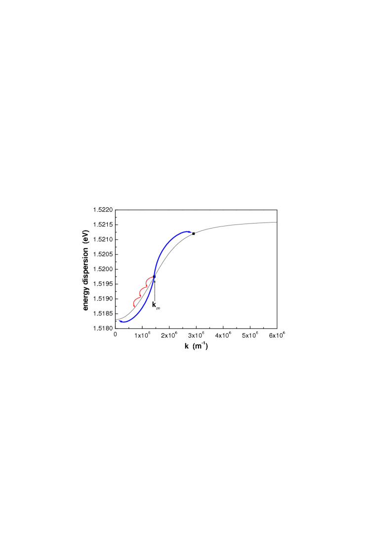
In order to perform numerical calculations, we need to discretize in ${\bf k}$-space. Although, thanks to confinement, cavity photons acquire a mass, it is about 4 order of magnitude smaller than the typical exciton mass, thus the polariton splitting results in a very steep energy dependence on the in-plane wave vector near ${\bf k}=0$ ($k=\omega\sin{\theta}/c$) (see Fig.  1). This very strong variation of the polariton effective mass with momentum makes difficult the numerical integration of the polariton PL rate-equations (IV). For example if PL originates from a pump beam set at the magic-angle (see Fig.  1) or beyond, a small temperature of $5$ K is sufficient to enable scattering processes towards states at quite higher $k$-vectors, thus it is necessary to include a computational window in k-space, significantly beyond ${\bf k}_{pump}$. Usually, in finite volume numerical calculations, the ${\bf k}$-space mesh is chosen uniform, but a dense grid suitable for the strong coupling region would result in a grid of prohibitively large number of points for (e.g. thermally activated) higher ${\bf k}$, on the other hand a mesh well-suited for polaritons at higher k-values would consist of so few points close to ${\bf k}=0$ to spoil the results gathered from the numerical code completely of their physical significance. Following Ref. Tassone Yam PRB 1999 we choose a uniformly spaced grid in energy which results in an adaptive ${\bf k}$-grid (in modulus), in addition, thanks to the rotating symmetry of the dispersion curve, we choose a uniformly distributed mesh in the angle $\theta$ so that ${\bf k}=(k,\theta)$. Unfortunately, even if this choice allows for a numerical integration of the polariton PL rate equations (IV), it provides an unbearable poor description of the parametric processes (V). The incoherent scattering events and the PL emission rates are strongly dependent on the energy of the involved polariton states. On the contrary parametric emission, being resonant when total momentum is conserved, depends strongly on both the zenithal $\theta$ and azimuthal $\phi$ angles which become poorly described by such adaptive mesh when the dispersion curve becomes less steep. Our DCTS-Langevin method enables the (computationally advantageous) decoupling of incoherent dynamics from parametric processes allowing us to make the proper choices for the two contributions whenever needed.

In particular, we seed the system at a specific ${\bf k}$ and first of all we calculate the pump-induced PL by means of Eq.  (IV). Because of the very steep dispersion curve and the large portion of ${\bf k}$-space to be taken into account, in the numerical solution we need to exploit the adaptive grid above mentioned. Afterwards we use this pump-induced PL, $\langle\hat{P}^{\dagger}_{\bf k}\hat{P}_{\bf k}\rangle_{\text{PL}}$, as a known input source in Eq.  (V) where it is largely more useful to discretize uniformly in ${\bf k}$.

We consider a SMC analogous to that of Refs. Savasta PRL2005 ; Langbein PRB2004 consisting of a $25$ nm $\text{Ga}\text{As}/\text{Al}_{0.3}\text{Ga}_{0.7}\text{As}$ single quantum well placed in the center of a $\lambda$ cavity with $\text{Al}\text{As}/$$\text{Al}_{0.15}\text{Ga}_{0.85}\text{As}$ Bragg reflectors. The lower polariton dispersion curve is shown in Fig.  1. The simulations are performed at $T=5\,\text{K}$ and the measured cavity linewidth is $\hbar\gamma_{c}=0.26\,\text{meV}$. The laser pump is modeled as a single Gaussian-shaped impulse of FWHM $\tau=1\,\text{ps}$ exciting a definite wave vector ${\bf k}_{p}$ and centered at $t=4\,\text{ps}$. We pump with co-circularly polarized light exciting polaritons with the same polarization, the laser intensities $I$ are chosen as multiple of $I_{0}$ corresponding to a photon flux of $21\,\mu\text{m}^{-2}$ per pulse. We observe that Ref. Langbein PRB2004 excites with a linearly polarized laser whose intensities $I^{L}$ are multiple of an $I^{L}_{0}$ corresponding to a photon flux of $21\,\mu\text{m}^{-2}$ per pulse too. In situations where the PSF and the MF terms dominate the nonlinear parametric interaction, there is no polarization mixing and two independent parametric processes take place, the first involving circularly polarized modes only and the second involving counter-circularly polarized modes. Thus for comparison with theory the effective density in those experiments is half the exciting density: $I=I^{L}/2$.

It has been theoretically shownPiermarocchi bottleneck , that it is quite difficult to populate the polaritons in the strong coupling region by means of phonon-scattering due to a bottleneck effect, similar to that found in the bulk. Let us consider a pump beam resonantly exciting polaritons at about the magic-angle. Relaxation by one-phonon scattering events is effective when the energy difference of the involved polaritons do not exceeds $1\,\text{meV}$. When polariton states within this energy window get populated, they can relax by emitting a phonon to lower energy levels or can emit radiatively. Owing to the reduced density of states of polaritons and to the increasing of their photon-component at lower energy, radiative emission largely exceeds phonon scattering, hence inhibiting the occupation of the lowest polariton states. Actually this effect is experimentally observed only very partially and under particular circumstancesTartakovskii PRB . This is mainly due to other more effective scattering mechanismsDi Carlo Kavokin PRB usually present in SMCs. For example the presence of free electrons in the system determines an efficient relaxation mechanism. Here we present results obtained including only phonon-scattering. Nevertheless the theoretical framework here developed can be extended to include quite naturally other enriching contributions that enhance non-radiative scattering and specifically relaxation to polaritons at the lowest k-vectorsDi Carlo Kavokin PRB . In order to avoid the resulting unrealistic low non-radiative scattering particularly evident at low excitation densities, we artificially double the acoustic-phonon scattering rates. However, acting this way, we obtain non-radiative relaxation rates that in the mean agree with experimental values.

We now present the results of numerical solutions of Eq.  (LABEL:PcrP_Langevin) taking into account self-stimulation but neglecting the less relevant pump-induced renormalization of polariton energies.

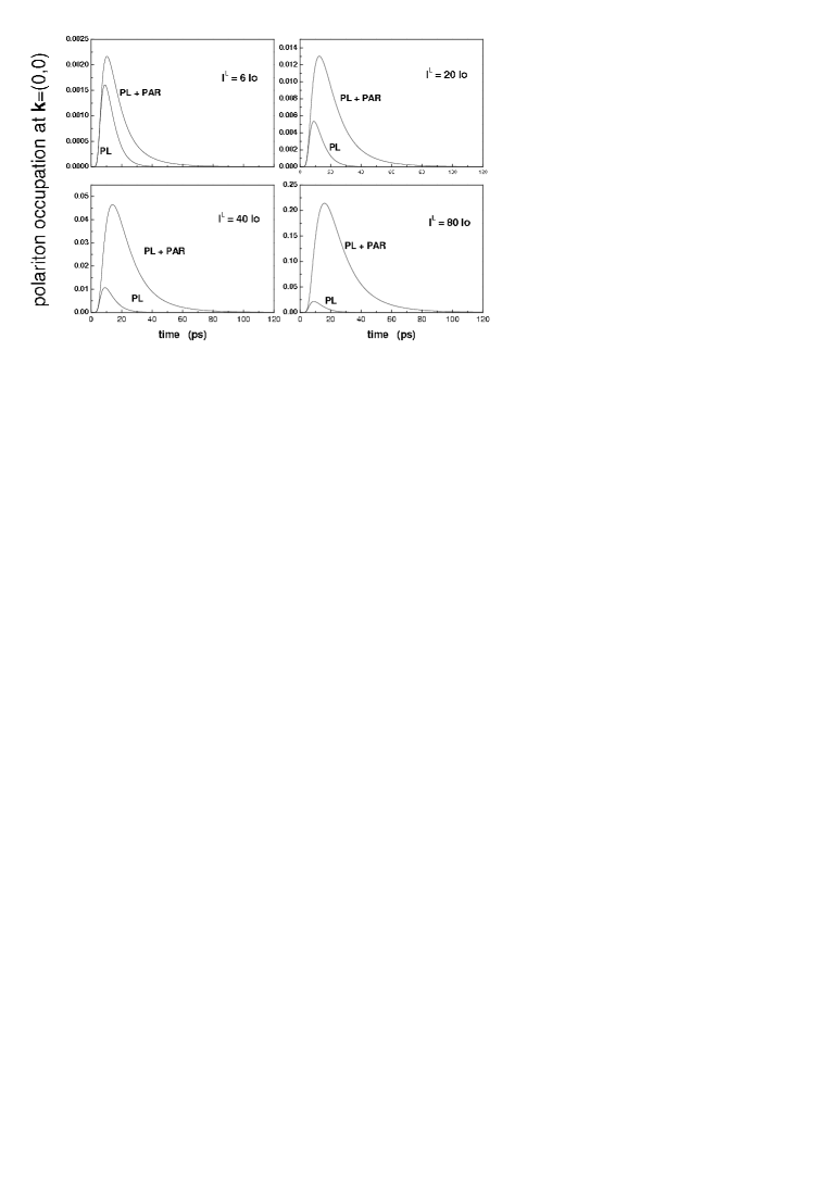
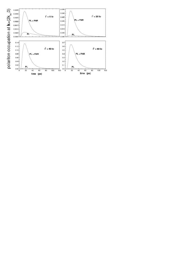
Figures  2 and 3 show the calculated time dependent polariton mode-occupation of a signal-idler pair at ${\bf k}=(0,0)$ and at ${\bf k}=(2\,k_{m},0)$, respectively, obtained for four different pump intensities in comparison with the time dependent pump-induced PL at the corresponding ${\bf k}$. The pump beam is sent at the magic angle Baumberg ($k_{m}\simeq 1.44\cdot 10^{6}\,\text{m}^{-1}$) which is close to the inflection point of the energy dispersion curve and is resonant with the polariton state at $k_{m}$. The magic angle is defined as the pump value needed for the eight-shaped curve of the resonant signal-idler pairs to intersect the minimum of the polariton dispersion curve. It is worth noting that the displayed results have no arbitrary units. We address realistic input excitations and we obtain quantitative outputs, indeed in Figs.  2 and 3 we show the calculated polariton occupation, i.e. the number of polaritons per mode. In our calculations no fitting parameter is needed, nor exploited (apart from the doubling of the phonon scattering rates). Moreover our results predict in good agreement with the experimental results of Ref.  Langbein PRB2004 the pump intensity at which parametric scattering, superseding the pump-PL, becomes visible. It is clear the different pump-induced PL dynamics of the mode-occupation at $k_{x}=2\,k_{m}$ (Fig.  3) with respect to that at the bottom of the dispersion curve of Fig.  2. Specifically a residual queue at high time values, due to the very low radiative decay of polaritons with k-vectors beyond the inflection point, can be observed. Furthermore we notice that already at moderate pump excitation intensities the parametric contribution dominates. It represents a clear evidence that we may device future practical experiments exploiting such a window where the detrimental pump-induced PL contribution is very low meanwhile we face a good amount of polaritons per mode. Indeed for photon-counting coincidence detections to become a good experimental mean of investigation we need a situation where accidental detector’s clicks are fairly absent and where the probability of states with more than one photon is low. Our results clearly show that there is a practical experimental window where we would address a situation where all these conditions would be well fulfilled.

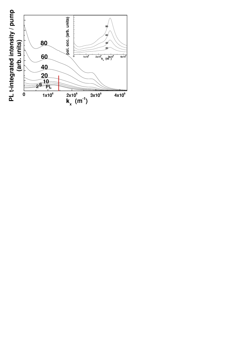
We now focus our attention on the positive part of the $k_{y}=0$ section at different pump powers. In Fig.  4 we observe the clear evidence of the build-up of the parametric emission taking over the pump-induced PL once the seed beam has become enough intense, in particular we can set a threshold around $I=10\,I_{0}$ ($I^{L}=20\,I_{0}$). As expected, the parametric process with the pump set at the magic angle enhances the specific signal-idler pair with the signal in ${k_{x}=0}$ and the idler in ${k_{x}=2k_{m}}$. We can clearly see from the figure that at pump intensities higher than the threshold the idler peak becomes more and more visible for increasing power in agreement of what shown in Ref. Baumberg and Ref.  Baumberg PRB(R) . However, at so high $k_{x}$ values the photon component is very small and even if the polariton idler occupation is very high (as the inset if Fig.  4 shows), the outgoing idler light is so weak to give some difficulties in real experimentsLangbein PRB2004 . Moreover we can notice that the parametric process removes the phonon bottleneck in the region close to ${\bf k}=0$. An analogous situation occurs also in Ref. Tartakovskii PRB , though with a different SMC, where it can be seen the bottleneck removal in ${\bf k}=0$ due to the parametric emission.

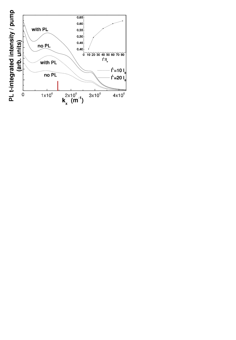
Fig.  5 shows the impact on the time integrated patterns of the calculated pump-induced PL. We consider, for different excitation intensities, the solutions of Eq.  (V) with and without the pump-induced PL occupations. As can be seen its inclusion does not result in an uniform noise background, but it seems to somewhat remember its incoherent nonuniform distribution (the one depicted in the corresponding curve, i.e. $\text{PL}_{\text{pump}}$, in Fig.  4). As can be clearly gathered from the figure, the pump-induced PL has a non negligible contribution in a region in ${\bf k}$-space resonant for the parametric processes. As a consequence at intermediate excitation intensities it adds up to the parametric part reaching a contribution even comparable to the peak of emission set in ${\bf k}=0^{+}$. Only beyond the above mentioned threshold the parametric emission is able to take over pump-induced PL and results in the great emission in the bottom of the dispersion curve of Ref. Baumberg . These results clearly show that PL emission does not become negligible at quite high excitation densities, but, being amplified by the parametric process, determines a redistribution of polariton emission displaying qualitative differences with respect to calculations neglecting PL. An interesting question regarding these phenomena could be related to the impact in the global spontaneous emission of the two contributions in Eq.  (V), namely that of the homogeneous part $|c_{2}(0,t)|^{2}$ and the one originating from noise operators in the time integral in the last line. In the inset of Fig.  5 we have depicted the ratio of the homogenous solution with the global emission at ${\bf k}=0^{+}$, calculated without $\langle\hat{P}^{\dagger}_{\bf k}\hat{P}_{\bf k}\rangle_{\text{PL}}$. Rather surprisingly when increasing the pump intensity the two contributions (homogeneous and particular) continue to have comparable weights, hence for a proper description of the spontaneous parametric emission they must be both included.

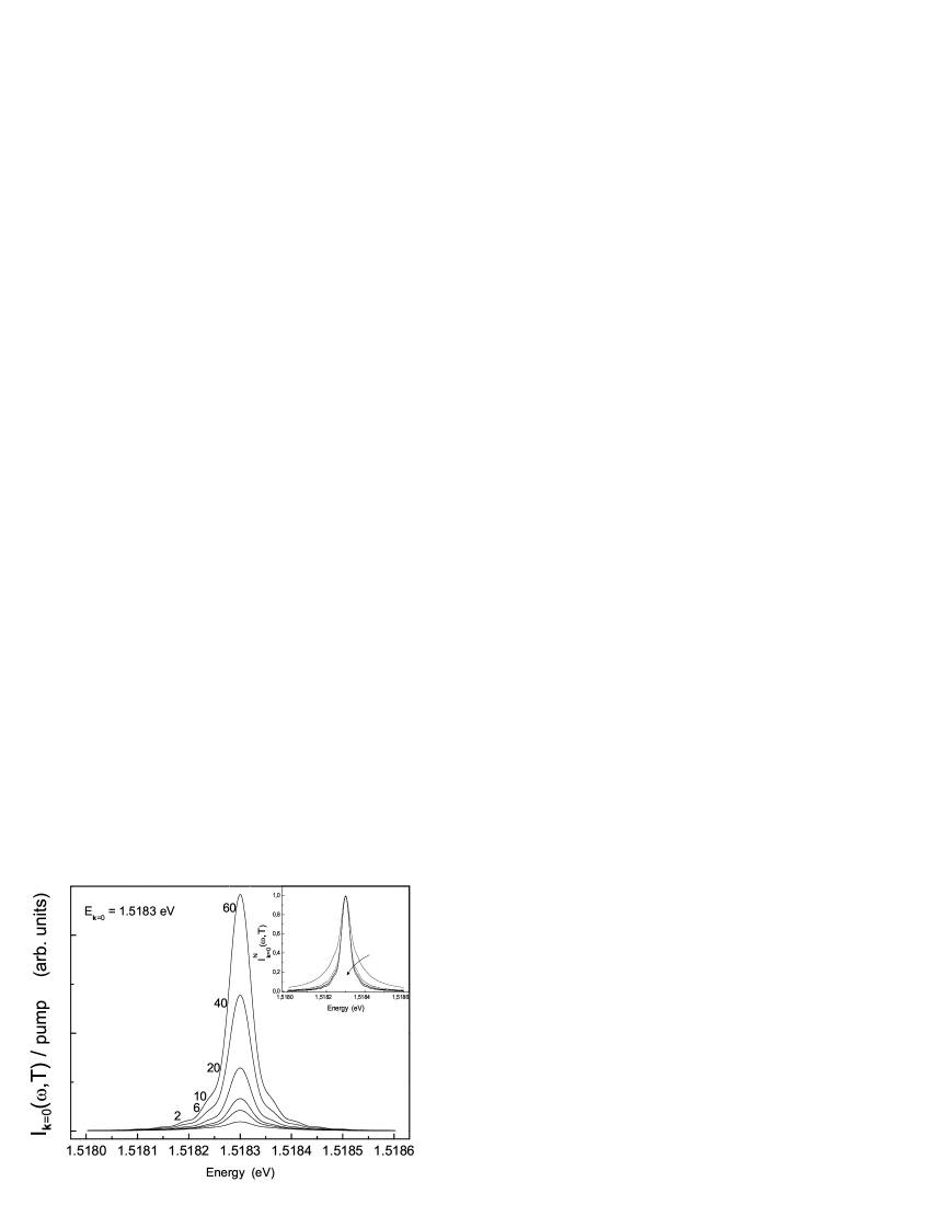
The calculated time-integrated spectra of the outgoing light at ${\bf k}=(0,0)$ obtained at six different pump intensities for an excitation at the magic angle $k_{m}$ are shown in Fig.  4. It can be easily noticed a threshold around $I^{L}=20\,I_{0}$ in perfect agreement with the results in Fig.  4 and with Ref.  Langbein PRB2004 . For intensities lower than the threshold, the signal in ${k_{x}=0}$ (with the corresponding idler in ${k_{x}=2k_{m}}$) shows a quite large nearly Lorentian shape. As soon as the threshold is passed over, the spectrum starts to increase super-linearly with some spurious queues due to (calculated) asymmetric signal/idler damping values. Noticeably the spectra show an evident linewidth narrowing for increasing pump intensities witnessing the parametric emission build-up. For the sake of presentation in the inset we also present some normalized spectra which give immediate evidence of the build-up of a narrow linewidth beyond the mentioned threshold.

VII Summary and conclusions

Based on a DCTS theoretical framework for interacting polaritons (see Sect. 2), we have presented a general theoretical approach for the realistic investigation of polariton quantum correlations in the presence of coherent and incoherent interaction processes. The proposed theoretical framework combines the dynamics controlled truncation scheme with the nonequilibrium quantum Langevin approach to open systems. It provides an easy recipe to calculate multi-time correlation functions which are key-quantities in quantum optics, but as shown here even for single-time quantities it provides a natural and advantageous decoupling of incoherent dynamics from parametric processes. We have elaborated equations whose structure is analogous to those one obtains by means of bosonization Ciuti SST . However, thanks to the DCTS approach we have been able to obtain microscopically nonlinear coefficients with great accuracy. In particular in Ref. Ciuti SST the nonlinear coupling coefficient contains additional terms due to phase space filling providing an interaction strength larger of about a factor 3. We believe that the difference is due to the way how the Bosonization procedure has been adopted. As a first application of the proposed theoretical scheme, we have analyzed the build-up of polariton parametric emission in semiconductor microcavities including the influence of noise originating from phonon induced scattering. Our numerical results clearly show the importance of a proper microscopic analysis able to account for parametric emission and pump-induced PL on an equal footing in order to make quantitative comparison and propose future experiments, seeking and limiting all the unwanted detrimental contributions. Specifically, we have shown that already at moderate pump excitation intensities there are clear evidence that we may device future practical experiments exploiting existing situations where the detrimental pump-induced PL contribution is very low meanwhile we face a good amount of polaritons per mode. It represents an exciting and promising possibility for future coincidence experiments even in photon-counting regimes, vital for investigating nonclassical properties of the emitted light.

*

Appendix A The interactions with reservoirs

A quasi-two-dimensional exciton state with total in-plane center of mass (CM) wave vector ${\bf k}$ may be represented as Takagahara

$$\mid\lambda,{\bf k}\rangle\!\!=\!\!\frac{v_{0}}{\sqrt{S}}\!\!\sum_{\bf r_{e},r_{h}}\!\!e^{i\bf k\cdot R^{\|}}F_{\lambda}({\bf r^{\|}_{e}-\bf r^{\|}_{h}},z_{e},z_{h})a^{\dagger}_{c,{\bf r_{e}}}a_{v,{\bf r_{h}}}\!\!\mid 0\rangle\,,$$ (70)

where $v_{0}$ and $S$ are the volume of the unit cell and the in-plane quantization surface, whereas $a^{\dagger}_{c/v,{\bf r}}(a_{c/v,{\bf r}})$ are creation (annihilation) operator of the conduction- or valence- band electron in the Wannier representation. ${\bf r}_{e/h}=({\bf r}^{\|}_{e/h},z_{e/h})$ are to be considered coordinates of the direct lattice, $\mid\!\!0\rangle$ is the crystal ground state and ${\bf R}$ the exciton center of mass coordinate ${\bf R}=(m_{e}{\bf r}_{e}+m_{h}{\bf r}_{h})/(m_{e}+m_{h})$ with $m_{e}$ and $m_{h}$ the effective electron and hole masses. The Wannier envelope function $F_{\lambda}$ is normalized so that the integral over the whole quantization volume $(V\!\!=S\!\!\cdot\!\!L)$ of its square modulus is equal to 1. The lattice properties of GaAs-AlAs QW structures are in close proximity, thus the acoustic-phonons which interact with the quasi-two-dimensional exciton can be considered to have three-dimensional character. The electron-phonon interaction Hamiltonian resulting from the deformation potential coupling, can be written as

$$H^{DF}_{e-ph}=\sum_{\bf k,q} \left(\frac{\hbar|{\bf q}|}{2\rho uV}\right)^{1/2}\left(D_{c}a^{\dagger}_{c,{\bf k+q}}a_{c,{\bf k}}+D_{v}a^{\dagger}_{v,{\bf k+q}}a_{v,{\bf k}}\right)\left(b_{\bf q}+b^{\dagger}_{-\bf q}\right)\,.$$ (71)

Here $a^{\dagger}_{c/v,{\bf k}},a_{c/v,{\bf k}}$ are creation and destruction operator of the conduction- valence- band electron in Bloch representation. Transforming from the Wannier to the Bloch representation, we shall project (71) into the excitonic bases. Moreover, since we are interested in the 1S exciton sector $\lambda=(n,\sigma)$ only

$$F_{1S}=W_{1S}({\bf r^{\|}_{e}-\bf r^{\|}_{h}})\chi_{e}(z_{e})\chi_{h}(z_{h})$$

$$W_{1S}(\rho)=\sqrt{2/(\pi a^{2}_{\text{x}})}\exp(-\rho/a^{2}_{\text{x}})\,.$$ (72)

It yields

$$H^{DF}_{exc-ph}= \sum_{{\bf k,k^{\prime}},q_{z}}t^{{\bf k}^{\prime},q_{z}}_{{\bf k}}\mid 1S\,{\bf k^{\prime}}\rangle\langle 1S\,{\bf k}\mid\left(b_{({\bf k^{\prime}-k},q_{z})}+b^{\dagger}_{-({\bf k^{\prime}-k},q_{z})}\right)\,,$$ (73)

here

$$t^{{\bf k}^{\prime}\!,q_{z}}_{{\bf k}}\!\!\! = \!\!\left(\frac{\hbar\sqrt{|{\bf k^{\prime}-k}|+q^{2}_{z}}}{2\rho uV}\right)^{1/2}\left(D_{c}I^{\bot}_{e}(q_{z})I^{\|}_{e}({\bf k^{\prime}-k})-D_{v}I^{\bot}_{h}(q_{z})I^{\|}_{h}({\bf k^{\prime}-k})\right)\,,$$ (74)

being $I^{\bot}$ and $I^{\|}$ overlap integrals given in Eq.  (IV).

We treat the cavity field in the quasi-mode approximation, that is to say we shall quantize the field as the mirror were perfect and subsequently we shall couple the cavity with a reservoir of a continuum of external modes. The coupling of the electron system and the cavity modes is given in the usual rotating wave approximation

$$H_{qm}\!\!=i\hbar\sum_{\bf k}\!\!\int\!\!\!d\omega g_{\bf k}(\omega)a^{{\dagger}}_{\bf k}E^{(-)}_{\bf k}(\omega,t)+H.c.\,,$$ (75)

In passing form the air to the SMC, we change from a 3D to a 2D quantization, it means that in the coupling once either $({\bf k},k_{z})$ or $({\bf k},\omega)$ is chosen the third follows consistently. We have chosen the latter for simplicity in dealing with the Markov machinery. In the Hamiltonian $g_{\bf k}(\omega)$ is the coupling coefficient, a sort of optical matrix element, $E^{(-)}_{\bf k}(\omega,t)$ and $E^{(+)}_{\bf k}(\omega,t)$ are the two propagating normal modes of the external light. Modeling the loss through the cavity mirrors within the quasi-mode picture means we are dealing with an ensemble of external modes, generally without a particular phase relation among themselves. An input light beam impinging on one of the two cavity mirrors is an external field as well and it must belong to the family of modes of the corresponding side (i.e. left or right). It will be nothing but the non zero expectation value of the (coherent) photon operator giving a non zero contribution on the $1^{\text{st}}$ perturbative order. All the other incoherent bath modes will have their proper contribution in the $2^{\text{nd}}$ order calculations.

It is worth noting that the treatment of the cavity losses as a scattering interaction is a result of the form chosen of the effective quasi-mode Hamiltonian. However, even if a model Hamiltonian, the quasi-mode description has given a lot of evidence as an accurate modeling tool and it is widely used in the literature. Let us call $R$ the quasi-mode reservoir Hamiltonian. It can be shown that the first order (coherent) dynamics for a generic operator $\hat{O}$ under the influence of the coherent part of the quasi-mode ensemble reads, (see Eq.  (75))

$$i\hbar\frac{d\langle\hat{O}\rangle}{dt}{\left|\right._{H_{qm}}}=i\hbar\sum_{{\bf k}}\sum_{p}g_{p}\left<\right.E^{(-)}_{p}(\Omega_{p},t)\left.\right>_{R}\left<\right.[\hat{O},a^{\dagger}_{\bf k}]\left.\right>+H.c.\,,$$ (76)

where $g_{\bf k}(\omega)$ is the coupling coefficient, $E^{(-)}_{\bf k}(\omega,t)$ is the propagating normal mode of the external light and $\sum_{p}g_{p}\left<\right.E^{(-)}_{p}(\Omega_{p},t)\left.\right>_{R}$ is the superposition of all the possible coherent pump feeds.

An interesting situation occurs within the assumption of a flat quasi-mode spectrum, an approximation almost universally made in quantum optics Collet Gardiner PRA 1985 . It makes Eq.  (58) independent of the frequency:

$$\gamma^{(c)}_{\alpha,{\bf k}}=\sum_{i=l,r}\frac{2\pi}{\hbar}|C_{\alpha,{\bf k}}|^{2}\hbar|g_{i,{\bf k}}|^{2}=|C_{\alpha,{\bf k}}|^{2}\sum_{i=l,r}\gamma^{(m)}_{i,{\bf k}}\,,$$ (77)

where $\gamma^{(m)}_{i,{\bf k}}$ is the (i-side) damping of the cavity without the quantum well.

Thus

$$\sum_{i=l,r}\gamma^{(m)}_{i,{\bf k}}=2\pi\sum_{i=l,r}|g_{i,{\bf k}}|^{2}\,,$$ (78)

there are two situations:

• equal damping: $\gamma^{(m)}_{{l,\bf k}}=\gamma^{(m)}_{{r,\bf k}}$, we can define the transmission coefficient of the i-side

  $$|g_{i,{\bf k}}|^{2}=\frac{\gamma^{(m)}_{{i,\bf k}}}{2\pi}\doteq t^{2}_{c,i}$$ (79)

• we know the ratio:

  $$\left\{\begin{array}[]{ll}R=\frac{\gamma^{(m)}_{{r,\bf k}}}{\gamma^{(m)}_{{l,\bf k}}}\\ \gamma^{(m)}_{{\text{tot},\bf k}}=\gamma^{(m)}_{{r,\bf k}}+\gamma^{(m)}_{{l,\bf k}}\\ \end{array}\right.\Rightarrow\left\{\begin{array}[]{ll}\gamma^{(m)}_{{l,\bf k}}=\frac{1}{1+R}\gamma^{(m)}_{{\text{tot},\bf k}}\\ \gamma^{(m)}_{{r,\bf k}}=\frac{R}{1+R}\gamma^{(m)}_{{\text{tot},\bf k}}\\ \end{array}\right.$$

and the transmission coefficients follow.

In the light of the definition of $t^{2}_{c,i}$, it becomes evident that the semiclassical coherent input feed could also be modeled from the beginning with an effective Hamiltonian:

$$H_{p}=i\hbar\sum_{{\bf k}}({E}^{(-)}_{{\bf k}}\hat{a}^{\dagger}_{{\bf k}}-{E}^{(+)}_{{\bf k}}\hat{a}_{{\bf k}})\,,$$ (80)

where (the $\mathbb{C}-$numbers) ${E}^{(\pm)}_{{\bf k}}=\sum_{p}t_{c,p}\left<\right.E^{(\pm)}_{p}(\Omega_{p},t)\left.\right>_{R}$ represent the incoming coherent input beams Savasta PRL96 .

Figure 1: (color online) Energy dispersion of the lowest polariton branch for the structure of Ref.  Langbein PRB2004 consisting of a $25$ nm $\text{Ga}\text{As}/\text{Al}_{0.3}\text{Ga}_{0.7}\text{As}$ single quantum well placed in the center of a $\lambda$ cavity with $\text{Al}\text{As}/$$\text{Al}_{0.15}\text{Ga}_{0.85}\text{As}$ Bragg reflectors. The pump at the magic angle and its parametric scattering (blue curve) are schematically depicted. The latter scatters two pump polaritons in a signal-idler couple at ${\bf k}=0$ and ${\bf k}=2{\bf k}_{m}$. The red curve symbolizes incoherent pump scattering at $\text{T}=0\,\text{K}$, e.g. due to acoustic phonon interaction. Because of the very steep dispersion curve in the strong coupling region due to strong coupling, for a pump beam set at the magic angle or beyond, even a small temperature of $5$ K is sufficient to enable scattering processes towards states at quite higher $k$-vectors, thus it becomes necessary to include a computational window in k-space, significantly beyond ${\bf k}_{pump}$ making difficult numerical simulations.

Figure 2: Calculated time dependent polariton mode-occupation at ${\bf k}=(0,0)$ obtained at four different pump intensities in comparison with the time dependent pump-induced PL at the corresponding ${\bf k}$. The laser pump is modeled as a single Gaussian-shaped impulse of FWHM $\tau=1\,\text{ps}$ exciting a definite wave vector ${\bf k}_{p}=(k_{m},0)$ and centered at $t=4\,\text{ps}$. The calculated values are in good quantitative agreement with the measured value of Ref.Langbein PRB2004 , with no fitting parameter needed nor exploited.

Figure 3: Calculated time dependent polariton mode-occupation at ${\bf k}=(2\,k_{m},0)$. It has been obtained under the same condition as Fig.  2. It is clear the different pump-induced PL dynamics with respect to Fig.  2, specifically a residual queue at high time values.

Figure 4: Time-integrated outgoing photon emission intensity. The pump is set at ${\bf k}_{p}=(k_{m},0)$. It is clear the evidence of the build-up of the parametric emission taking over the pump-induced PL once the seed beam becomes higher than the threshold around $I^{L}=20\,I_{0}$. Moreover the parametric process removes the phonon bottleneck in the region closed to ${\bf k}=0$. As expected the specific signal-idler parametric scattering with the signal in ${k_{x}=0}$ and the idler in ${k_{x}=2k_{m}}$ is favourite and at higher pump intensities dominates the light emission. The polariton idler occupations for some pump values are depicted in the inset. Although polariton occupation at ${k_{x}=2k_{m}}$ is so high, its photonic component is very small resulting in a very weak outgoing light beam.

Figure 5: The impact on the time integrated patterns of the calculated pump-induced PL for different excitation intensities is shown (the pump is set in ${\bf k}_{p}=(k_{m},0)$). Here the solutions of Eq.  (V) with and without the pump-induced PL occupations are depicted. On the contrary to what implicitly considered in previous phenomenological theories it results in a non-uniform noise background and hence its momentum distribution has to be included for a realistic microscopic calculation of the emission patterns. Moreover it is non-negligible in a region in ${\bf k}$-space resonant for the parametric processes and hence at intermediate excitation intensities it adds up to the parametric part reaching a contribution even comparable to the peak of emission set in ${\bf k}=0^{+}$ up to the threshold around $I^{L}=20\,I_{0}$. In the inset the ratio of the homogenous solution with the global emission at ${\bf k}=0^{+}$ (both calculated without $\langle\hat{P}^{\dagger}_{\bf k}\hat{P}_{\bf k}\rangle_{\text{PL}}$) is depicted. For increasing pump intensities the two contributions (homogeneous and particular) in Eq.  (V) still display comparable contributions, hence for a proper description of the spontaneous parametric emission they must be both included.

Figure 6: Calculated time-integrated spectrum of the outgoing light at ${\bf k}=(0,0)$ normalized with respect to the pump seed obtained at six different pump intensities for an excitation at the magic angle $k_{m}$. It can be easily noticed a threshold around $I^{L}=20\,I_{0}$ in perfect agreement with the results in Fig.  4 and with Ref.  Langbein PRB2004 . For intensities lower than the threshold, the signal in ${k_{x}=0}$ (with the corresponding idler in ${k_{x}=2k_{m}}$) shows a quite large nearly Lorentian shape, as soon as the threshold is passed over the spectrum start to increase super-linearly meanwhile the linewidth decreases witnessing the parametric emission build-up. In the inset the normalized spectra at increasing pump powers (indicated by the arrow direction) are depicted evidencing even better the linewidth narrowing. We notice also some spurious queues due to (calculated) asymmetric signal/idler damping values.

References

- (1) M. A. Nielsen and I. L. Chuang, Quantum Computation and Quantum Information (Cambridge University Press, Cambridge, 2000).
- (2) V. M. Axt and T. Kuhn, Rep. Progr. Phys. 67 433-512 (2004).
- (3) B. Hönerlage, A. Bivas, and Vu Duy Phach, Phys. Rev. Lett. 41, 49 (1978).
- (4) R. M. Stevenson et al., Phys. Rev. Lett. 85, 3680 (2000).
- (5) S. Savasta and R. Girlanda, Phys. Rev. Lett. 77 4736 (1996).
- (6) K. Victor, V. M. Axt, A. Stahl, Phys. Rev. B 51, 14164 (1995).
- (7) S. Savasta and R. Girlanda, Phys. Rev. B 59, 15409 (1999).
- (8) S. Savasta, G. Martino, and R. Girlanda, Solid State Communication, 111 495 (1999).
- (9) S. Savasta, O. Di Stefano, and R. Girlanda, Phys. Rev. Lett 90, 096403 (2003).
- (10) C. Weisbuch et al., Phys. Rev. Lett. 69, 3314 (1992); R. Houdre et al., Phys. Rev. Lett. 85, 2793 (2000).
- (11) J. Erland et al., Phys. Rev. Lett. 86, 5791 (2001).
- (12) W. Langbein, Phys. Rev. B 70, 205301 (2004).
- (13) P. Schwendimann, C. Ciuti, and A. Quattropani, Phys. Rev. B 68, 165324 (2003)
- (14) S. Kundermann, M. Saba, C. Ciuti, T. Guillet, U. Oesterle, J. L. Staehli, and B. Deveaud, Phys. Rev. Lett. 91, 107402 (2003).
- (15) C. Ciuti, Phys. Rev. B 69, 245304 (2004).
- (16) S. Savasta, O. D. Stefano, V. Savona, and W. Langbein, Phys. Rev. Lett. 94, 246401 (2005).
- (17) K. Edamatsu, G. Oohata, R. Shimizu, and T. Itoh, Nature 431, 167-170 (2004).
- (18) C. Diederichs, J. Tignon, G. Dasbach, C. Ciuti, A. Lema tre, J. Bloch, Ph. Roussignol and C. Delalande, Nature 440, 904 (2006).
- (19) C. Ciuti, P. Schwendimann, and A. Quattropani, Phys. Rev. B 63, 041303 (2001).
- (20) B. Krummheuer, V. M. Axt, T. Kuhn, I. D’Amico, and F. Rossi, Phys. Rev. B 71, 235329 (2005).
- (21) C. Ciuti, P. Schwendimann, B. Deveaud, A. Quattropani, Phys. Rev. B 62, R4825 (2000).
- (22) S. Portolan, S. Savasta, O. Di Stefano, F. Rossi, and R. Girlanda, arXiv:0706.2241v2 [cond-mat.mes-hall], submitted.
- (23) Th. Österich, K. Schönhammer, and L. J. Sham, Phys. Rev. Lett. 74, 4698 (1995), Phys. Rev. B 58, 12920 (1998).
- (24) C. Ciuti, P. Schwendimann, A. Quattropani, Semicond. Sci. Technol. 18, S279 (2003).
- (25) See e.g. D. F. Walls and G. J. Milburn Quantum Optics Springer-Verlag (Berlin-Heidelberg) 1994.
- (26) L. Mandel, E. Wolf Optical Coherence and Quantum Optics (Cambridge University Press) 1995.
- (27) G. W. Ford, J. T. Lewis, and R. F. O Connell, Phys. Rev. A 37, 4419 (1988).
- (28) M. Lax, Phys. Rev., 145 110 (1966).
- (29) S. Savasta, O. Di Stefano, and R. Girlanda, Phys. Rev. B 64, 073306 (2001).
- (30) F. Tassone,C. Piermarocchi, V. Savona, A. Quattropani, P. Schwendimann, Phys. Rev B. 56, 7554 (1997).
- (31) J. H. Eberly and K. Wódkiewicz, J. Opt. Soc. Am. 67, 1252 (1977).
- (32) J. D. Cresser, Phys. Rep 94, 47 (1983).
- (33) C. W. Gardiner and M. J. Collett, Phys. Rev. A 31, 3761 (1985).
- (34) B. Renaud, R.M. Whitley and C.R. Stroud Jr., J. Phys. B 10, 19 (1977).
- (35) F. Tassona, Y. Yamamoto, Phys. Rev B 59, 10830 (1999).
- (36) A. I. Tartakovskii et al., Phys. Rev. B 62, R2283 (2000).
- (37) G. Malpuech, A. Kavokin, A. Di Carlo, and J. J. Baumberg, Phys. Rev. B 65, 153310 (2002).
- (38) P.G. Savvidis et. al., Phys. Rev. B 62, R13278 (2000).
- (39) T. Takagahara, Phys. Rev. B, 31, 6552 (1985).