Predicting spinor condensate dynamics from simple principles

Abstract

We study the spin dynamics of quasi-one-dimensional $F=1$ condensates both at zero and finite temperatures for arbitrary initial spin configurations. The rich dynamical evolution exhibited by these non-linear systems is explained by surprisingly simple principles: minimization of energy at zero temperature, and maximization of entropy at high temperature. Our analytical results for the homogeneous case are corroborated by numerical simulations for confined condensates in a wide variety of initial conditions. These predictions compare qualitatively well with recent experimental observations and can, therefore, serve as a guidance for on-going experiments.

Spinor condensates realized by optically trapped ultracold atoms in a hyperfine Zeeman manifold allow to address a broad scope of problems, which are related to magnetic ordering. These include quantum phase transitions, exotic topological defects and spin domains either within a mean-field regime or within the strongly-correlated one lewen07 . Already in the mean-field regime the dynamics of spinor condensates shows some intriguing features, with an apparent randomness regarding the evolution from a given initial state towards a steady state, accompanied by formation of spin domains. Even for the simplest case of an $F=1$ spinor condensate, the interplay between spin-spin interactions, non-linear terms and temperature effects rends the analysis of the dynamics rather complex. Previous studies of the spinor dynamics show that, at early stages of the evolution, there is a coherent population transfer between the different hyperfine coupled sublevels Mur06 ; Pu99 . Inclusion of temperature ($T$) not only smears out the population transfer Mur06 , but also leads to a different distribution of population among the different hyperfine levels.

In this contribution we analyze the dynamics of spinor $F=1$ condensates both at zero and finite $T$ from a new perspective. As we shall show, the complex dynamics displayed by these systems can be understood in terms of oscillations in phase space around a steady state. The configuration of this state can be approximately determined by analyzing the trajectories of constant energy in the homogeneous case. To a good approximation, the populations that characterize this state are rather close to those that minimize the energy associated to spin-spin interactions for a given magnetization. In contrast, at finite $T$, the system is able to exchange energy with the thermal clouds. At large enough temperature, the populations of the steady state can be simply determined by maximizing the entropy of the homogeneous condensate. This leads to a different long-time configuration of the populations than the one attained starting from the same initial conditions at $T=0$. Our claims are supported by analytical results for an homogeneous condensate and by numerical investigations for trapped condensates. They provide a good qualitative agreement with recent experimental data on the dynamics of spinor condensates nature ; Chang04 . Furthermore, our results can be straightforwardly used to analyze and predict experimental outcomes.

In the mean-field approach, the spinor condensate is described by a vector order parameter $\Psi$ whose components $\psi_{m}$ correspond to the order parameter of each magnetic sublevel $|F=1,m\rangle$ with $m=1,0,-1$. In absence of an external magnetic field and at $T=0$, the properties of the condensate are determined by the spin-dependent energy functional Mur06 ; Ho98 ; machida :

$${\cal E}=\, \int d^{3}r\left\{\psi^{*}_{m}\left(-\frac{\hbar^{2}}{2M}{\bm{\nabla}}^{2}+V_{ext}\right)\psi_{m}\right.$$

$$+\left.\frac{c_{0}}{2}\psi^{*}_{m}\psi^{*}_{j}\psi_{j}\psi_{m}+\frac{c_{2}}{2}\psi^{*}_{m}\psi^{*}_{j}{\bf F}_{mk}\cdot{\bf F}_{jl}\psi_{l}\psi_{k}\right\},$$ (1)

where repeated indices are assumed to be summed. The trapping potential is taken to be harmonic, axially-symmetric and spin independent. The coefficients $c_{0}$ and $c_{2}$ describe the spin-independent and the spin-dependent contributions of the binary elastic collisions of two identical spin-1 bosons. They are expressed in terms of the $s$-wave scattering lengths $a_{f}$ of the combined symmetric channels of total spin $f=0,2$ as $c_{0}=4\pi\hbar^{2}(a_{0}+2a_{2})/(3M)$ and $c_{2}=4\pi\hbar^{2}(a_{2}-a_{0})/(3M)$, where $M$ is the atomic mass. ${\bf F}$ are the spin-1 matrices Ho98 ; machida . In this Letter, we focus on ⁸⁷Rb spinor condensates nature ; Chang04 ; exper ; Higbie05 , which have ferromagnetic character ($c_{2}<0$).

According to $i\hbar\partial\psi_{m}/\partial t=\delta{\cal E}/\delta\psi_{m}^{*}$, a set of coupled dynamical equations for the spin components are obtained:

$$i\hbar\,\partial\psi_{\pm 1}/\partial t=\, [{\cal H}_{s}+c_{2}(n_{\pm 1}+n_{0}-n_{\mp 1})]\,\psi_{\pm 1}$$

$$+c_{2}\,\psi_{0}^{2}\psi^{*}_{\mp 1}\,,$$ (2a)

$$i\hbar\,\partial\psi_{0}/\partial t=\, [{\cal H}_{s}+c_{2}(n_{1}+n_{-1})]\,\psi_{0}$$

$$+2c_{2}\psi_{1}\psi_{0}^{*}\psi_{-1}\,,$$ (2b)

with ${\cal H}_{s}=-\hbar^{2}/(2M)\,{\bm{\nabla}}^{2}+V_{ext}+c_{0}n$ being the spin-independent part of the Hamiltonian. The density of the $m$-th component is given by $|\psi_{m}({\bf r})|^{2}$, while $n({\bf r})=\sum_{m}|\psi_{m}({\bf r})|^{2}$ is the total density normalized to the total number of atoms $N$. The population of each hyperfine state is $N_{m}=\int d{\bf r}|\psi_{m}({\bf r})|^{2}$. Defining the relative populations $\lambda_{m}=N_{m}/N$, the magnetization of the system is ${\cal M}=\lambda_{1}-\lambda_{-1}$. The total number of atoms and the magnetization are both conserved quantities Mur06 . Then, the conditions $\lambda_{1}+\lambda_{0}+\lambda_{-1}=1$ and ${\cal M}=\lambda_{1}-\lambda_{-1}$, together with the positiveness of $\lambda_{m}$, restrict the allowed configurations of the system in the $(\lambda_{0},{\cal M})$ phase space to the region below the dotted line in Fig. 1.

To understand the physics governing the spin dynamics, it is instructive to analyze first the homogeneous system at $T=0$. Translational invariance leads to the following ansatz: $\psi_{m}={\sqrt{n}}{\sqrt{\lambda_{m}}}\,e^{i\theta_{m}}$. Notice that, since the system is homogeneous, the value of $n$ is not relevant to determine the relative populations that minimize the energy. Thus, the only relevant contributions to the energy are those associated to $c_{2}$:

$$E_{c2}(\lambda_{0},\cal{M},\theta)=\; c_{2}n^{2}\big{[}\lambda_{0}(1-\lambda_{0})+{\cal M}^{2}/2$$

$$+\lambda_{0}{\sqrt{(1-\lambda_{0})^{2}-{\cal M}^{2}}}\,\cos\theta\big{]}\,,$$ (3)

where $\theta=2\theta_{0}-\theta_{1}-\theta_{-1}$. For a given value of ${\cal M}$, the ground state configuration is obtained by minimizing Eq. (3) with respect to $\lambda_{0}$ and $\theta$. For ferromagnetic systems, this yields $\theta=0$ and

$$\lambda_{0}^{eq}=\frac{1}{2}(1-{\cal M}^{2})\,,$$ (4)

which defines the solid line drawn in Fig. 1. For instance, in the symmetric case (${\cal M}=0$) the minimization leads to a ground state with $\lambda_{0}=0.5$ and $\theta=0$.

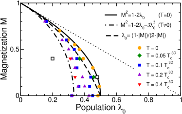
Figure 1: (color online) Equilibrium configurations in the $\lambda_{0}-{\cal M}$ plane for the homogeneous condensate at $T=0$ [solid line, Eq. (4)] and at large $T$ [dot-dashed line, Eq. (5)]. The dashed line in between indicates $\lambda_{0}^{min}$, the geometrical center of the closed orbit with the same magnetization, while the dotted line bounds the region of physically allowed values for $(\lambda_{0},{\cal M})$. Full symbols stand for the time averages of $\lambda_{0}(t)$ calculated from the numerical time evolution for different initial configurations at zero and finite $T$ for the inhomogeneous system; open squares indicate the initial conditions for the simulations at ${\cal M}=0.2,0.4$ respectively. Due to the symmetry of the equations, it suffices to present the results for positive magnetizations.

We study now the dynamical evolution of the homogeneous system by solving numerically the set of Eqs. (2), after removal of the terms $-\hbar^{2}/(2M)\,{\bm{\nabla}}^{2}+V_{ext}$. We consider three independent phases $\theta_{m}$ in the time evolution, although the energy depends only on the relative phase $\theta$ [Eq. (3)]. As expected, we find that starting from an equilibrium configuration (e.g. $\lambda_{0}=0.5$ and $\theta=0$ for ${\cal M}=0$) there is no evolution at all. However, if the initial configuration does not correspond to the equilibrium state, then the system evolves exchanging populations between spin components, but conserving energy and magnetization.

Therefore, in the homogeneous system the dynamical evolution of the spin populations is characterized by trajectories of constant energy and magnetization in the $\lambda_{0}-\theta$ plane, which are defined by the starting values of ${\cal M},\lambda_{0}$ and $\theta$. In most cases, i.e. if the initial conditions are not very far from the equilibrium configuration, defined by $\lambda_{0}^{eq}$ and $\theta=0$, the trajectories in the $\lambda_{0}-\theta$ plane are closed orbits (see also You12005 ). Then, the evolution of the populations –in particular of $\lambda_{0}$– shows up as oscillations of a well defined frequency, around the geometrical center of the orbit. An analysis of the orbits defined by Eq. (3), shows that these centers lie always between $\lambda_{0}^{eq}$ and $\lambda_{0}^{min}=(1-|{\cal M}|)/(2-|{\cal M}|)$, represented by the dashed curve in Fig. 1. With this information in mind we move now to the confined systems.

To this aim, we solve the equations of motion for 20000 atoms of ⁸⁷Rb, in a highly elongated trap $\omega_{\perp}=2\pi\times 891$ Hz and $\omega_{z}=2\pi\times 21$ Hz, i.e. $\omega_{\perp}\gg\omega_{z}$, so that Eqs. (2) become quasi-one-dimensional. The corresponding scattering lengths are $a_{0}=101.8a_{B}$ and $a_{2}=100.4a_{B}$, and the coupling constants $c_{0}$ and $c_{2}$ are accordingly rescaled by a factor $1/(2\pi a_{\perp}^{2})$, being $a_{\perp}=\sqrt{\hbar/m\omega_{\perp}}$ the transverse oscillator length  foot1 . The validity of this approximation for the case of a spin-1 atomic condensate has been proved for a very wide range of conditions in Ref. You12005 . We take as initial wave functions $\psi_{m}(z,t=0)$ the wave function of the ground state of the scalar condensate, obtained from ${\cal H}_{s}$ with coupling constant $c_{0}/(2\pi a_{\perp}^{2})$, and normalized to their corresponding initial populations $N_{m}$. This corresponds to a Single Mode Approximation (SMA) ansatz for the initial conditions. SMA provides a good description of spin systems in certain conditions Yi02 ; pendulum . However, in solving the time evolution equations we keep the full dependence of $\psi_{m}$ on position and therefore we go beyond the SMA. Actually, this is a necessary condition to study the formation of spin domains.

The numerical solutions of the dynamical equations show oscillations of the integrated spin populations around a steady state, which coincides with that in the homogeneous case [Eq. (4)]. Indeed, if we start with a configuration lying on the curve defined by $\lambda_{0}^{eq}$ with $\theta=0$, the system does not evolve at all. However, any initial configuration with ($\lambda_{0}$,$\cal M$) on the curve, but $\theta\neq 0$, yields dynamical evolution of the spin populations around the corresponding steady configuration of the homogeneous case.

Our results are summarized in Fig. 1. The dots correspond to the time average value of $\lambda_{0}(t)$ obtained by solving the equations of motion for different initial out-of-equilibrium values of $\cal M$, $\lambda_{0}$, and $\theta=0$. All cases studied would correspond in the homogeneous system to closed orbits in the $\lambda_{0}-\theta$ plane. The magnetization is constant throughout the evolution, while $\lambda_{0}(t)$ presents slightly damped oscillations around the same $\lambda_{0}$ as in the homogeneous case, which is restricted to be in the narrow region limited by the solid and the dashed curves described above. Thus, the curve $\lambda_{0}^{eq}$ provides a reliable estimation of the configuration of the steady state. Notice that in all reported cases, the dots lie very close to the curve $\lambda_{0}^{eq}$ as we have taken, in the selection of the starting conditions for ${\cal M}\neq 0$, configurations and phases not far from the equilibrium conditions.

As an example of the dynamical evolution of the system at $T=0$, we display in Fig. 2(a) the spin dynamics for an initial symmetric spin configuration corresponding to $\lambda_{1}=\lambda_{-1}=5\%$ and $\theta=0$. The oscillations between $m=0$ and $m=\pm 1$ populations are not regular and present a dynamical instability around $t_{dom}$, when the condensate starts the multidomain formation process Mur06 ; Robins01 ; Saito05 ; You2005 . An estimate of the time scale for the appearance of the instability is $t_{dom}\sim 2\pi\hbar/(c_{2}n_{0})$ Saito05 ; You2005 , where $n_{0}$ is the density at the center of the trap. In our simulation, $n_{0}\sim 2\times 10^{14}$ cm^-3, leading to $t_{dom}\sim 140$ ms, which is in agreement with the dynamics of the system. Around this time, the condensate starts the formation of small dynamical spatial spin structures, also observed experimentally nature ; Higbie05 , while the relative populations oscillate around the equilibrium state ($\lambda_{0}^{eq}=50\%$, $\lambda_{\pm 1}^{eq}=25\%$). Due to this inhomogeneity of the phases and density profiles Mur06 , it is not possible to associate the dynamics to a well-defined orbit in the $\lambda_{0}-\theta$ plane.

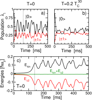
Figure 2: (color online) Spin dynamics for the initial configuration $(\lambda_{1},\lambda_{0},\lambda_{-1})=(5\%,90\%,5\%)$ and $\theta=0$. Relative populations as a function of time for (a) $T=0$ and (b) $T=0.2T_{c}^{3D}$. (c) Evolution of the kinetic (black) and $E_{c2}$ (red or dark grey) energies, and their sum (green or gray) at $T=0$. The vertical lines are at $t_{dom}$.

It is interesting to note the formation of spin domains despite the total density profile remaining almost unchanged Mur06 ; Saito05 . Hence, spin domains are linked to the kinetic and spin-spin energy terms, since all the other contributions to the energy functional depend only on the total density. The evolution of the kinetic energy and $E_{c2}$ is shown in Fig. 2(c) as a function of time for the first 500 ms. Clearly the appearence of domains is linked to a rapid variation of kinetic and $E_{c2}$ energies. Moreover, since the system has no dissipation at $T=0$, the total energy has to be conserved, and therefore, the energy difference between the starting and the equilibrium configurations provides an upper bound to the energy associated with the formation of spin domains. Actually this energy is always rather small, as can be seen in the figure. In the case of Fig. 2, the excess energy amounts to 0.28$\hbar\omega_{z}$ which represents a $0.3\%$ of the total energy.

We incorporate now finite-temperature effects by means of a Bogoliubov-de Gennes description of the thermal clouds. Further we assume that each spin component has its own cloud Tfinita , and solve the corresponding time-dependent equations under these conditions Mur06 . With our choice of parameters, the condensation in an elongated trap occurs at $k_{B}T_{c}^{3D}\approx 0.94\hbar\omega_{ho}N^{1/3}$, where $\omega_{ho}=(\omega_{\perp}^{2}\omega_{z})^{1/3}$ Vandruten96 . In Fig. 2(b) we show for $T=0.2T_{c}^{3D}$ the time evolution of the relative populations, starting from the same initial parameters as in the $T=0$ case. It is worth noticing that even if $T\gtrsim\hbar\omega_{\perp}$, the quasi-one-dimensional description of the thermal effects is still valid Dettmer01 .

A simple comparison between Fig. 2(a) and 2(b) shows that at finite $T$ the oscillations in the populations are clearly damped and that the steady state configuration that is reached is different from the one at $T=0$. In particular, in Fig. 2(b) we observe that starting from the same initial configuration $(5\%,90\%,5\%)$, the long-time population distribution changes from $(25\%,50\%,25\%)$ at $T=0$ to a steady configuration with all $m$-states almost equally populated (equipartition). Moreover, even though the local magnetization is no longer conserved as it was at $T=0$ Mur06 , the total magnetization is still a conserved quantity along all the time evolution. In general, temperature effects reflect in a faster damping and in an earlier domain formation in comparison to $T=0$. A way to understand this result is to assume that the steady configuration is attained by maximizing the entropy, subjected to the conservation of total population and magnetization:

$$\bar{S}=-\sum_{m}\lambda_{m}\ln(\lambda_{m})-\Lambda\big{(}\sum_{m}m\lambda_{m}-{\cal M}\big{)}-\mu\big{(}\sum_{m}\lambda_{m}-1\big{)},$$

where we have introduced the Lagrange multipliers $\Lambda$ and $\mu$ associated with the magnetization and the normalization, respectively. Imposing that ${\partial\bar{S}}/{\partial\lambda_{m}}=0$, together with the normalization and magnetization constraints, leads to the following condition for the steady state configurations:

$${\cal M}^{2}=1-2\lambda_{0}-3\lambda_{0}^{2},$$ (5)

which corresponds to the dot-dashed curve plotted in Fig. 1. Notice that the curve thus obtained is independent of temperature. However, the hypothesis underlying its derivation is appropriate for a high temperature regime. Therefore, one expects that this curve together with the one for the $T=0$ case [Eq. (4)] limit the zone of the configurations around which the system will oscillate depending on temperature. In fact, the results of our numerical simulations for different temperatures and initial configurations, shown in Fig. 1, are spread between the two curves. We present results for $T/T_{c}^{3D}=0.05$ (rhombi), 0.1 (squares), 0.2 (triangles) and 0.4 (inverted triangles). For a given initial configuration, when the temperature increases, the steady state gets closer to the curve of maximum entropy. This is illustrated for ${\cal M}=0.2$ and 0.4. In both cases, the initial configuration is indicated by open squares. Notice that for ${\cal M}=0.2$, the initial configuration is on the equilibrium curve ($T=0$) and its evolution is a direct consequence of the temperature. Also one observes a larger dependence of the final steady state configuration on the initial conditions than at $T=0$. In the figure, this is illustrated for ${\cal M}=0,$ and $0.1$ by the presence of more than one symbol belonging to the same temperature that correspond to different initial conditions.

Summarizing, we have shown that at zero temperature and in absence of external magnetic fields the spin populations of $F=1$ condensates oscillate around a steady state which is well determined by analyzing the simpler homogeneous case. This steady state is close to the one described by minimizing the $E_{c2}$ energy at constant magnetization for the homogeneous case [Eq. (4)]. In confined systems, spin domain formation is associated to the excess of spin-spin coupling energy, which converts into kinetic energy back and forward dynamically.

At finite $T$, the condensate exchanges energy with the thermal clouds, and the system evolves towards a different steady state configuration which depends also on the temperature. We have shown, however, that the configurations defined on the homogenous case by minimization of the energy and maximization of the entropy set an upper and lower bound on the accessible steady state configurations for confined spinor condensates at finite $T$. These predictions can serve as a guide for the interpretation of on-going experiments on spinor condensates.

We thank K. Bongs and K. Sengstock for illuminating remarks. We acknowledge financial support by Spanish MEC Grants No. FIS2005-03142/01414/01369/04627 and CONSOLIDER INGENIO2010 CDS2006-00019 “QOIT”, by Generalitat de Catalunya Grants No. 2005SGR-00343/00185, by the EU network “Cold Molecules” (HPRN-CT-2002-00290) and IST/FET/QIPC Integrated Project “SCALA”, and by the ESF Programme “QUDEDIS”. Laboratoire Aimé Cotton is part of the Fédération LUMAT and of IFRAF.

References

- (1) See M. Lewenstein et al., Adv. Phys. 56, 243 (2007).
- (2) J. Mur-Petit et al., Phys. Rev. A 73, 013629 (2006).
- (3) H. Pu et al., Phys. Rev. A 60, 1463 (1999).
- (4) M. S. Chang et al., Nature Physics 1, 111 (2005).
- (5) M. S. Chang et al., Phys. Rev. Lett. 92, 140403 (2004).
- (6) T.-L. Ho, Phys. Rev. Lett. 81, 742 (1998).
- (7) T. Ohmi and K. Machida, J. Phys. Soc. Jpn. 67, 1822 (1998); T. Isoshima, K. Machida, and T. Ohmi, Phys. Rev. A 60, 4857 (1999).
- (8) H. Schmaljohann et al., Phys. Rev. Lett. 92, 040402 (2004); T. Kuwamoto, K. Araki, T. Eno, and T. Hirano Phys. Rev. A 69, 063604 (2004).
- (9) J. M. Higbie et al., Phys. Rev. Lett. 95, 050401 (2005).
- (10) In the transverse Thomas-Fermi (TF) limit (), should be replaced by the TF radius, cf. Ref. You12005 .
- (11) W. Zhang and L. You, Phys. Rev. A 71, 025603 (2005).
- (12) S. Yi, Ö. E. Müstecaplioglu, C.P. Sun, and L. You, Phys. Rev. A 66, 011601(R) (2002).
- (13) W. Zhang et al., Phys. Rev. A 72, 013602 (2005).
- (14) N. P. Robins, W. Zhang, E. A. Ostrovskaya, and Y. S. Kivshar, Phys. Rev. A 64, 021601(R) (2001).
- (15) H. Saito and M. Ueda, Phys. Rev. A 72, 023610 (2005).
- (16) W. Zhang et al., Phys. Rev. Lett. 95, 180403 (2005).
- (17) M. Erhard et al., Phys. Rev. A 70, 031602(R) (2004).
- (18) W. Ketterle and N. J. van Druten, Phys. Rev. A 54, 656 (1996).
- (19) D. S. Petrov, D. M. Gangardt, and G. V. Shlyapnikov, J. Phys. IV 116, 5 (2004); for comparison with experimental data see S. Dettmer et al. Phys. Rev. Lett. 87, 160406 (2001).