Formation and growth of clusters in colloidal suspensions

Abstract

Depending on the $p\mathrm{H}$-value and salt concentration of Al₂O₃ suspensions different microstructures can form. Especially the clustered one is of major interest for industrial purposes as found in the production of ceramics. In this paper we investigate the clustered microstructure by means of a coupled Stochastic Rotation Dynamics (SRD) and Molecular Dynamics (MD) simulation. In order to gain statistics within a system containing numerous clusters, large simulation volumes are needed. We present our parallel implementation of the simulation algorithm as well as a newly developed cluster detection and tracking algorithm. We then show first results of measured growth rates and cluster size distributions to validate the applicability of our method.

PACS Nos.: 82.70.-y, 47.11.+j, 02.70.Ns

1 Introduction

Colloidal suspensions in general are present everywhere in our daily life. Paintings, cosmetic products, and different kinds of food are some examples. They behave in a complex way, since different time and length scales are involved. The particle sizes are on a mesoscopic length scale, i.e., in the range of nanometers up to micrometers. Depending on the particle sizes, materials, and concentrations, different interactions are of relevance and often several of them are in a subtle interplay: electrostatic repulsion, depletion forces, van der Waals attraction, hydrodynamic interaction, Brownian motion, and gravity are the most important influences. Here, we are interested in colloids, where attractive van der Waals interaction is important for the description, i.e., where under certain circumstances cluster formation plays an important role[1, 2]. To model these systems experimentally, Al₂O₃ suspensions are commonly used[3, 4]. Al₂O₃ is also a common material in the ceramics industry. There, wet processing of suspensions, followed by a sinter process is a common practice. The stability of the resulting workpiece strongly depends on the properties of the clusters formed before the sintering process. The size distribution, stability and local porosity of the clusters as well as the time dependence of their formation are only a few of the parameters of influence.

In our work we investigate cluster formation of a sheared solution of spherical Al₂O₃ particles of diameter $0.37\,\mu$m in water. Cluster formation can have different reasons: depletion forces[5, 6, 7], like-charge attraction mediated by the counterions in the solvent[8, 9, 10], or, as in our case, van der Waals attraction[11, 12, 13]. The shear flow can either support cluster formation at low shear rates, or it can suppress cluster formation at high shear rates as we have shown in [14]. We adjust the simulation parameters so that the simulation corresponds quantitatively to a real suspension with 5% volume concentration under shear. The shear rate is kept fixed at $\dot{\gamma}=20\mathrm{/s}$[15, 16]. For Al₂O₃ suspensions attractive van der Waals forces compete with electrostatic repulsion. Depending on the particle surface charge, clustering due to attractive van der Waals forces can dominate or be prevented. We have presented how one can relate parameters of DLVO potentials[17, 18] with experimentally tunable parameters, i.e., the $p\mathrm{H}$-value and the salt concentration expressed by the ionic strength $I$, influence the charge of the colloidal particles[16]. We explored the stability diagram of Al₂O₃ suspensions and reproduced that the particles are uncharged close to the so called “isoelectric point” at $p\mathrm{H}=8.7$, where they form clusters regardless of the ionic strength. For lower $p\mathrm{H}$-values particles can be stabilized in solution. For very low $p\mathrm{H}$-values, low salt concentrations, and high volume fractions a repulsive structure can be found. The particle size is on a mesoscopic length scale, where Brownian motion is relevant and long range hydrodynamic interactions are of importance. Therefore, we use “Stochastic Rotation Dynamics” (SRD), which includes both, hydrodynamics and Brownian motion for the description of the fluid solvent[19, 20].

2 Simulation algorithm

Our simulation method is described in detail in[15, 16] and consists of two parts: a Molecular Dynamics (MD) code, which treats the colloidal particles, and a Stochastic Rotation Dynamics (SRD) simulation for the fluid solvent. In the MD part we include effective electrostatic interactions and van der Waals attraction, known as DLVO potentials[17, 18], a lubrication force and Hertzian contact forces. DLVO potentials are composed of two terms, the first one being an exponentially screened Coulomb potential due to the surface charge of the suspended particles

$$V_{\mathrm{Coul}}=\pi\varepsilon_{r}\varepsilon_{0}\left[\frac{2+\kappa d}{1+\kappa d}\cdot\frac{4k_{\mathrm{B}}T}{ze}\tanh\left(\frac{ze\zeta}{4k_{\mathrm{B}}T}\right)\right]^{2}\times\frac{d^{2}}{r}\exp(-\kappa[r-d]),$$ (1)

where $d$ denotes the particle diameter, $r$ the distance between the particle centers, $e$ the elementary charge, $T$ the temperature, $k_{\mathrm{B}}$ the Boltzmann constant, and $z$ is the valency of the ions of added salt. $\varepsilon_{0}$ is the permittivity of the vacuum, $\varepsilon_{r}=81$ the relative dielectric constant of the solvent, $\kappa$ the inverse Debye length defined by $\kappa^{2}=8\pi\ell_{B}I$, with ionic strength $I$ and Bjerrum length $\ell_{B}=7\,\mathrm{\AA}$. The first fraction in Eq. (1) is a correction to the DLVO potential (in the form used in[11]), which takes the surface curvature into account and is valid for spherical particles. The effective surface potential $\zeta$ can be related to the $p\mathrm{H}$-value of the solvent with a $2pK$ charge regulation model[16]. The Coulomb term competes with the attractive van der Waals interaction ($A_{\mathrm{H}}=4.76\cdot 10^{-20}\,\mathrm{J}$ is the Hamaker constant)[11]

$$V_{\mathrm{VdW}}=-\frac{A_{\mathrm{H}}}{12}\left[\frac{d^{2}}{r^{2}-d^{2}}+\frac{d^{2}}{r^{2}}\right.\;\left.+2\ln\left(\frac{r^{2}-d^{2}}{r^{2}}\right)\right].$$ (2)

The attractive contribution $V_{\mathrm{VdW}}$ is responsible for the cluster formation we observe. However, depending on the $p\mathrm{H}$-value and the ionic strength, it may be overcompensated by the electrostatic repulsion. When particles get in contact, the potential has a minimum. However, Eq. (2) diverges due to the limitations of DLVO theory. We cut off the DLVO potentials and model the minimum by a parabola. The particle contacts are modeled as Hertzian contacts and for non-touching particles, below the resolution of the SRD algorithm short range hydrodynamics is corrected by a lubrication force, which we apply within the MD framework, as we have explained in Ref.  [15, 16]. For the integration of translational motion of the colloidal particles we utilize a velocity Verlet algorithm[21] and for the fluid we apply the Stochastic Rotation Dynamics method (SRD)[19, 20]. It intrinsically contains fluctuations, is easy to implement, and has been shown to be well suitable for simulations of colloidal and polymer suspensions[22, 23, 24, 25, 15, 16]. The method is also known as “Real-coded Lattice Gas”[22] or as “multi-particle-collision dynamics” (MPCD)[24] and is based on coarse-grained fluid particles with continuous positions and velocities. A streaming step and an interaction step are performed alternately. In the streaming step, each particle $i$ is moved according to $\mathbf{r}_{i}(t+\tau)=\mathbf{r}_{i}(t)+\tau\;\mathbf{v}_{i}(t)$, where $\mathbf{r}_{i}(t)$ denotes the position of the particle $i$ at time $t$ and $\tau$ is the time step. In the interaction step fluid particles are sorted into cubic cells of a regular lattice and only the particles within the same cell interact according to an artifical collision rule which conserved energy and momentum. First, for each independent cell $j$ the mean velocity $\mathbf{u}_{j}(t^{\prime})=\frac{1}{N_{j}(t^{\prime})}\sum^{N_{j}(t^{\prime})}_{i=1}\mathbf{v}_{i}(t)$ is calculated. $N_{j}(t^{\prime})$ is the number of fluid particles contained in cell $j$ at time $t^{\prime}=t+\tau$. Then, the velocities of each fluid particle are rotated according to

$$\mathbf{v}_{i}(t+\tau)=\mathbf{u}_{j}(t^{\prime})+\mathbf{\Omega}_{j}(t^{\prime})\cdot[\mathbf{v}_{i}(t)-\mathbf{u}_{j}(t^{\prime})].$$ (3)

$\mathbf{\Omega}_{j}(t^{\prime})$ is a rotation matrix, which is independently chosen at random for each time step and cell. Rotations are about one coordinate axes by a fixed angle $\pm\alpha$. To couple colloidal particles and the fluid, the particles are sorted into SRD cells and their velocities are included in the rotation step. The masses of colloidal and fluid particles are used as a weight factor for the mean velocity

$$\mathbf{u}_{j}(t^{\prime})=\frac{1}{M_{j}(t^{\prime})}\sum\limits^{N_{j}(t^{\prime})}_{i=1}\mathbf{v}_{i}(t)m_{i},\qquad\mathrm{with}\qquad M_{j}(t^{\prime})=\sum^{N_{j}(t^{\prime})}_{i=1}m_{i}.$$ (4)

We sum over all colloidal and fluid particles in the cell to obtain their total number $N_{j}(t^{\prime})$. $m_{i}$ is the mass of particle $i$ and $M_{j}(t^{\prime})$ gives the total mass contained in cell $j$ at time $t^{\prime}=t+\tau$. We apply shear by explicitly setting the mean velocity $\mathbf{u}_{j}$ to the shear velocity in the cells close to the border of the system. A thermostat removes the energy introduced to the system by the shear force.

A single simulation run as presented in our previous papers took between one and seven days on a 3GHz Pentium CPU. However, for strongly clustering systems we easily end up with only a single cluster inside the simulation volume. In order to be able to gather statistics on cluster growth and formation, as well as to minimize finite size effects, we parallelized our code. While MD codes have been parallelized by many groups, only few parallel implementations of a coupled MD and SRD program exist. This is in contrast to the number of parallel implementations of other mesoscopic simulation methods like for example the lattice Boltzmann method. A possible explanation is that SRD is a more recent and so far not as widely used algorithm causing the parallelization to be a more challenging task. In order to push the development in this field we provide some details of our implementation in this section.

We utilize the Message Pasing Interface (MPI) to create a C++ code based on domain decomposition for both involved simulation methods. In the MD code the position of neighbouring particles is needed to compute the interactions. Since the intractions have a limited range, and a linked cell algorithm is already used in the serial code, we apply linked cells here as well. Particle positions at the border of the domain of each processor are communicated to the neighbouring processors for the calculation of the forces. Then, the propagation step is performed and particle positions are updated, whereby the particles crossing a domain boundary are transferred from one processor to the other one.

Since (in principle), fluid particles can travel arbitrary large distances in one time step, one either has to limit the distance they can move, or one needs all-to-all communication between the processors. Even though the mean free path in our systems is small enough to limit communication to nearest neighbours only, the current version of our code tries to be as general as possible and allows fluid particles to move to any possible position in the total simulation volume within a single timestep. First, we determine locally which fluid particles have to be sent to which destination CPU and collect all particles to be sent to the same destination into a single MPI message. If no particles are to be sent, a zero dummy message is transmitted. On the receiving side, MPI_Probe with the MPI_ANY_SOURCE option is utilized to determine the sender’s rank and the number of particles to be accomodated. Now, MPI_Recv can be used to actually receive the message. All processors send and receive in arbitrary order, thus waiting times are kept at a minimum allowing a very efficient communication. The standard MPI all-to-all communication procedure should be less efficient since the size of every message would be given by the size of the largest message. However, we still do find a substantial communication overhead from our benchmark tests of the scalability of the code. Due to this overhead, we are currently limited to 32-64 CPUs on an IBM p690 cluster. In order to achieve Gallilean invariance, a random shift of the SRD lattice is performed for every rotation step[26, 27]. Since the domains managed by each CPU do not move, this would include the borders between the processors to cross SRD cells, which is undesirable. Therefore, we keep the position of the lattice fixed and shift the fluid particle positions before sorting them into the cells instead. After the rotation step they are shifted back.

3 Results

We study the formation of clusters for systems containing a volume concentration of $5\%$ of colloidal particles (=1320 MD particles), a shear rate of $\dot{\gamma}=20\mathrm{/s}$, ionic strengths $I=3\mathrm{mmol/l}$ and $7\mathrm{mmol/l}$, and $p\mathrm{H}=6$ and $7$. To demonstrate the effect of clustering, in Fig. 1 snapshots from a typical simulation of a $8.88\mu\mathrm{m}^{3}$ system with periodic boundaries at $I=7\mathrm{mmol/l}$ and $p\mathrm{H}=6$ at different times are shown. While at the beginning of the simulation (a), freely moving particles can be observed, small clusters appear after $t=0.26$s (b). After $t=1.06$s, all particles are contained within three individual clusters (c) and after $t=4.22$s only a single cluster is left in the system. For an investigation of the formation and movement of clusters, substantially larger systems are needed. Therefore, we scale up the simulation volume to $17.76\mu\mathrm{m}^{3}$ containing 10560 MD particles and 1.3$\cdot$10⁷ fluid particles. Due to the computational demands of the fluid solver, a single simulation of $5$s real time requires about 5000 CPU hours on 32 CPUs of an IBM p690 system.

a)  $t=0.05$s                              b)  $t=0.26$s

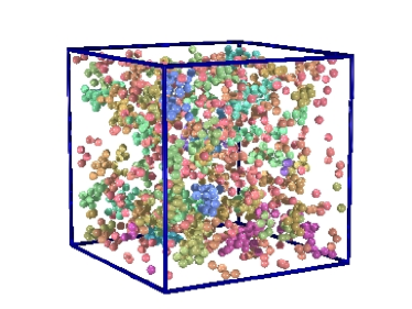
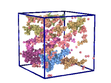
c)  $t=1.06$s                              d)  $t=4.22$s

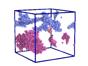
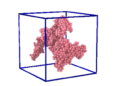
Figure 1: Snapshots of a simulation of an $8.88\mu\mathrm{m}^{3}$ system, filled with $\Phi=5\%$ MD particles of diameter $d=0.37\mu\mathrm{m}$ under shear with $\dot{\gamma}=20\mathrm{/s}$.

We developed a cluster detection algorithm which not only examines a certain configuration at a fixed time, but also takes account of the time evolution of clusters. This algorithm works as follows: a cutoff radius is introduced, below which two particles are considered to be connected. If they are separated further, they are considered as being not directly connected. However, they might both be connected to a third particle. Therefore we have to check all particle pairs for possible connections. If there are no further connections, the particles are considered not to belong to any cluster. Otherwise four cases have to be distinguished: If both particles are not part of any cluster, a new cluster is created and both particles are assigned to it (1). If one particle is already part of a cluster, the other one is assigned to the same cluster (2). If both particles belong to different clusters, the clusters are united, i.e., all particles of the smaller cluster are assigned to the larger one (3). If it is found that for a particle pair to be checked later on, both particles already belong to the same cluster, nothing has to be done (4). This pairwise checking is optimized by a linked cell algorithm, so that only particle pairs of the same and of neighbouring cells are checked. Additionally, clusters need to be tracked in time, i.e., the clusters found within a time step have to be identified with the clusters of the previous time step. This is done by assigning an identification number (“cluster ID”) for every cluster. Since every particle has a unique identification number, assigning the ID of the cluster it belongs to solves the problem. According to which cluster ID the particles were assigned in the previous time step, the ID is assigned to the new cluster. Again four different cases have to be considered: if both particles belonged to the same cluster, and therefore refer to the same cluster ID, this ID is assigned to the new cluster (1). If one of the particles did not belong to any cluster in the previous time step, a new cluster has formed during the last time step and has to be provided with a new ID (2). If only one particle was part of a cluster, the ID it provides is preserved (3). If the particles are assigned to different cluster IDs one of those IDs has to be choosen for the new cluster. We decide for the one referring to the larger cluster of the previous time step or choose randomly if both clusters are of identical size (4). Finally one has to check if the cluster IDs are unique. If several clusters are assigned to the same id the largest one keeps the ID and the smaller ones are assigned to new ones.

The strength of our algorithm is the possibility to track individual particles and their assignment to different clusters in time. Clusters grow and break into pieces and we can follow the trajectory of each particle in this scenario. This enables us to draw cluster assignment trees like the one in Fig. 2. In contrast to conventional algorithms, where clusters cannot be tracked in time, the clusters are sorted here on the $x$ axis and keep their position. The lines are obtained by plotting the assignment of the particles to the clusters and their distance depicts the cluster sizes, i.e., if at time $t$ a cluster contains a fraction $p$ of all particles in the simulation, a fraction $p$ is reserved for this cluster on the $x$-axis and the line is plotted at the center of this region. Consequently, if only a single cluster is left in the system, the corresponding line is drawn at $x=0.5$. Depending on the inter particle forces, different structures can be identified, meaning different scenarios like breaking up of large clusters or unification of smaller ones. We are planning to study systematically the dependence of the structures seen in such cluster tree plots on the inter particle forces determined by the $p\mathrm{H}$-value and the ionic strength $I$ in a future work.

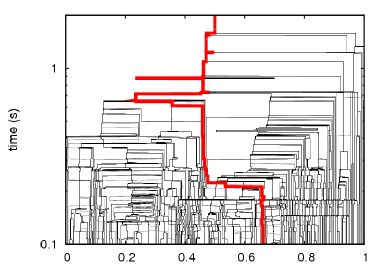
Figure 2: Tree-like structure of the assignment of colloidal particles to individual clusters. This cluster tree corresponds to the simulation presented in Fig. 1. For better visibility, the time is given on a logarithmic scale. All particles start at the bottom of the plot and aggregate in individual clusters as shown by the merging lines. After two seconds, only a single large cluster is left in the system. The thick line denotes the path of a single particle in order to demonstrate the possibility to track which cluster this particle belongs to and how these clusters break up and remerge.

In Fig. 3 we present the time dependence of the mean cluster size (a) and of the number of clusters in the system (b). We find that both observables can be fitted by a power law of the form $A\cdot(t+B)^{C}$, where $A,B,C$ are fitting parameters. The lines in the figure correspond to the fit and the symbols to the simulation data. The parameters $A,B,C$ to fit the simulation data shown in Fig. 3 are listed in table 3. It would be of great interest to investigate if a general scaling behavior can be observed depending on the volume concentration, the ionic strength and the pH value. However, for this a detailed investigation of the parameter space would be needed which will be the focus of a future work.

a)                                                     b)

Figure 3: The time dependence of the mean cluster size is plotted for different simulation parameters (a). Fig. b) depicts the time dependence of the number of clusters found in the system. Each curve is shifted vertically by a factor of two for better visibility. While the symbols correspond to simulation data, lines are given by a power law fit.

conditions		number of clusters			mean cluster size
$p\mathrm{H}$	$\frac{I}{\mathrm{mmol/l}}$	$A$	$B/\mathrm{ms}$	$C$	$A$	$B/\mathrm{ms}$	$C$
6	3	$1.5\cdot 10^{6}$	71	-1.25	$3.27\cdot 10^{-3}$	96	1.36
7	3	$5.27\cdot 10^{7}$	131	-1.9	$8.42\cdot 10^{-7}$	277	2.66
6	7	$1.46\cdot 10^{8}$	142	-2.047	$8.05\cdot 10^{-7}$	277	2.66
7	7	$1.01\cdot 10^{8}$	162	-1.98	$8.72\cdot 10^{-7}$	277	2.66

Table 1. Parameters for the fit of the simulation data

4 Conclusion

In this paper we have demonstrated an efficient way to parallelize a combined SRD and MD code and presented our new cluster detection algorithm that is able to not only detect clusters, but also to track their positions in time. We applied this algorithm to data obtained from large scale simulations of colloidal suspensions in the clustering regime and find that the time dependence of the mean cluster size and the number of clusters in the system can be well described by power laws.

References

- [1] W. B. Russel, D. A. Saville, and W. Schowalter. Colloidal Dispersions. Cambridge University Press, 1995.
- [2] R. J. Hunter. Foundations of colloid science. Oxford University Press, Oxford, 2001.
- [3] S. Richter and G. Huber. Resonant column experiments with fine-grained model material - evidence of particle surface forces. Granular Matter, 5:121–128, 2003.
- [4] S. Richter. Mechanical Behavior of Fine-grained Model Material During Cyclic Shearing. PhD thesis, University of Karlsruhe, Germany, 2006.
- [5] X. Ye, T. Narayanan, P. Tong, J. S. Huang, M. Y. Lin, B. L. Carvalho, and L. J. Fetters. Depletion interactions in colloid-polymer mixtures. Phys. Rev. E, 54:6500, 1996.
- [6] R. Tuinier, G. A. Vliegenthart, and H. N. W. Lekkerkerker. Depletion interaction between spheres immersed in a solution of ideal polymer chains. J. Chem. Phys., 113:10768, 2000.
- [7] D. Rudhardt, C. Bechinger, and P. Leiderer. Direct measurement of depletion potentials in mixtures of colloids and nonionic polymers. Phys. Rev. Lett., 81:1330, 1998.
- [8] B. V. R. Tata, M. Rajalakshmi, and A. K. Arora. Vapor-liquid condensation in charged colloidal syspensions. Phys. Rev. Lett., 69(26):3778, 1992.
- [9] B. V. R. Tata, E. Yamahara, P. V. Rajamani, and N. Ise. Amorphous clustering in highly charged dilute poly(chlorostyrene-styrene sulfonate) colloids. Phys. Rev. Lett., 78(13):2660, 1997.
- [10] P. Linse and V. Lobaskin. Electrostatic attraction and phase separation in solutions of like-charged colloidal particles. Phys. Rev. Lett., 83(20):4208, 1999.
- [11] M. Hütter. Brownian Dynamics Simulation of Stable and of Coagulating Colloids in Aqueous Suspension. PhD thesis, Swiss Federal Institute of Technology Zurich, 1999.
- [12] G. Wang, P. Sarkar, and P. S. Nicholson. Surface chemistry and rheology of electrostatically (ionically) stabillized alumina suspensions in polar media. J. Am. Ceram. Soc., 82(4):849–56, 1999.
- [13] M. Hütter. Local structure evolution in particle network formation studied by brownian dynamics simulation. J. Colloid Interface Sci., 231:337–350, 2000.
- [14] M. Hecht, J. Harting, and H. J. Herrmann. A stability diagram for dense colloidal al2o3-suspensions in shear flow. arXiv:cond-mat/0606455, 2006.
- [15] M. Hecht, J. Harting, T. Ihle, and H. J. Herrmann. Simulation of claylike colloids. Phys. Rev. E, 72:011408, jul 2005.
- [16] M. Hecht, J. Harting, M. Bier, J. Reinshagen, and H. J. Herrmann. Shear viscosity of clay-like colloids in computer simulations and experiments. Phys. Rev. E, 74:021403, 2006.
- [17] E. J. W. Vervey and J. T. G. Overbeek. Theory of the Stability of Lyophobic Colloids. Elsevier, Amsterdam, 1948.
- [18] B. V. Derjaguin and L. D. Landau. Theory of the stability of strongly charged lyophobic sols and of the adhesion of strongly charged particles in solutions of electrolytes. Acta Phsicochimica USSR, 14:633, 1941.
- [19] A. Malevanets and R. Kapral. Mesoscopic model for solvent dynamics. J. Chem. Phys., 110:8605, 1999.
- [20] A. Malevanets and R. Kapral. Solute molecular dynamics in a mesoscale solvent. J. Chem. Phys., 112:7260, 2000.
- [21] M. P. Allen and D. J. Tildesley. Computer simulation of liquids. Oxford Science Publications. Clarendon Press, Oxford, 1987.
- [22] Y. Inoue, Y. Chen, and H. Ohashi. Development of a simulation model for solid objects suspended in a fluctuating fluid. J. Stat. Phys., 107(1):85–100, 2002.
- [23] J. T. Padding and A. A. Louis. Hydrodynamic and brownian fluctuations in sedimenting suspensions. Phys. Rev. Lett., 93:220601, 2004.
- [24] M. Ripoll, K. Mussawisade, R. G. Winkler, and G. Gompper. Dynamic regimes of fluids simulated by multiparticle-collision dynamics. Phys. Rev. E, 72:016701, 2005.
- [25] I. Ali, D. Marenduzzo, and J. M. Yeomans. Dynamics of polymer packaging. J. Chem. Phys., 121:8635–8641, November 2004.
- [26] T. Ihle and D. M. Kroll. Stochastic rotation dynamics I: Formalism, galilean invariance, green-kubo relations. Phys. Rev. E, 67(6):066705, 2003.
- [27] T. Ihle and D. M. Kroll. Stochastic rotation dynamics II: Transport coefficients, numerics, long time tails. Phys. Rev. E, 67(6):066706, 2003.