Coherence oscillations in dephasing by non-Gaussian shot noise

Abstract

A non-perturbative treatment is developed for the dephasing produced by the shot noise of a one-dimensional electron channel. It is applied to two systems: a charge qubit and the electronic Mach-Zehnder interferometer, both of them interacting with an adjacent partitioned electronic channel acting as a detector. We find that the visibility (interference contrast) can display oscillations as a function of detector voltage and interaction time. This is a unique consequence of the non-Gaussian properties of the shot noise, and only occurs in the strong coupling regime, when the phase contributed by a single electron exceeds $\pi$. The resulting formula reproduces the recent surprising experimental observations reported in [I. Neder et al., cond-mat/0610634], and indicates a general explanation for similar visibility oscillations observed earlier in the Mach-Zehnder interferometer at large bias voltage. We explore in detail the full pattern of oscillations as a function of coupling strength, voltage and time, which might be observable in future experiments.

(1) Braun Center for Submicron Research, Department of Condensed Matter Physics, Weizmann Institute of Science, Rehovot 76100, Israel
(2) Physics Department, Center for NanoScience, and Arnold Sommerfeld Center for Theoretical Physics, Ludwig-Maximilians Universität München, Theresienstr. 37, 80333 Munich, Germany

1 Introduction

Decoherence, i.e. the destruction of quantum mechanical interference effects, is a topic whose importance ranges from more fundamental questions like the quantum-classical crossover to possible applications of quantum coherent phenomena, such as sensitive measurements and quantum information and quantum computing. In mesoscopic transport experiments, decoherence (also called dephasing) is responsible for the nontrivial temperature- and voltage-dependence of the electrical conductance in disordered samples (displaying weak localization and universal conductance fluctuations) and solid-state electron interferometers.

The most important paradigmatic quantum-dissipative models (“Caldeira-Leggett” [1, 2] and “spin-boson” [3, 4]) and many well-known techniques used for describing decoherence assume the environment to be a bath of harmonic oscillators, where the fluctuations obey Gaussian statistics. This assumption is correct for some cases (e.g. photons and phonons), and generally represents a very good approximation for the combined contribution of many weakly coupled fluctuators, due to the central limit theorem. However, ultrasmall structures may couple only to a few fluctuators (spins, charged defects etc.), thus requiring models of dephasing by non-Gaussian noise. Such models are becoming very important right now in the context of quantum information processing [5, 6, 7, 8, 9, 10, 11, 12, 13, 14].

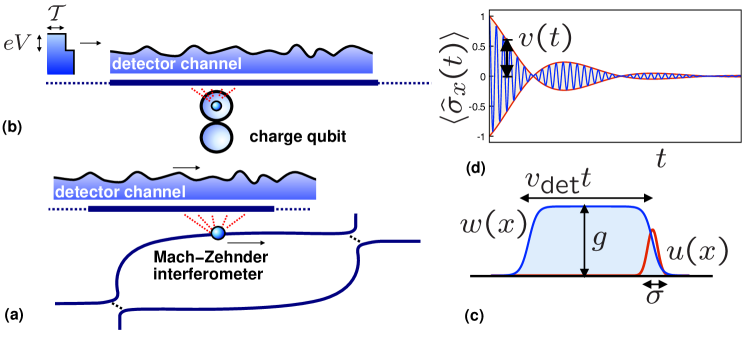
Figure 1: Schematic drawing of the models considered in the text: A detector channel with shot noise coupled to (a) an interferometer channel or (b) a charge qubit. (c) The interaction potential $u(x)$ defines the phase function $w(x)$, whose height gives the dimensionless coupling constant $g$, see equation (18). (d) Sketch of the time-evolution of the oscillations in $\left\langle\hat{\sigma}_{x}(t)\right\rangle$, indicating the visibility $v(t)$ as the magnitude of the oscillation envelope. In this schematic example, the visibility itself oscillates - this is impossible in models of Gaussian noise but a direct feature of the non-Gaussian nature of the shot noise, in the strong coupling regime $g>\pi$ (see text and following figures).

Moreover, the quantum measurement process itself is accompanied by unavoidable fluctuations which dephase the quantum system [15, 16, 17], while dephasing itself can conversely be viewed as a kind of detection process [18, 19]. Therefore, ”controlled dephasing” experiments can be used to study the transition from quantum to classical behavior, e.g. by coupling an electron interferometer to a tunable “which path detector” [20, 21, 22, 23, 24, 25], which produces shot noise by partitioning an electron stream [26, 27, 28, 29, 30]. In previous mesoscopic controlled dephasing experiments the coupling between detector and interferometer was weak, requiring the passage of many detector electrons in order to determine the path. Under these conditions, the phase of the interfering electron fluctuates according to a Gaussian random process.

Recently, a controlled dephasing experiment was performed [31, 32] using an electronic Mach-Zehnder Interferometer (MZI) [33, 34] coupled to a nearby partitioned edge-channel serving as a detector. Its results differed substantially from those of earlier controlled-dephasing experiments. The interference contrast of the Aharonov-Bohm oscillations, quantified by the visibility $v=(I_{{\rm max}}-I_{{\rm min}})/(I_{{\rm max}}+I_{{\rm min}})$, revealed two unexpected effects:

(a) The visibility as a function of the detector transmission probability $\mathcal{T}$ changes from the expected smooth parabolic suppression $\propto\mathcal{T}(1-\mathcal{T})$ at low detector voltages to a sharp “V-shape” behaviour at some larger voltages.

(b) The visibility drops to zero at intermediate voltages, then reappears again as $V$ increases, and vanishes at even larger voltages, thus displaying oscillations.

As estimated in [31], three (or even fewer) detecting electrons suffice to quench the visibility. For this reason, one suspects that these effects may be a signature of the strong coupling between interferometer and detector. Indeed, that coupling has already been exploited to entangle the interfering electrons with the detector electrons, and afterwards recover the phase information by cross-correlating the current fluctuations of the MZI and the detector [31], even after it has completely vanished in conductance measurements. The dephasing in the MZI system is caused by the detector’s shot noise, which is known to obey binomial, i.e. non-Gaussian, statistics. Thus, earlier theoretical discussions of dephasing in the electronic Mach-Zehnder interferometer, based on a Gaussian environment [35, 36, 37, 38, 39, 40], are no longer sufficient (see [41, 42] for a discussion of Luttinger liquid physics in an MZI). At the same time, a nonperturbative treatment is required, to capture the non-Gaussian effects. Higher moments of the noise become important, and dephasing starts to depend on the full counting statistics, which itself represents a topic attracting considerable attention nowadays [43, 39, 44]. The relation between full counting statistics, detection and dephasing has been explored recently by Averin and Sukhorukov [44]. There, the dephasing rate and the measurement rate were considered, i.e. the focus was placed on the long-time limit, similarly to other calculations of dephasing by non-Gaussian noise [5, 7, 10, 12, 13, 14]. In contrast, we will emphasize the surprising evolution of the visibility at short to intermediate times.

The main purpose of this paper then is to present a nonperturbative treatment of a theoretical model that explains the new experimental results, and provides quantitative predictions for the behavior of the visibility as a function of detector bias and partitioning. Furthermore, we will show how the approximate solution for the MZI is directly related to an exact solution for the pure dephasing of a charge qubit by shot noise, where the time evolution of the visibility parallels the evolution with detector voltage. In conclusion, it will emerge that the novel features observed in [32], and the results derived here, are in fact fundamental and generic consequences of dephasing by the non-Gaussian shot noise of a strongly coupled electron system. As a side effect, this may indicate a solution to the puzzling observation of visibility oscillations in a MZI without adjacent detector channel [34].

The paper is organized as follows: We first describe dephasing of a charge qubit, being the simpler model that can be solved exactly. After introducing the model in section 2.1, we derive the exact solution (2.2). We briefly discuss the relation to full counting statistics (2.3), and provide formulas obtained in the well-known Gaussian approximation (2.4, 2.5) for comparison, before presenting and discussing the results obtained from a numerical evaluation of the exact expression (section 2.6). In section 3, we then go on to introduce a certain approximation that keeps only the nonequilibrium part of the noise and allows an analytical discussion of many features, some of which become particularly transparent in the wave packet picture of shot noise (3.2). In section 4 we briefly contrast the features of our solution with those of the well-known model describing dephasing by classical random telegraph noise. The Mach-Zehnder interferometer is then described in section 5, by first solving exactly the problem of a single electron interacting with the detector (5.1), and then introducing the Pauli principle (5.2). The results are discussed (5.3) and compared against the experimental data (5.4). Finally, we briefly indicate (5.5) a possible solution to the puzzling visibility oscillations observed in the MZI without detector channel.

Our main results are: the exact formula for the time-evolution of the visibility of the charge qubit given in equation (19), and the formula for the effect of the nonequilibrium part of the noise on the visibility of qubit (37) or interferometer (65). Their most important general analytical consequences are derived in section 3.1, including a detailed discussion of the visibility oscillations.

2 Charge qubit subject to non-Gaussian shot noise

Interferometers may be used as highly sensitive detectors, by coupling them to a quantum system and reading out the induced phase shift. Here we focus on a setup like the one that has been realized in [23], where a double dot (“charge qubit”) has been subject to the shot noise of a partitioned one-dimensional electron channel. However, we note that the strong-coupling regime to be discussed below yet remains to be achieved in such an experiment.

2.1 Model

We consider a charge qubit with two charge states $\hat{\sigma}_{z}=\pm 1$. It is coupled to the density fluctuations of non-interacting “detector” fermions

$$\hat{H}=\hat{H}_{{\rm qb}}+\hat{H}_{{\rm int}}+\hat{H}_{{\rm det}},$$ (1)

with $\hat{H}_{{\rm qb}}=\frac{\epsilon}{2}\hat{\sigma}_{z}$,

$$\hat{H}_{{\rm det}}=\sum_{k}\epsilon_{k}\hat{d}_{k}^{\dagger}\hat{d}_{k},$$ (2)

and

$$\hat{H}_{{\rm int}}=\frac{\hat{\sigma}_{z}+1}{2}\hat{V}.$$ (3)

This coupling is of the diagonal form, i.e. it commutes with the qubit Hamiltonian, thereby leading only to pure dephasing and not to energy relaxation (the populations of the qubit levels are preserved). The derivation of the exact expressions to be analyzed below depends crucially on this type of coupling. The fluctuating quantum noise potential $\hat{V}$ introduced in (3) is related to the density of detector particles in the vicinity of the qubit, see figure 1:

$$\hat{V}=\int dx\,u(x)\hat{\rho}_{{\rm det}}(x)=\sum_{k^{\prime},k}u_{k^{\prime}k}\hat{d}_{k^{\prime}}^{\dagger}\hat{d}_{k}$$ (4)

Here $u(x)$ is the arbitrary interaction potential (whose details in a realistic situation will be determined by the screening properties of the environment), $\hat{\rho}_{{\rm det}}(x)=\hat{\psi}^{\dagger}(x)\hat{\psi}(x)$ is the detector density, and $\hat{\psi}(x)=\sum_{k}\phi_{k}(x)\hat{d}_{k}$ is the expansion in terms of the single-particle eigenstates of the detector. At this point we do not yet specify the nature of the detector, as some of the following formulas are valid in general for any non-interacting fermion system. However, ultimately the evaluations will be performed for a one-dimensional channel of fermions moving chirally at constant speed, representing our model of a “detector edge channel”. This was implemented in the integer Quantum Hall Effect two-dimensional electron gas [23, 31, 32] and can presumably be realized in other one-dimensional electron systems as well (e.g. electrons moving inside a carbon nanotube).

We are interested in describing the outcome of the following standard type of experiment in quantum coherent dynamics: Suppose we prepare the qubit in a superposition state of $\left|\uparrow\right\rangle$ and $\left|\downarrow\right\rangle$ at time $t=0$, and then switch on the interaction with the detector electrons. In effect this can be realized by applying a Rabi $\pi/2$ pulse to the qubit that is initially in the state $\left|\downarrow\right\rangle$. During the following time-evolution, the off-diagonal element $\rho_{\uparrow\downarrow}(t)$ will be affected by the coupling to the bath, experiencing decoherence. Its original oscillatory time-evolution is multiplied by a factor, that can be written as the overlap $D(t)=\left\langle\chi_{\downarrow}(t)|\chi_{\uparrow}(t)\right\rangle$ of the two detector states $\chi_{\downarrow}(t)$ and $\chi_{\uparrow}(t)$ that evolve under the action of $\hat{H}_{{\rm det}}$ and $\hat{H}_{{\rm det}}+\hat{V}$, respectively. In this way, the relation between decoherence and measurement becomes evident [18]:

$$D(t)=\left\langle e^{+i\hat{H}_{{\rm det}}t}e^{-i(\hat{H}_{{\rm det}}+\hat{V})t}\right\rangle.$$ (5)

Note that we have set $\hbar\equiv 1$. This can also be written as

$$D(t)=\left\langle\hat{T}\exp(-i\int_{0}^{t}dt^{\prime}\,\hat{V}(t^{\prime}))\right\rangle,$$ (6)

where $\hat{V}(t^{\prime})$ is the fluctuating quantum noise operator in the Heisenberg picture with respect to $\hat{H}_{{\rm det}}$, and $\hat{T}$ is the time-ordering symbol. The magnitude of this time-dependent “coherence factor” defines what we will call the “visibility”

$$v=|D(t)|.$$ (7)

The visibility (with $0\leq v\leq 1$) determines the suppression of the oscillations in any observable that is sensitive to the coherence between the two levels, e.g. $\left\langle\hat{\sigma}_{x}(t)\right\rangle={\rm Re}\rho_{\uparrow\downarrow}(t)$. This is depicted in figure 1 (d).

2.2 Time-evolution of the visibility: General expressions

The average in the coherence factor $D(t)$ displayed in equation (5) is taken with respect to the unperturbed state of the detector electrons, which may refer to a nonequilibrium situation. We will assume that this initial state can be described by independently fluctuating occupations $\hat{d}_{k}^{\dagger}\hat{d}_{k}$ of the single-particle states $k$. This assumption covers all the cases of interest to us, namely the equilibrium noise at arbitrary temperature, as well as shot noise produced by transmission of particles through a partially reflecting barrier, leading to a nonequilibrium Fermi distribution.

The average (5) can be evaluated in a variety of ways, e.g. using the linked cluster expansion applied to a time-ordered exponential. However, here we make use of a convenient formula derived by Klich [45] in the context of full counting statistics. Denoting as $\Gamma(A)\equiv\sum_{k^{\prime},k}A_{k^{\prime}k}\hat{d}_{k^{\prime}}^{\dagger}\hat{d}_{k}$ the second-quantized single-particle operator built from the transition matrix elements $A_{k^{\prime}k}$, we have [45] (for fermions)

$${\rm tr}[e^{\Gamma(A)}e^{\Gamma(B)}]={\rm det}[1+e^{\hat{A}}e^{\hat{B}}],$$ (8)

where $\hat{A}$ is the operator acting in the single-particle Hilbert space. In general, this formula allows us to obtain the average of the exponential of any single-electron operator with respect to a many-particle density matrix that does not contain correlations. Indeed, for a state with independently fluctuating occupations, we can write the many-body density matrix in an exponential form that is suitable for application of equation (8):

$$\hat{\rho} = \Pi_{k}[n_{k}\hat{d}_{k}^{\dagger}\hat{d}_{k}+(1-n_{k})(1-\hat{d}_{k}^{\dagger}\hat{d}_{k})]$$ (9)

$$= \Pi_{k}(1-n_{k})e^{\sum_{k}\hat{d}_{k}^{\dagger}\hat{d}_{k}{\rm ln}\frac{n_{k}}{1-n_{k}}},$$ (10)

where $0\leq n_{k}\leq 1$ is the probability of state $k$ being occupied (formally it is necessary to consider the limits $n_{k}\rightarrow 0$ and $n_{k}\rightarrow 1$ if needed). Inserting this expression into (8), and defining the occupation number matrix $n_{k^{\prime}k}=\delta_{k^{\prime}k}n_{k}$, we are now able to evaluate averages of the form

$${\rm tr}[e^{i\sum_{k^{\prime},k}A_{k^{\prime}k}\hat{d}_{k^{\prime}}^{\dagger}\hat{d}_{k}}\hat{\rho}] = \left(\Pi_{k}(1-n_{k})\right){\rm det}[1+e^{i\hat{A}}\frac{\hat{n}}{1-\hat{n}}]$$ (11)

$$= {\rm det}[1+(e^{i\hat{A}}-1)\hat{n}].$$ (12)

The average (5) then can be performed by identifying the product of time-evolution operators as a single unitary operator, of the form given here. Thus, we find

$$D(t)={\rm det}[1+(\hat{S}(t)-1)\hat{n}],$$ (13)

where the finite-time scattering matrix (interaction picture evolution operator) is

$$\hat{S}(t)=e^{i\hat{h}_{{\rm det}}t}e^{-i(\hat{h}_{{\rm det}}+\hat{u})t}.$$ (14)

Here $\hat{u}$ is the interaction from (4), and $\hat{h}_{{\rm det}}$ is the single-particle Hamiltonian of the detector electrons that is diagonal in the $k$-basis: $\left[h_{{\rm det}}\right]_{k^{\prime}k}=\epsilon_{k}\delta_{k^{\prime}k}$ . In principle, equation (13) allows us to evaluate the time-evolution of the coherence factor for coupling to an arbitrary noninteracting fermion system.

In practice, this involves calculating the time-dependent scattering of arbitrary incoming $k$-states from the coupling potential $u(x)$, i.e. determining the action of the scattering matrix. Note that in the case of fully occupied states ($n_{k}\equiv 1$ for all $k$), the operator $\hat{n}$ becomes the identity and the determinant reduces to the product of scattering phase factors that can be obtained by diagonalizing the scattering matrix. More generally, the contributions to $D(t)$ from states deep inside the Fermi sea always only amount to a phase factor, which will drop out when considering the visibility $v=|D(t)|$.

In the remainder of this paper, we will focus on the specific, and experimentally relevant, case of a one-dimensional channel of fermions moving at constant speed $v_{{\rm det}}$ (i.e. using a linearized dispersion relation). We will employ plane wave states inside a normalization volume $L$ and first assume a finite bandwidth $k\in[-k_{c},+k_{c}]$. At the end of the calculation, we will send $L$ and $k_{c}$ to infinity (see below).

The equation of motion for a detector single-particle wave function $\psi(x,t)$ in the presence of the potential $u(x)$ is

$$i(\partial_{t}+v_{{\rm det}}\partial_{x})\psi(x,t)=u(x)\psi(x,t),$$ (15)

which is solved by

$$\psi(x,t)=\exp[-i\int_{0}^{t}dt^{\prime}\,u(x-v_{{\rm det}}t^{\prime})]\psi(x-v_{{\rm det}}t,0).$$ (16)

This corresponds to the action of $\exp(-i(\hat{h}_{{\rm det}}+\hat{u})t)$ on the initial wave function. Applying $\exp(i\hat{h}_{{\rm det}}t)$ afterwards, we end up with the same expression, but with $\psi(x,0)$ on the right-hand-side (rhs). In other words, the action of the scattering matrix is to multiply the wave function by a position-dependent phase factor:

$$\left[\hat{S}(t)\psi\right](x)=e^{-iw(x)}\psi(x),$$ (17)

where the phase function $w(x)$ is related to the interaction potential, as seen above:

$$w(x)=\int_{0}^{t}dt^{\prime}\,u(x-v_{{\rm det}}t^{\prime}).$$ (18)

The phase function is depicted in figure 1 (c). Two remarks regarding the finite band-cutoff $k_{c}$ are in order at this point: As argued above, states deep inside the Fermi sea only contribute a phase factor to $D(t)$. This is the reason we obtain a converging result for the visibility $v=|D(t)|$ when taking the limit $k_{c}\rightarrow\infty$ in the end, whereas $D(t)$ itself acquires a phase that grows linearly with $k_{c}$. Moreover, strictly speaking the relation (17) only holds for states $\psi(x)$ that are not composed of $k$-states at the boundaries of the interval $k\in[-k_{c},+k_{c}]$, since otherwise the multiplication by $e^{-iw(x)}$ will yield contributions that are cut off as they fall outside the range of allowed wavenumbers. Nevertheless, for the purpose of calculating the visibility, this discrepancy between the operators $\hat{S}(t)$ and $e^{iw(x)}$ will not matter, as those states only contribute phases to $D(t)$ anyway. Thus, we are indeed allowed to write the visibility as

$$v(t)=\left|{\rm det}[1+(\hat{S}(t)-1)\hat{n}]\right|=\left|{\rm det}[1+(e^{-i\hat{w}(t)}-1)\hat{n}]\right|.$$ (19)

This is the central formula that will be the basis for all our discussions below.

We briefly discuss some general properties of the phase function $w(x)$ and its Fourier transform. The matrix elements of $\hat{w}$ are given by the Fourier transform $w_{k^{\prime}k}=\frac{1}{L}\tilde{w}(q=k^{\prime}-k)$ of $w(x)$. Thus, they are connected to those of the interaction potential $u(x)$ via

$$\tilde{w}(q)=\int dx\,e^{-iqx}w(x)=\frac{e^{iqv_{{\rm det}}t}-1}{iqv_{{\rm det}}}\tilde{u}(q),$$ (20)

where $\tilde{u}(q)=\int dxe^{-iqx}u(x)$.

At times $v_{{\rm det}}t\gg\sigma$, the phase function $w(x)$ has the generic form of a box with corners rounded on the scale $\sigma$ of the interaction potential, see figure 1 (c). The phase fluctuations are then due to the fluctuations of the number of electrons inside the interval of length $v_{\det}t$. The most important parameter in this regard is the height of $w(x)$ inside the interval. This defines the dimensionless coupling strength $g$, given by

$$g\equiv\frac{\tilde{w}(q=0)}{v_{{\rm det}}t}=\frac{1}{v_{{\rm det}}}\int_{-\infty}^{+\infty}dy\,u(y).$$ (21)

The coupling strength determines the contribution of a single electron to the phase (in a regime where we are allowed to treat that single electron simply as a delta peak in the density). We will see that all the results can be expressed in terms of the dimensionless quantities $g,\,eVt$, $V\sigma/v_{{\rm det}}$, and the occupation probability $\mathcal{T}$ of states inside the voltage window (as well as the temperature, $T\sigma/v_{{\rm det}}$, for finite temperature situations).

2.3 Relation to full counting statistics

In the context of full counting statistics (FCS) [43], one is interested in obtaining the entire probability distribution of a fluctuating number $N$ of particles, e.g. the number of electrons transmitted through a certain wire cross section during a given time interval, or the number of particles contained within a certain volume. Usually, it is most convenient to deal with the generating function

$$\chi(\lambda)=\sum_{N}P_{N}e^{i\lambda N}.$$ (22)

The decoherence function $D(t)$, and thus the visibility $v=|D(t)|$, are directly related to a suitably defined generating function. In the limit $\sigma\rightarrow 0$, the phase function $w(x)$ becomes a box of height $g$ on the interval $x\in[0,v_{{\rm det}}t]$. Then $\int dx\,w(x)\hat{\rho}(x)$ is $g\hat{N}$, where $\hat{N}$ is the number of electrons within the box. Thus we find for the visibility

$$v=|\chi(g)|,$$ (23)

in terms of the generating function $\chi$ for the probability distribution of particles $N$. For a finite range $\sigma$ of the interaction potential, we are dealing with a fluctuating quantity that no longer just takes discrete values.

We emphasize, however, that our main focus is different from the typical applications of FCS, where one is usually interested in the long-time limit and consequently discusses the remaining small deviations from purely Gaussian statistics. The long-time behaviour of decoherence by a detecting quantum point contact has been discussed in [44], where formulas similar to (19) appeared. In contrast, we are interested in the visibility oscillations as a most remarkable feature of the behaviour at short to intermediate times. In other words, the kinds of setups discussed here in principle offer an experimental way of accessing such short-time features of FCS, which are otherwise not detectable.

2.4 Gaussian approximation

Before going on to discuss the visibility arising from the exact expression (19), we derive the Gaussian approximation to the visibility. We will first do so in a general way and later point out that the same result could be obtained starting from equation (19). If $\hat{V}$ were a linear superposition of harmonic oscillator coordinates, and these oscillators were in thermal equilibrium, then its noise would be Gaussian (i.e. it would correspond to a Gaussian random process in the classical limit). This kind of quantum noise, arising from a harmonic oscillator bath, is the one studied most of the time in the field of quantum dissipative systems (e.g. in the context of the Caldeira-Leggett model or the spin-boson model). In that case, the following expression would be exact. In contrast, our present model in general displays non-Gaussian noise, being due to the density fluctuations of a system of discrete charges. Thus, the following formula constitutes what we will call the “Gaussian approximation”, against which we will compare the results of our model:

$$D_{{\rm Gauss}}(t)=\exp\left[-i\left\langle\hat{V}\right\rangle t-\frac{1}{2}\int_{0}^{t}dt_{1}\int_{0}^{t}dt_{2}\left\langle\hat{T}\delta\hat{V}(t_{1})\delta\hat{V}(t_{2})\right\rangle\right].$$ (24)

Here $\delta\hat{V}\equiv\hat{V}-\left\langle\hat{V}\right\rangle$. If we are only interested in the decay of the visibility, we obtain

$$v_{{\rm Gauss}}(t)=|D_{{\rm Gauss}}(t)|=\exp\left[-\frac{1}{2}\int_{0}^{t}dt_{1}\int_{0}^{t}dt_{2}\frac{1}{2}\left\langle\left\{\delta\hat{V}(t_{1}),\delta\hat{V}(t_{2})\right\}\right\rangle\right],$$ (25)

i.e. the decay only depends on the symmetrized quantum correlator. Introducing the quantum noise spectrum

$$\left\langle\delta\hat{V}\delta\hat{V}\right\rangle_{\omega}=\int dt\,e^{i\omega t}\left\langle\delta\hat{V}(t)\delta\hat{V}(0)\right\rangle,$$ (26)

we find the well-known expression

$$\ln v_{{\rm Gauss}}(t)=-\int\frac{d\omega}{2\pi}\left\langle\delta\hat{V}\delta\hat{V}\right\rangle_{\omega}\frac{2\sin^{2}(\frac{\omega t}{2})}{\omega^{2}}.$$ (27)

This result is valid for an arbitrary noise correlator. Inserting the relation between $\hat{V}$ and the density fluctuations (4), we have

$$\left\langle\delta\hat{V}\delta\hat{V}\right\rangle_{\omega}=2\pi\sum_{k^{\prime},k}\left|u_{k^{\prime}k}\right|^{2}n_{k}(1-n_{k^{\prime}})\delta(\omega-(\epsilon_{k^{\prime}}-\epsilon_{k}))$$ (28)

for the spectrum. In the following, we specialize to the case of one-dimensional fermions moving at constant speed ($\epsilon_{k}=v_{{\rm det}}k$). Then we find:

$${\rm ln}v_{{\rm Gauss}}(t)=-\frac{1}{2}\sum_{k^{\prime},k}|w_{k^{\prime}k}(t)|^{2}n_{k}(1-n_{k^{\prime}}),$$ (29)

where the matrix $\hat{w}$ corresponds to the potential $u(x-v_{{\rm det}}t^{\prime})$ integrated over the interaction time, see equations (18) and (20). We could have arrived at this formula equally well by using (19) to write

$$v=\exp[{\rm Re}\,{\rm tr}\ln(1+(e^{-i\hat{w}}-1)\hat{n})],$$ (30)

and expanding the exponent to second order in $\hat{w}$. Equation (29) will be used for comparison against the full results obtained from (19) numerically below.

2.5 Results for the visibility according to the Gaussian approximation

We now discuss the results of the Gaussian approximation for certain special cases. For definiteness, here and in the following, we will assume an interaction potential $u(x)$ of width $\sigma$, which we will take to be of Gaussian form wherever the precise shape is needed:

$$u(x)=\frac{u_{0}}{\sqrt{\pi}\sigma}e^{-(x/\sigma)^{2}},\,\,\tilde{u}(q)=u_{0}e^{-(q\sigma/2)^{2}}.$$ (31)

Other smoothly decaying functions do not yield results that deviate appreciably in any qualitatively important way. The coupling strength (21) then becomes

$$g=\frac{u_{0}}{v_{{\rm det}}}.$$ (32)

At zero temperature, in equilibrium, the evolution of the visibility is determined by the well-known physics of the orthogonality catastrophe, which underlies many important phenomena such as the X-ray edge singularity or the Kondo effect [46]: After coupling the two-level system to the fermionic bath, the two states $\left|\chi_{\uparrow}\right\rangle$ and $\left|\chi_{\downarrow}\right\rangle$ evolve such that their overlap decays as a power-law. The long-time limit of a vanishing overlap is produced by the fact that the ground states of a fermion system with and without an arbitrarily weak scattering potential are orthogonal. The exponent can be obtained from the coupling strength $g$. We find, from (29) and (20),

$$v_{{\rm Gauss}}^{T=V=0}(t)={\rm const}\cdot\left(\frac{v_{{\rm det}}t}{\sigma}\right)^{-\left(\frac{g}{2\pi}\right)^{2}}$$ (33)

in the long-time limit. Only the prefactor depends on the precise shape of the interaction $u(x)$. We note that the result diverges for $\sigma\rightarrow 0$. The reason is that a finite $1/\sigma$ is needed as an effective momentum cutoff up to which fluctuations of the density in the Fermi sea are taken into account. In any physical realization the fluctuations will be finite, since then the density of electrons is finite and there is a physical cutoff besides $1/\sigma$.

After applying a finite bias voltage, the occupation inside the voltage window is determined by the transmission probability $\mathcal{T}$ of a barrier (quantum point contact) through which the stream of electrons has been sent: $n_{k}=\mathcal{T}$ for $v_{{\rm det}}k\in[0,eV]$. Then, equation (29) yields two contributions, one of which is the equilibrium contribution we have just calculated. As a result, the visibility factorizes into the zero voltage contribution and the extra suppression resulting from the second moment of the shot noise:

$$\frac{v_{{\rm Gauss}}^{T=0,V\neq 0}(t)}{v_{{\rm Gauss}}^{T=0,V=0}(t)}=\exp\left[-\mathcal{T}(1-\mathcal{T})\left(\frac{g}{2\pi}\right)^{2}F(eVt)\right]$$ (34)

The function $F(eVt)$ is given by

$$F(eVt)=\left\{\begin{array}[]{l}\frac{(eVt)^{2}}{2}\,\,(eVt\ll 1\,\,{\rm and}\,\,eV\sigma/v_{{\rm det}}\ll 1)\\ \pi eVt\,\,(eVt\gg 1,\sigma=0)\end{array}\right.$$ (35)

Here the low-voltage (short-time) quadratic rise is independent of the shape of the interaction potential $u$: Only low frequency (long wavelength) fluctuations of the density are important, and thus only the coupling constant $g$ enters, being an integral over $u(x)$, see (21). At large voltages there is, in general, an extra constant prefactor in front of $F$ that depends on $\sigma$ and the shape of $u$. However, in contrast to the equilibrium part of the visibility (33), the limit $\sigma\rightarrow 0$ is finite, and we have evaluated this limit in the second line of (35).

Finally, it is interesting to note that for the present model the fermionic density can be expressed as a sum over normal mode oscillators (plasmons) after bosonization. Thus, in equilibrium, the Gaussian approximation is actually exact. However, once the system is driven out of equilibrium by a finite bias voltage and displays shot noise, the many-body state is a highly correlated non-Gaussian state, when expressed in terms of the plasmons, even though it looks simple with respect to the fermion basis, where the occupations of different $k$-states fluctuate independently.

2.6 Exact numerical results for the visibility and discussion

In the following, we plot and discuss the results of a direct numerical evaluation of the determinant (19) that yields the exact time-evolution of the visibility of a charge qubit subject to shot noise. We focus on the zero temperature case, although the formula also allows us to treat thermal fluctuations which lead to an additional suppression of visibility. The most important parameters are the dimensionless coupling constant $g$ (21), the transmission probability $\mathcal{T}$, and the voltage $V$ applied to the detector channel. We will also note whenever the results depend on the width $\sigma$ or shape of the interaction potential $u(x)$.

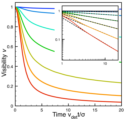
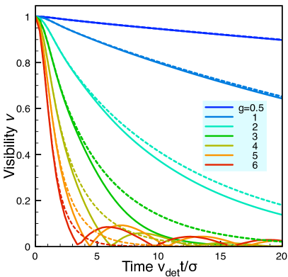
Figure 2: Time-evolution of the visibility (coherence) $v=|D(t)|$ of a qubit coupled to quantum noise from a non-interacting 1D electron channel, at zero temperature, after switching on the interaction at $t=0$. The curves have been obtained by direct numerical evaluation of (19). Left: Decoherence by equilibrium noise, for increasing coupling strength $g$ (top to bottom curve), displaying the power-law decay (33) expected from the physics of the orthogonality catastrophe (inset: log-log plot, with dashed lines indicating the expected exponents $(g/2\pi)^{2}$). Right: Decoherence by shot-noise (at a finite voltage $eV\sigma/v_{{\rm det}}=1$). Beyond $g=\pi$, the visibility displays a periodic pattern, with zeroes and coherence revivals, as a result of the non-Gaussian nature of the noise. Dashed lines indicate the Gaussian approximation. The transmission probability of the barrier generating the shot noise equals $\mathcal{T}=1/2$.

In figure 2, we have displayed the time-evolution of the visibility $v=|D(t)|$ as a function of $v_{{\rm det}}t/\sigma$, for different couplings. In equilibrium, the curves derived from the full expression (19) coincide exactly with those obtained from the Gaussian theory (29), as expected. The long-time behaviour is given by the power-law decay (33) arising from the orthogonality catastrophe. However, at finite voltages, with extra dephasing due to shot noise, the Gaussian approximation fails: In general, it tends to overestimate the visibility at longer times and larger couplings (dashed lines in figure 2, right). The most prominent non-Gaussian feature sets in after the coupling $g$ crosses a threshold that is equal to $g=\pi$, as will be explained below: For larger $g$, the visibility displays oscillations, vanishing at certain times (for a barrier with $\mathcal{T}=1/2$) and showing “coherence revivals” in-between these zeroes. The zeroes coincide with phase jumps of $\pi$ in $D(t)$ (see figure 4). We will discuss the locations of these zeroes in more detail below.

Such a behaviour of the visibility can only be explained by invoking non-Gaussian noise. In every Gaussian theory, we can employ $\left\langle e^{i\varphi}\right\rangle=e^{-\left\langle\varphi^{2}\right\rangle/2}\geq 0$, which directly excludes the behaviour found here (regardless of noise spectrum and coupling strength), even though it is still compatible with a non-monotonous evolution of the visibility. The simplest available model of dephasing by non-Gaussian noise will compared with the present results in section 4.

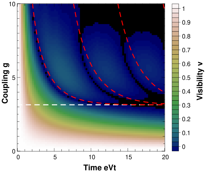
Figure 3: Evolution of the visibility (density plot) as a function of coupling constant $g$ (vertical) and time $eVt$ (horizontal). Visibility oscillations start beyond $g=\pi$. Note the unequal spacing between zeroes: The first zero occurs at a time $eVt_{1}=2\pi^{2}/g$ for large $g\gg 1$, see (42). The spacing of subsequent zeroes is given approximately by $\delta(eVt)=2\pi$ for the regime of couplings considered here. Further parameters: $\mathcal{T}=1/2$ and $eV\sigma/v_{{\rm det}}=1$. The red dashed lines indicate the expected location of visibility zeroes, according to the approximation $v^{\prime}(t)$ for the nonequilibrium part, (37), in the limit $\sigma\rightarrow 0$.

In order to obtain insight into the general structure of the solution, we first of all note that the qualitative features (in particular the zeroes of the visibility) depend only weakly on the width $\sigma$ or shape of the interaction potential. In fact, these features are due to the non-equilibrium part of the noise, and the Gaussian approximation suggests that the limit $\sigma\rightarrow 0$ is well-defined for that part. This is the reason why, in the following, we will plot the time-evolution as a function of $eVt$ (instead of $v_{{\rm det}}t/\sigma$), which is the relevant variable.

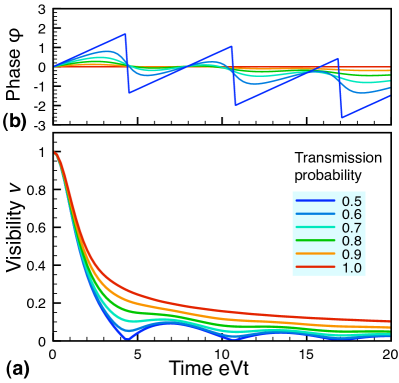
Figure 4: Effect of the transmission probability and phase evolution. (a) Visibility $v=|D(t)|$ as a function of time for different transmission probabilities $\mathcal{T}$ (where $g=5$ and $eV\sigma/v_{{\rm det}}=1$). (b) Corresponding evolution of the phase, i.e. the argument of the complex coherence factor $D_{r}(t)$, where the subscript indicates that the phase evolution for $\mathcal{T}=1$ has been subtracted as a reference.

In figure 3, we display the time-evolution versus the coupling $g$. The threshold at $g=\pi$ is clearly noted. Furthermore, the first zero occurs at a time $t_{1}=2\pi^{2}/(eVg)$ which shrinks with increasing coupling (provided $g\gg 1$, see discussion in the next section and equation (42)). In contrast, subsequent zeroes have a periodic spacing that appears to be roughly independent of $g$, given approximately by $\delta(eVt)=2\pi$ for the small values of $g$ plotted here.

Finally, in figure 4, the effects of the transmission probability $\mathcal{T}$ on the evolution of the visibility and the full coherence factor $D(t)$ have been plotted, indicating the phase jumps obtained at $\mathcal{T}=1/2$ whenever $v=|D(t)|$ vanishes.

All of these features will now be analyzed further by restricting the discussion to the effects of the nonequilibrium part of the noise.

3 Nonequilibrium part of the noise

3.1 General properties

Within the Gaussian approximation, we noted that the visibility at finite voltages factorized into one factor describing the decay due to equilibrium noise and another part describing the effect of nonequilibrium shot noise (34). More precisely, the nonequilibrium part of the visibility can be calculated from (29) by simply restricting the matrix elements of $w_{k^{\prime}k}$ to transitions within the voltage window: $k,k^{\prime}\in[0,eV/v_{{\rm det}}]$. This has the physical interpretation that only these transitions contibute to the excess noise in the spectrum $\left\langle\delta\hat{V}\delta\hat{V}\right\rangle_{\omega}$ of the fluctuating potential. In addition, since the equilibrium noise comes out exact in the Gaussian theory, we can state that all the non-Gaussian features are due to the nonequilibrium part.

Based on these observations, we now introduce a heuristic approximation to the full non-Gaussian theory, which works surprisingly well. We will factorize

$$v^{T=0,V\neq 0}(t)\approx v^{T=V=0}(t)\cdot v^{\prime}(t),$$ (36)

where $v^{\prime}$ is the visibility obtained from the full expression (19) after restricting the matrix elements of $\hat{w}$ in the fashion described above. We will denote the restricted matrix as $\hat{w}^{\prime}$. Note that the restricted matrix depends on the voltage, in contrast to $\hat{w}$ itself.

Since the occupation probability is constant within the voltage window, $n_{k}=\mathcal{T}$, the matrices $\hat{n}$ and $\hat{w}^{\prime}$ now commute. This allows a considerable simplification, yielding a visibility that can be written in terms of the eigenvalues $\varphi_{j}$ of the matrix $\hat{w}^{\prime}$:

$$v^{\prime}(t)=\Pi_{j}|\mathcal{R}+\mathcal{T}e^{-i\varphi_{j}}|.$$ (37)

Thus, the dependence on the transmission probability has been separated from the dependence on interaction potential, time, and voltage, contained within $\varphi_{j}$. The results obtained from the exact formula are compared against this approximation in figure 5 (a). We observe that all the important qualitative features are retained in the approximation. Furthermore, the locations of the zeroes come out quite well, while the amplitude of the oscillations is underestimated.

We will now list some general properties of the matrix $\hat{w}^{\prime}$ that determines the visibility according to (37):
(i) The sum of eigenvalues is

$$\sum_{j}\varphi_{j}={\rm tr}\hat{w}^{\prime}=\frac{g}{2\pi}eVt.$$ (38)

(ii) For a non-negative (non-positive) phase function $w(x)$, the matrix $\hat{w}^{\prime}$ is positive (negative) semidefinite: We can map any wavefunction $\left|\psi\right\rangle$ to another state $\left|\psi^{\prime}\right\rangle$ by setting $\psi^{\prime}_{k}=\psi_{k}$ only inside the voltage window, and $\psi^{\prime}_{k}=0$ otherwise. Then

$$\left\langle\psi\left|\hat{w}^{\prime}\right|\psi\right\rangle=\left\langle\psi^{\prime}\left|\hat{w}\right|\psi^{\prime}\right\rangle=\int dx\,|\psi^{\prime}(x)|^{2}w(x)\geq 0,$$ (39)

for a non-negative function $w(x)$, and analogously for a non-positive function $w(x)$.
(iii) Following the same argument, we can prove that the largest eigenvalue of $\hat{w}^{\prime}$ is bounded by the maximum of $w(x)$, if ${\rm max}w(x)\geq 0$:

$$\left\langle\psi\left|\hat{w}^{\prime}\right|\psi\right\rangle=\int dx\,|\psi^{\prime}(x)|^{2}w(x)\leq\left\langle\psi^{\prime}|\psi^{\prime}\right\rangle{\rm max}w(x)\leq{\rm max}w(x).$$ (40)

Analogously the smallest eigenvalue is bounded from below by the minimum (if ${\rm max}w(x)\leq 0$).

At small voltages (short times) (where $eVt\ll 1$ and $eV\sigma/v_{{\rm det}}\ll 1$), the matrix elements are constant inside the voltage window, $w^{\prime}_{k^{\prime}k}=\frac{1}{L}\tilde{w}(q=0)$, yielding only one nonvanishing eigenvalue, given by (38):

$$\varphi_{1}=\frac{g}{2\pi}eVt\,.$$ (41)

As a consequence, at sufficiently large $g\gg 1$, the first zero in the visibility $v^{\prime}(t)$ will occur when $\varphi_{1}=\pi$, implying

$$t_{1}=\frac{2\pi^{2}}{geV}.$$ (42)

Assuming now that $w(x)$ is non-negative (as is the case in our example, if $g>0$), we can immediately deduce the following general consequences from properties (i) to (iii): All of them taken together imply that the rise of the first eigenvalue must saturate below ${\rm max}w(x)$ (which approaches $g$ for times $v_{{\rm det}}t\gg\sigma$). Thus, other eigenvalues must start to grow, in order to obey the sum-rule. If (and only if) the coupling constant is large enough, this may lead to an infinite series of zeroes in the visibility (see below). Therefore, we are dealing with a true strong coupling effect.

We have not found an analytical way of obtaining $\varphi_{j}$ at arbitrary parameters. However, all relevant features follow from the foregoing discussion and may be illustrated by numerical evaluation of the eigenvalues.

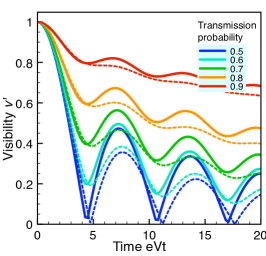
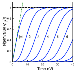
Figure 5: Left: Contribution $v^{\prime}$ of the nonequilibrium part of the noise (i.e. the shot noise) to the suppression of the visibility. The full lines have been obtained from the exact result (19) by dividing by the result at zero voltage, $v^{V\neq 0}(t)/v^{V=0}(t)$. The dashed lines represent the approximation of restricting matrix elements of $\hat{w}$ to the voltage window, see (37). We have set $eV\sigma/v_{{\rm det}}=1$ in this panel. Middle: Universal curves for the eigenvalues $\varphi_{j}$ of the restricted matrix $\hat{w}^{\prime}$ entering the visibility $v^{\prime}(t)$ in equation (37), plotted as a function of $eVt$ in the limit $\sigma\rightarrow 0$. Right: Locations of the zeroes in the visibility $v^{\prime}(t)$ as a function of coupling $g$ (compare figures 3 and 6). These curves can be obtained from those on the left by taking $(2n+1)\pi/(\varphi_{j}/g)$, with $n=0,1,2,3,4,\ldots$ (from bottom to top). The blue dotted line corresponds to the first curve displaced by $2\pi$, indicating the periodicity observed for small couplings $g$. In both panels, the green dashed line shows the short-time behaviour $\varphi_{1}=geVt/2\pi$.

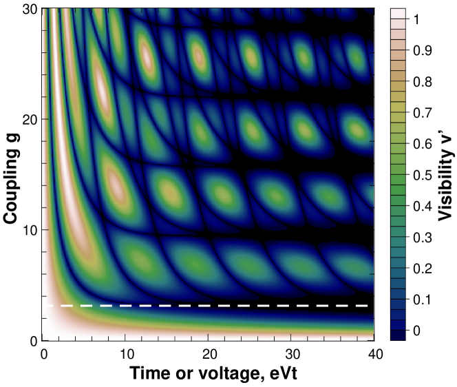
Figure 6: Nonequilibrium part of the visibility, $v^{\prime}$, as a function of coupling strength $g$ and time (or voltage) $eVt$. The lines of vanishing $v^{\prime}$ are those plotted in figure 5. The structure will be distorted for $\sigma>0$, and the full visibility $v$ will be further suppressed at higher couplings by the dephasing due to equilibrium noise, see (36).

We note that the limit $\sigma\rightarrow 0$ is well-defined, and we will assume this limit in the following, in which results become independent of the shape of the interaction potential. This limit represents a good approximation as soon as the time is sufficiently large: $v_{{\rm det}}t\gg\sigma$. In that limit, the eigenvalues have the following functional dependence:

$$\varphi_{j}=g\cdot\varphi_{j}^{(g=1)}(eVt).$$ (43)

Thus the complete behaviour at all coupling strengths can be inferred by numerically evaluating the eigenvalues once as a function of $eVt$. This has been done in figure 6.

At $\mathcal{T}=1/2$, the visibility $v^{\prime}(t)$ will vanish whenever one of these eigenvalues is equal to $(2n+1)\pi$, where $n=0,1,2,\ldots$. Thus, the locations of the zeroes can be obtained from the equation $(2n+1)\pi=\varphi_{j}$, or equivalently $g=(2n+1)\pi/\varphi_{j}^{(g=1)}$. The latter equation has the advantage that the rhs is independent of $g$. It has been used in the right panel of figure 6. These curves have also been inserted into figure 3, for comparison against the results from the full theory. In particular, the first zero is reproduced very accurately, while there are some quantitative deviations at subsequent zeroes.

The full pattern of the visibility, as a function of interaction time and coupling strength, can become very complex due to the large number of lines of vanishing visibility $v^{\prime}$. This is depicted in figure 6.

The analysis in the next section indicates (and the numerical results displayed in figure 6 confirm) that the spacing between the subsequent zeroes in the visibility is no longer determined by $g$, but rather given by $2\pi/eV$ (with deviations at higher $g$). As we will explain in the next section, this corresponds to one additional detector electron passing by the qubit during the interaction time.

3.2 Wave packet picture

Following Martin and Landauer [47], we introduce a new basis of states inside the voltage window, whose width in k-space is set by $\Delta k\equiv eV/v_{{\rm det}}$:

$$\left|\psi_{n}\right\rangle=\left(\frac{\Delta k}{2\pi/L}\right)^{-1/2}\sum_{k\in[0,\Delta k]}e^{-ikn\Delta x}\left|k\right\rangle.$$ (44)

In real space, these states represent a train of wavepackets, spaced apart by $\Delta x=2\pi/\Delta k=v_{{\rm det}}\Delta t$, corresponding to time bins of duration $\Delta t=h/eV=2\pi/eV$. Taking the limit $L\rightarrow\infty$, we have

$$\psi_{n}(x)=\sqrt{\frac{\Delta k}{2\pi}}e^{i\frac{\Delta k}{2}(x-n\Delta x)}{\rm sinc}(\frac{\Delta k}{2}(x-n\Delta x)),$$ (45)

where ${\rm sinc}(y)=\sin(y)/y$. These packets move at constant velocity, $\psi_{n}(x,t)=\psi_{n}(x-v_{{\rm det}}t)$. Their advantage is that they are localized in space and therefore well suited for calculating matrix elements of the phase function $w(x)$ (or its restricted counterpart $\hat{w}^{\prime}$). From

$$\left\langle\psi_{n^{\prime}}\left|\hat{w}\right|\psi_{n}\right\rangle=\left(\frac{\Delta k}{2\pi/L}\right)^{-1}\sum_{k,k^{\prime}\in[0,\Delta k]}e^{i(k^{\prime}n^{\prime}-kn)\Delta x}w_{k^{\prime}k}$$ (46)

we find

$$\left\langle\psi_{n^{\prime}}\left|\hat{w}\right|\psi_{n}\right\rangle=\frac{\Delta k}{2\pi}\int_{-1}^{+1}d\tilde{q}\,e^{i\pi(n+n^{\prime})\tilde{q}}G_{n^{\prime}-n}(|\tilde{q}|)\tilde{w}(\tilde{q}\Delta k),$$ (47)

where

$$G_{n^{\prime}-n}(|\tilde{q}|)=\left\{\begin{array}[]{c}\frac{\sin(\pi|\tilde{q}|(n^{\prime}-n))}{\pi(n-n^{\prime})}\,\,{\rm for}\,n^{\prime}\neq n\\ 1-|\tilde{q}|\,\,{\rm for}\,n^{\prime}=n\end{array}\right..$$ (48)

These formulas enable a very efficient numerical evaluation. In general, for large $|n|$ and $|n^{\prime}|$ the corresponding wave packets lie outside the range of $w(x)$ and therefore the corresponding matrix elements are small and can be neglected. In the limit of small voltages, the matrix $\hat{w}^{\prime}$ is already diagonal in this basis (compare (41)):

$$\left\langle\psi_{n^{\prime}}\left|\hat{w}\right|\psi_{n}\right\rangle\approx\left[\frac{geVt}{2\pi}\right]\delta_{n^{\prime}0}\delta_{n0}.$$ (49)

Moreover, the wave packet basis permits a very intuitive interpretation of the results in the Gaussian approximation: First, let us assume that the number of contributing wave packets is large, $N\equiv eVt/2\pi\gg 1$. The wave packets are orthonormalized, and the phase function $w(x)$ is smooth on the scale $\Delta x=v_{{\rm det}}\Delta t=v2\pi/eV$ of these packets (for sufficiently large voltages). As a result, we find that the matrix $\hat{w}$ is diagonal in this basis, up to terms of order $1/N$:

$$\left\langle\psi_{n^{\prime}}\left|\hat{w}\right|\psi_{n}\right\rangle\approx\delta_{n^{\prime}n}w(x=n\Delta x)+O\left(\frac{1}{N}\right).$$ (50)

Therefore, in any sum over the eigenvalues $\varphi_{j}$, these can be approximated by the values of $w$ taken at the centers of the wave packets. Assuming further that the coupling $g\ll 1$ is weak, each of the $\varphi_{j}$ is small. This allows us to expand the visibility reduction due to nonequilibrium noise:

$$v^{\prime}(t)=\Pi_{j}|\mathcal{R}+\mathcal{T}e^{-i\varphi_{j}}|\approx 1-\frac{1}{2}\mathcal{RT}\sum_{j}\varphi_{j}^{2}+\ldots$$ (51)

That is the expected result, which has the form of “phase diffusion”, with a contribution from the variance of the phase shift exerted by each detector electron. In the limit of $\sigma\ll eVt$, we get $\varphi_{j}=g$ for approximately $N$ wave packets, and zero otherwise. Then we reproduce equation (35) in the long-time limit:

$$\sum_{j}\varphi_{j}^{2}=Ng^{2}=\frac{t}{\Delta t}g^{2}=\frac{eVt}{2\pi}g^{2}.$$ (52)

More generally, for any shape of $w(x)$ we can replace

$$\sum_{j}\varphi_{j}^{2}\approx\sum_{n}\left\langle\psi_{n}\left|\hat{w}\right|\psi_{n}\right\rangle^{2}\approx\frac{1}{\Delta x}\int dx\,w^{2}(x).$$ (53)

Defining the effective width of $w(x)$ as

$$l_{{\rm eff}}\equiv\frac{\left[\int dx\,w(x)\right]^{2}}{\int dx\,w^{2}(x)},$$ (54)

we can set the total number of wave packets to be $N=l_{{\rm eff}}/\Delta x$. Defining the average phase shift induced by a single detector electron as $\bar{\varphi}=\int dx\,w(x)/(N\Delta x)=(geVt/2\pi)/N$, we can write

$$\sum_{j}\varphi_{j}^{2}\approx N\bar{\varphi}^{2}.$$ (55)

Note that in the case of a constant $w(x)$, we have $l_{{\rm eff}}=v_{{\rm det}}t$, and therefore $N=eVt$ and $\bar{\varphi}=g$, so we are back to (52).

4 Comparison with dephasing by classical telegraph noise

In this section, we compare and contrast the results we have obtained in the rest of this paper against the simplest possible model displaying non-Gaussian features in dephasing: pure dephasing of a qubit by classical random telegraph noise. There, visibility oscillations are observed once the coupling strength becomes large as compared to the switching rate of the two-state fluctuator producing the telegraph noise. In the limit of a vanishing switching rate, the visibility in that model is the average of two oscillatory phase factors evolving at different frequencies, corresponding to the two different energy shifts imparted by the two-state fluctuator:

$$v^{{\rm tel.noise}}(t)=|(1-p)+pe^{-i\delta\omega t}|.$$ (56)

If the occupation probability of the two fluctuator states is $p=1/2$, this leads to visibility oscillations $v^{{\rm tel.noise}}(t)=\left|\cos(\delta\omega t)\right|$, roughly similar to those found in our full quantum theory of dephasing by shot noise. The decaying envelope of these oscillations is then produced by a finite switching probability.

It is instructive to set up a rough correspondence between that simple model and the one considered here, and see how far it takes us (and where it fails): According to the well-known semiclassical picture of binomial shot noise [30], during the time-interval $\Delta t=h/eV=2\pi/eV$ a single detector electron arrives with a probability $\mathcal{T}$. It imparts a phase shift $g$ within our model. Thus, the fluctuator probability $p$ would equal $\mathcal{T}$, the mean time between telegraph noise switching events would be taken as $\Delta t$, and the frequency difference $\delta\omega$ would have to be set equal to $g/\Delta t$. This analogy partly suggests the right qualitative behaviour, namely a threshold in $g$ that is independent of voltage (independent of $\Delta t$). This threshold turns out to be $g=1$ in the telegraph noise model, and for larger $g$ the visibility oscillates with a period $4\pi\Delta t/\sqrt{g^{2}-1}$ (if $p=\mathcal{T}=1/2$). Although this correctly suggests that the first zero occurs at a position $t\propto 1/(eVg)$, it predicts all subsequent zeroes to occur at the same period, which is not compatible with the actual behaviour (see figure 3). These discrepancies are not too surprising, since the two models certainly differ even qualitatively in the following sense: In random telegraph noise, the switching occurs in a Markoff process, i.e. without memory. In contrast, in the semiclassical model of binomial shot noise the electrons arrive in a stream of regularly spaced time-bins of size $\Delta t=h/eV$. We have not found any reasonable way of incorporating this fact into a simplified semiclassical model, since it is unclear how to treat ’fractional time-bins’ within such a model.

5 Electronic Mach-Zehnder interferometer coupled to a detector edge channel

In this section we will show how to explain the surprising experimental results that have been obtained recently in a strongly coupled “which-path detector system” involving a Mach-Zehnder interferometer coupled to a “detector” edge channel. We will present a nonperturbative treatment that captures all the essential features due to the non-Gaussian nature of the detector shot noise. Our approximate solution for this model is directly related to the exact solution of the simpler charge qubit system discussed above.

A simplified scheme of the experimental setup is presented in figure 1 (see [31, 32] for a detailed explanation). Both the MZI and the detector were realized utilizing chiral one-dimensional edge-channels in the integer Quantum Hall effect regime. The MZI phase was controlled by a modulation gate via the Aharonov-Bohm (AB) effect. The additional edge channel was partitioned by a quantum point contact, before traveling in close proximity to the upper path of the MZI, serving as a ”which path” phase-sensitive detector [23]. For a finite bias applied to the detector channel, the Coulomb interaction between both channels caused orbital entanglement between the interfering electron and the detecting electrons, thereby decreasing the contrast of the AB oscillations. This contrast, quantified in terms of the visibility $v=(I_{{\rm max}}-I_{{\rm min}})/(I_{{\rm max}}+I_{{\rm min}})$, was measured as a function of the DC bias $V$ applied at the detector channel, and of the partitioning probability $\mathcal{T}$ of the detector channel.

As noted already in the introduction, two new and peculiar effects, which will be explained here, were observed in these experiments:

• Unexpected dependence on partitioning: The visibility as a function of $\mathcal{T}$ changes from the expected smooth parabolic suppression $\propto\mathcal{T}(1-\mathcal{T})$ at low detector voltages to a sharp “V-shape” behaviour at some larger voltages, with almost zero visibility at $\mathcal{T}=1/2$ (see Fig. 3 in [32]).

• Visibility oscillations: For some values of the detector QPC gate voltage (yielding $\mathcal{T}\approx 1/2$), the visibility drops to zero at intermediate voltages, then reappears again as $V$ increases, in order to vanish at even larger voltages (see Fig. 4 in [32]). For some other gate voltages it decreases monotonically (see Fig. 2 in [31]).

In [32] we showed that a simplified model involving a single detector electron can provide a qualitative explanation for the experimental results listed above. However, it has clear shortcomings, both quantitative and in terms of the physical interpretation. The natural reason for these shortcomings is that detection in the experiment is due to a varying number of electrons, not just a single one. Then two questions arise: (i) How many electrons dephase the MZI as the detector voltage increases, and (ii) how much does each electron contribute to dephasing. These questions will be answered by the following model.

5.1 Solution of the single-particle problem

The main simplifying assumption in our approach will be that it is possible to treat each given electron in the Mach-Zehnder interferometer on its own, as a single particle interacting with the fluctuations of the density in the detector channel. Making this assumption is far from being a trivial step, as it effectively neglects Pauli blocking, and we will have to comment on it in the next section. For now, however, let us define the following model as our starting point:

$$\hat{H}=v_{{\rm MZ}}\hat{p}+\int dx^{\prime}\,u(x^{\prime}-\hat{x})\hat{\rho}_{{\rm det}}(x^{\prime})+\hat{H}_{{\rm det}}.$$ (57)

Here $\hat{x}$ and $\hat{p}=-i\partial_{x}$ are the position and the momentum operator, respectively, of the single interfering electron under consideration (traveling in the upper, interacting path of the interferometer). We have linearized the dispersion relation, keeping in mind that the interferometer’s visibility will be determined by the electrons near the MZ Fermi energy, traveling at a speed $v_{{\rm MZ}}$. The Fermi energy itself has been subtracted as an irrelevant energy offset, and likewise the momentum is measured with respect to the Fermi momentum. The Aharonov-Bohm phase between the interfering paths would have to be added by hand.

We thus realize that the situation is analogous to the model treated above, involving pure dephasing of a charge qubit. The two states of the qubit correspond to the two paths which the interfering electron can take. The following analysis explicitly demonstrates this equivalence and arrives at an expression for the visibility which is the analogue of equation (6). The only difference will be the replacement of $v_{{\rm det}}$ by the relative velocity $v_{{\rm det}}-v_{{\rm MZ}}$, which can be understood by going into the frame of reference of the MZ electron.

Let us now consider the full wave function $\left|\Psi_{{\rm total}}(t)\right\rangle=e^{+i\hat{H}_{{\rm det}}t}e^{-i\hat{H}t}\left|\Psi_{{\rm total}}(0)\right\rangle$ of MZI and detector, expressed in the interaction picture with respect to $\hat{H}_{{\rm det}}$. One can always decompose the full wave function in the form $\left|\Psi_{{\rm total}}(t)\right\rangle=\int dx\,\left|x\right\rangle\otimes\left|\psi(x,t)\right\rangle$. Here, we focus on the projection $\left|\psi(x,t)\right\rangle\equiv\left\langle x\left|\Psi_{{\rm total}}(t)\right.\right\rangle$ onto the MZI single-particle position basis. This is a state in the detector Hilbert space, with $\left\langle\left.\psi(x,t)\right|\psi(x,t)\right\rangle$ giving the probability of the MZI electron to be found at position $x$. It obeys the Schrödinger equation

$$i\frac{\partial}{\partial t}\left|\psi(x,t)\right\rangle=\left[-iv_{{\rm MZ}}\frac{\partial}{\partial x}+\hat{V}(x,t)\right]\left|\psi(x,t)\right\rangle,$$ (58)

where the fluctuating potential $\hat{V}(x,t)\equiv\int dx^{\prime}\,u(x^{\prime}-x)\hat{\rho}_{{\rm det}}(x^{\prime},t)$ is in the interaction picture with respect to $\hat{H}_{{\rm det}}$. The exact solution of equation (58) that follows from the Hamiltonian (57) reads:

$$\left|\psi(x,t)\right\rangle=\hat{T}\exp\left[-i\int_{0}^{t}dt^{\prime}\,\hat{V}(x-v_{{\rm MZ}}t^{\prime},t-t^{\prime})\right]\left|\psi(x-v_{{\rm MZ}}t,0)\right\rangle.$$ (59)

Thus, at a given space-time point $(x,t)$, the “quantum phase” in the exponent is an integral over the values of the fluctuating potential at all points on the “line of influence” $(x^{\prime},t^{\prime})$ with $x-x^{\prime}=v_{{\rm MZ}}(t-t^{\prime})$. If the potential were classical, the exponential would represent a simple phase factor. Here, however, the interfering electron is not only acted upon by the fluctuations but also changes the state of the detector. The state $\left|\psi(x,t)\right\rangle$ contains all the information about the entanglement between the MZI electron and the detector electrons.

We will now determine the visibility resulting from the interaction between interferometer and detector channel. At the first beam splitter, the electron’s wave packet is decomposed into two parts, one of them traveling along the lower ($l$) arm of the interferometer, the other one traveling along the upper ($u$) arm. These are described by states $\left|\psi_{l}(x,t)\right\rangle$ and $\left|\psi_{u}(x,t)\right\rangle$, respectively, which obey the Schrödinger equation given above, albeit in general with a different noise potential for each of them. The visibility is determined by the overlap between those two states, taken at the position $x=v_{{\rm MZ}}t$ of the second beam splitter (where $t$ is the time-of-flight through the interferometer):

$$v=\left|\left\langle\psi_{l}(x,t)|\psi_{u}(x,t)\right\rangle\right|.$$ (60)

Taking into account that $\left|\psi_{l,u}(0,0)\right\rangle=\left|\Psi_{{\rm det}}\right\rangle$ is the detector’s initial unperturbed state, and realizing that the interaction takes place only in the upper arm, we find that the visibility is determined by the probability amplitude for the electron to exit the MZI without having changed the state of the detector [18]:

$$v=\left|\left\langle\Psi_{{\rm det}}\left|\hat{T}\exp\left[-i\int_{0}^{t}dt^{\prime}\,\hat{V}(x-v_{{\rm MZ}}t^{\prime},t-t^{\prime})\right]\right|\Psi_{{\rm det}}\right\rangle\right|.$$ (61)

The initial detector state $\left|\Psi_{{\rm det}}\right\rangle$ itself is produced by partitioning a stream of electrons.

The last step consists in representing equation (61) as an expectation value of a unitary operator:

$$v=\left|\left\langle\Psi_{{\rm det}}\left|e^{-i\hat{\Phi}}\right|\Psi_{{\rm det}}\right\rangle\right|,$$ (62)

where $\hat{\Phi}$ is defined as the operator in the exponent of (61). We have been allowed to drop the time ordering symbol because the density fluctuations in the one-dimensional detector channel are described by free bosons: $\left[\hat{\rho}(x,t),\hat{\rho}(x^{\prime},t^{\prime})\right]$ is a purely imaginary c-number. The time-ordered exponential is by definition a product of many small unitary evolutions sorted by time. Hence, using repeatedly the Baker-Hausdorff formula $e^{\hat{A}}e^{\hat{B}}=e^{\hat{A}+\hat{B}}e^{[\hat{A},\hat{B}]/2}$, which holds since $[\hat{A},\hat{B}]$ commutes with $\hat{A}$ and $\hat{B}$ in this case, we can collect the operators at different times into the same exponent. The remaining c-number exponent only contributes a phase, so it does not lead to a reduction in the visibility and we can disregard it.

The phase operator $\hat{\Phi}$ in (62) is therefore a weighted integral over the density operator:

$$\hat{\Phi}=\int_{0}^{t}dt^{\prime}\hat{V}(x-v_{{\rm MZ}}t^{\prime},t-t^{\prime})=\int dx^{\prime}\,w(x^{\prime})\hat{\rho}_{{\rm det}}(x^{\prime})dx^{\prime}=\sum_{k,k^{\prime}}w_{k^{\prime}k}\hat{d}_{k^{\prime}}^{\dagger}\hat{d}_{k}.$$ (63)

The phase function $w(x)$ is the one that has been introduced before, in equation (18), with the exception that the detector velocity has to be replaced by the relative velocity: $v_{{\rm det}}\mapsto v_{{\rm det}}-v_{{\rm MZ}}$. It can be viewed as a convolution of the interaction potential $u(x)$ with the “window of influence” of length $l=|(v_{{\rm det}}-v_{{\rm MZ}})t|$ defined by the traversal time $t$ and the velocities.

5.2 Approximate treatment of Pauli blocking

The loss of visibility is due to the trace a particle leaves in the detector [18]. If the detector (or, in general, the environment) is in its ground state initially, this means that the detector has to be left in an excited state afterwards. Energy conservation implies that the energy has to be supplied by the particle itself. This is no problem if the particle starts out in an excited state. An example is provided by a qubit in a superposition of ground and excited state, which can decay to its ground state by spontaneous emission of radiation into a zero-temperature environment.

However, in electronic interference experiments such as the one considered here, we are interested in the loss of visibility with regard to the interference pattern observed in the linear conductance. At zero temperature, this implies we are dealing with electrons right at the Fermi surface which have no phase space available for decay into lower-energy states, due to Pauli blocking. Only an environment that is itself in a nonequilibrium state (e.g. the voltage-biased detector channel) can then lead to dephasing. This very basic physical picture has been confirmed by many different calculations. While it is, in principle, conceivable that subtle non-perturbative effects might eventually lead to a break-down of this picture, we are not aware of any unambiguous and uncontroversial theoretical derivation of a suppression of linear conductance visibility at zero temperature, for an interferometer coupled to an equilibrium quantum bath.

The main difficulty in dealing with an electronic interferometer coupled to a quantum bath thus lies in the necessity of treating the full many-body problem. Any model that considers only a single interfering particle subject to the environment will miss the effects of Pauli blocking, and thereby permit unphysical, artificial dephasing by spontaneous emission events that would be absent in a full treatment. In [38, 40], it was shown how to properly incorporate these effects into an equations-of-motion approach similar to the one described above (with the fermion field $\hat{\psi}(x,t)$ taking the role of the single-particle state $\left|\psi(x,t)\right\rangle$). The main idea was that the state of the detector, and therefore the noise potential $\hat{V}$, will itself be influenced by the density in the interferometer, leading to “backaction terms” (known from the quantum Langevin equation for quantum dissipative systems) that ultimately ensure Pauli blocking. However, in order to be able to solve the equations of motion of the environment, it was crucial to assume Gaussian quantum noise, and even then the solution for the visibility was carried out only to lowest order in the coupling. Thus, this approach is not feasible for the present problem, where we want to keep non-Gaussian effects in a fully nonperturbative way. Nevertheless, the underlying intuitive physical picture remains valid: If both the interferometer and the detector are near their ground states, the interfering electron will get “dressed” by distorting the detector electron density in its vicinity, but this perturbation is undone when it leaves the interaction region. Therefore no trace is left and there is no contribution to the dephasing rate.

We therefore resort to an approximate treatment (applicable to the zero-temperature situation), suggested by the general physical picture described above. We will continue to use the single-particle picture for the interferometer, but keep only the nonequilibrium part of the noise, thus eliminating the possibility of artificial dephasing for the case when the detector is not biased. In fact, within a lowest-order perturbative calculation, this scheme gives exactly the right answers: Firstly, dephasing by the quantum equilibrium noise of the detector channel is completely eliminated by Pauli blocking, as follows from the analysis of [38, 40] (at $T=0$, for the linear conductance). Secondly, the remaining nonequilibrium part of the noise spectrum, corresponding to the shot noise, is symmetric in frequency, and thus equivalent to purely classical noise whose effects are not diminished by Pauli blocking (see discussions in [40, 48]).

The analysis in section 3.1 has demonstrated that all the non-Gaussian features are due to the nonequilibrium part which we retain. Therefore, we expect that the present approximation should be able to reproduce the novel features observed in the experiment, which is confirmed by comparison with the experimental data. We emphasize once more that it is crucial to supplement the single-particle picture by taking care of the Pauli principle afterwards.

Thus, we shall restrict the matrix elements in equation (63) to the voltage window, replacing $w_{k^{\prime}k}$ by the restricted $w^{\prime}_{k^{\prime}k}$, according to the notation introduced in section 3.1. All that remains to be done to calculate the visibility is diagonalizing the operator $\hat{\Phi}$, which is achieved by switching to the basis of eigenstates of $w^{\prime}$,

$$\hat{\Phi}=\sum_{j}\varphi_{j}\hat{c}_{j}^{\dagger}\hat{c}_{j},$$ (64)

where $\varphi_{j}$ are the eigenvalues and $\hat{c}_{j}$ is the annihilation operator for eigenstate $j$ of $w^{\prime}$. The occupation operators $\hat{c}_{j}^{\dagger}\hat{c}_{j}$ fluctuate independently, and all states $j$ have the same occupation probability $\mathcal{T}$, just like the states in the original basis. This is a consequence of the occupation matrix being proportional to the identity matrix, as pointed out near equation (37). Therefore, equation (63) reduces to

$$v^{\prime}=\left|\left\langle e^{-i\hat{\Phi}}\right\rangle\right|=\left|\left\langle\Psi_{{\rm det}}\left|\Pi_{j}e^{-i\varphi_{j}\hat{c}_{j}^{\dagger}\hat{c}_{j}}\right|\Psi_{{\rm det}}\right\rangle\right|=\Pi_{j}\left|\mathcal{R}+\mathcal{T}e^{-i\varphi_{j}}\right|.$$ (65)

This formula is our main result for the visibility of the MZI, valid at zero temperature. It gives a closed expression for the reduction of the interference contrast in the AB oscillations of the MZI, as a function of detector bias and partitioning probability $\mathcal{T}$. It has been calculated nonperturbatively within the approximation discussed above, i.e. employing a single-particle picture for the interfering electron and simultaneously retaining only the nonequilibrium part of the detector noise. At any given detector voltage $V$, there exists a basis of states in the detector, which, when occupied, contribute to the MZI phase by different amounts $\varphi_{j}$. These occupations fluctuate due to the partitioning at the detector beam splitter. The visibility then is the product of all those influences.

5.3 Dependence of visibility on detector voltage and detector partitioning

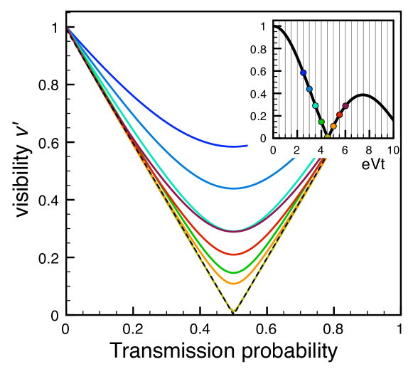
Figure 7: Dependence of the visibility $v^{\prime}$ on the partitioning probability $\mathcal{T}$ of the detector current, for different voltages, using equation (65). The “V-shape” is clearly observed. Inset: Visibility at $\mathcal{T}=1/2$ as a function of $eVt$. The locations corresponding to the curves in the main plot are indicated. Other parameters: $g=5$ and temperature $T=0$.

The visibility for the Mach-Zehnder interferometer subject to the shot noise in the detector channel may thus be calculated in the same manner as the visibility for the charge qubit treated above, if the restriction to the nonequilibrium part of the noise is taken into account. The main difference is that in the MZI the interaction time $t$ is dictated by the setup. However, in the limit $\sigma\rightarrow 0$, the visibility $v^{\prime}$ only depends on the product $eVt$. Thus the plots above (figures 5 (b,c) and 6) also depict the dependence of $v^{\prime}$ on the voltage at fixed time $t$.

At small bias voltages, only one eigenvalue is nonzero and grows linearly with detector voltage, according to equation (41): $\varphi_{1}=geVt/2\pi\equiv\gamma V$. Thus, the visibility is

$$v^{\prime}=|\mathcal{R}+\mathcal{T}e^{-i\gamma V}|,$$ (66)

where the proportionality constant $\gamma$ may be measured from the voltage-dependent phase shift obtained for the non-partitioned case, $\mathcal{T}=1$. Equation (66) represents the influence of “exactly one detecting electron”.

One can obtain (66) as an ansatz, by postulating that exactly one detector electron interacts with the interfering electron [32]. Here we obtained it naturally as a limiting case of our full expression. It has to be emphasized that this result is highly counterintuitive: Naively, one would assume that each detector electron induces a constant phase shift that is set by the coupling strength and does not depend on the detector voltage. The voltage $V$ should only control the frequency at which detector electrons are injected. However, to the extent that we identify each eigenvalue $\varphi_{j}$ with one detector electron, we have to conclude that this naive picture is wrong. Formally, only a single, very extended detector wavepacket of size $\propto V^{-1}$ interacts with the quantum system, i.e. the charge qubit or the interfering electron (see section 3.2). As the interaction range is fixed and limited, this means that the phase shift (basically the expectation value of $w(x)$ in terms of this wave packet) then shrinks with $V$. The linear dependence of the phase shift on voltage thus may be rationalized by taking into account energy conservation: At lower detector voltages $V$ the phase space for scattering of detector electrons gets restricted severely, and thus the effective interaction strength is diminished. Likewise, the spatial resolution of this which-path detector becomes very poor, as is apparent from the large extent of the wave packet: Detection at a high spatial resolution would prepare a localized state that contains a lot of energy, more than is available in the detector-interferometer system.

Regarding the dependence on the transmission probability of the detector channel (figure 7), we note that there are strong deviations from the smooth dependence $\exp[-{\rm C}\mathcal{T}(1-\mathcal{T})]$ expected for any Gaussian noise model (where $C$ would depend on $V,t,g,\ldots$ but not on $\mathcal{T}$). These deviations are particularly strong near the voltages for which the visibility becomes zero at $\mathcal{T}=1/2$. Indeed, if only one eigenvalue contributes and is equal to $\pi$, equation (66) yields a “V-shape” of the visibility, $v^{\prime}=|1-2\mathcal{T}|$, as indicated by the dashed line in figure 7.

5.4 Comparison with experiment

In this section we briefly discuss the results obtained by fitting the present model to the experimental data. This follows our discussion in [32], where the reader may find the relevant figures.

At the outset, we note that the visibility in the real experiment is also suppressed by external low-frequency fluctuations, beyond the detector-induced dephasing discussed here. They contribute an overall voltage-independent factor that has to be introduced as a fitting parameter when comparing against theory.

First, we consider the approximation (66) obtained for low voltages, involving only one detector electron. Since the constant $\gamma$ was measured, this formula does not contain any free parameters, and can be compared directly with the experimental data. As shown in Fig. 3 of [32], it fits very well to the data at low $V$ and qualitatively reproduces the novel effects mentioned at the beginning of section 5. In particular, it predicts the change from a smooth shape to a V-shape in the dependence of visibility on partitioning probability, as well as the non-monotonous behaviour with increasing $V$. However, according to (66) these effects should occur when $\gamma V=\pi$, which does not agree with the experimental observations, where the zero in the visibility is shifted to a detector bias that is larger than this estimate by about 40%. Hence at this detector bias (66) fails to quantitatively reproduce the experimental results. The reason of this discrepancy must be the onset of the contributions from other detecting electrons. Once other eigenvalues become slightly non-zero, the first one is smaller than $\gamma V$, because of the sum rule (38) and the non-negativity of the eigenvalues, (39). This is clearly apparent in figure 6. The visibility then vanishes at larger values of the detector voltage $V$, in agreement with experiment. At even larger voltages, near $\varphi_{1}\approx 2\pi$, the visibility will have again a maximum (coherence revival). However, it will be smaller due to the dephasing by the other detecting states (other $\varphi_{j}$), again in contrast to the simplified formula (66). These two effects have both been seen in the experiment (Fig. 4 in [32]).

Finally, in [32], we fitted the experimental data by using, for simplicity, a Lorentzian shape as an ansatz for the Fourier transform of the phase function:

$$\tilde{w}(q)=\frac{\tilde{w}(q=0)}{1+\left(\frac{qv_{{\rm det}}}{eV_{*}}\right)^{2}}$$ (67)

Here $V_{*}$ has the dimensions of a voltage and turns out to be $V_{*}\approx 6.2\,\mu V$. Within this fit, the first eigenvalue is $\varphi_{1}\approx 0.8\pi$ at $V=9.5\mu V$, where $\gamma V=\pi$. This implies that almost the full phase shift of $\pi$ is contributed by a single electron, indicating very strong interchannel interaction.

5.5 Relation to intrinsic visibility oscillations

While the earliest implementation of the electronic MZI [22] displayed a rather smooth monotonous decay of the visibility with rising MZI bias voltage, this is no longer true in a more recent version [34]. There, the visibility displayed oscillations, much like the ones observed here, except they occured as a function of MZI bias voltage, in the absence of any detector channel. The present analysis may lead to a possible explanation for these initially puzzling observations: The intrinsic intra-channel interaction may cause the interfering electrons to be dephased by their own (non-Gaussian) shot noise, if the bias is large enough. We note that a similar explanation was put forward in a recent preprint of Sukhorukov and Cheianov [42], who considered a model where two counterpropagating edge channels interacted with each other. Though their model is therefore different from ours, we have seen that the visibility oscillations are a generic consequence of dephasing by non-Gaussian shot noise, and therefore it is hard to distinguish experimentally (at this point) between the different models.

6 Summary and conclusions

We presented a nonperturbative approach to the dephasing of a quantum system by an adjacent partitioned one-dimensional electron channel, serving as a detector. Our treatment gave an exact expression for the time-evolution of the visibility of a charge qubit coupled to such a detector. Moreover, within a certain simplifying approximation, it can be used to describe a “controlled dephasing” (or “which path”) setup where a Mach-Zehnder interferometer is coupled to a detector channel.

The main features of our results are the following: The visibility may display oscillations as a function of time or detector voltage, vanishing exactly at certain points and yielding “coherence revivals” in-between those points. This behaviour is only observed if the coupling strength crosses a certain voltage-independent threshold, corresponding to a phase-shift of $g=\pi$ contributed by a single electron. It is impossible to obtain that behaviour in any model of dephasing by Gaussian noise, regardless of the assumed noise spectrum. The location of the first zero of the visibility (in detector voltage or interaction time) is proportional to $1/g$ for large couplings $g$, while the spacing of subsequent zeroes is approximately independent of $g$ and corresponds to injecting one additional detector electron during the interaction time. When plotted as a function of detector transmission probability, the visibility differs from the smooth dependence on $\mathcal{T}(1-\mathcal{T})$ expected for any Gaussian model, rather displaying a “V-shape” at certain voltages.

All of these features have been observed in the recent Mach-Zehnder experiment [32]. Challenges for future experiments include more quantitative comparisons against the theory presented here, as well as finding ways of tuning the interaction strength $g$, to switch between the strong and weak coupling regimes. In addition, we hope that the strong coupling physics of dephasing by non-Gaussian shot noise will be seen in future experiments involving various other kinds of quantum systems as well.

Acknowledgements. - We thank B. Abel, L. Glazman, D. Maslov, M. Büttiker, Y. Levinson, D. Rohrlich, and M. Heiblum for fruitful discussions. This work was partly supported by the Israeli Science Foundation (ISF), the Minerva foundation, the German Israeli Foundation (GIF), the SFB 631 of the DFG, and the German Israeli Project cooperation (DIP).

References

- [1] A. O. Caldeira and A. J. Leggett. Influence of dissipation on quantum tunneling in macroscopic systems. Phys. Rev. Lett., 46:211, 1981.
- [2] A. O. Caldeira and A. J. Leggett. Path integral approach to quantum brownian motion. Physica, 121A:587, 1983.
- [3] A. J. Leggett, S. Chakravarty, A. T. Dorsey, M. P. A. Fisher, A. Garg, and W. Zwerger. Dynamics of the dissipative two-state system. Rev. Mod. Phys., 59:1, 1987.
- [4] U. Weiss. Quantum Dissipative Systems. World Scientific, Singapore, 2000.
- [5] E. Paladino, L. Faoro, G. Falci, and R. Fazio. Decoherence and 1/f noise in josephson qubits. Phys. Rev. Lett., 88:228304, 2002.
- [6] H Gassmann, F Marquardt, and C Bruder. Non-Markoffian effects of a simple nonlinear bath. Phys. Rev. E, 66:041111, 2002.
- [7] Y. Makhlin and A. Shnirman. Dephasing of solid-state qubits at optimal points. Phys. Rev. Lett., 92:178301, 2004.
- [8] R. W. Simmonds et al. Decoherence in Josephson phase qubits from junction resonators. Phys. Rev. Lett., 93:077003, 2004.
- [9] O. Astafiev, Yu. A. Pashkin, Y. Nakamura, T. Yamamoto, and J. S. Tsai. Quantum noise in the Josephson charge qubit. Phys. Rev. Lett., 93:267007, 2004.
- [10] A. Grishin, I. V. Yurkevich, and I. V. Lerner. Low-temperature decoherence of qubit coupled to background charges. Phys. Rev. B, 72:060509(R), 2005.
- [11] G. Ithier et al. Decoherence in a superconducting quantum bit circuit. Phys. Rev. B, 72:134519, 2005.
- [12] R. de Sousa, K. B. Whaley, F. K. Wilhelm, and J. v. Delft. Ohmic and step noise from a single trapping center hybridized with a Fermi sea. Phys. Rev. Lett., 95:247006, 2005.
- [13] J. Schriefl, Y. Makhlin, A. Shnirman, and G. Schön. Decoherence from ensembles of two-level fluctuators. New Journal of Physics, 8:1, 2006.
- [14] Y. M. Galperin, B. L. Altshuler, J. Bergli, and D. V. Shantsev. Non-gaussian low-frequency noise as a source of qubit decoherence. Phys. Rev. Lett., 96:097009, 2006.
- [15] V. B. Braginsky and F. Y. Khalili. Quantum Measurement. Cambridge University Press, Cambridge, 1992.
- [16] A. A. Clerk, S. M. Girvin, and A. D. Stone. Quantum-limited measurement and information in mesoscopic detectors. Phys. Rev. B, 67:165324, 2003.
- [17] U. Gavish, B. Yurke, and Y. Imry. Generalized constraints on quantum amplification. Phys. Rev. Lett., 93:250601, 2004.
- [18] A. Stern, Y. Aharonov, and Y. Imry. Phase uncertainty and loss of interference: A general picture. Phys. Rev. A, 41:3436, 1990.
- [19] Y. Imry. Introduction to Mesoscopic Physics. Oxford University Press, 2 edition, 2002.
- [20] Y. Levinson. Dephasing in a quantum dot due to coupling with a quantum point contact. Europhysics Letters, 39:299, 1997.
- [21] I. L. Aleiner, N. S. Wingreen, and Y. Meir. Dephasing and the orthogonality catastrophe in tunneling through a quantum dot: The ”which path?” interferometer. Phys. Rev. Lett., 79:3740, 1997.
- [22] E. Buks, R. Schuster, M. Heiblum, D. Mahalu, and V. Umansky. Dephasing in electron interference by a ”which-path” detector. Nature, 391:871, 1998.
- [23] D. Sprinzak, E. Buks, M. Heiblum, and H. Shtrikman. Controlled dephasing of electrons via a phase sensitive detector. Phys. Rev. Lett., 84:5820, 2000.
- [24] T. K. T. Nguyen, A. Crepieux, T. Jonckheere, A. V. Nguyen, Y. Levinson, and T. Martin. Quantum dot dephasing by fractional quantum hall edge states. cond-mat/0606218.
- [25] D. Rohrlich, O. Zarchin, M. Heiblum, D. Mahalu, and V. Umansky. Controlled dephasing of a quantum dot: From coherent to sequential tunneling. cond-mat/0607495.
- [26] V. A. Khlus. Current and voltage fluctuations in microjunctions of normal and superconducting metals. JETP, 66:1243, 1987.
- [27] G. B. Lesovik. Excess quantum noise in 2d ballistic point contacts. JETP Lett., 49:592, 1989.
- [28] M Büttiker. Scattering theory of thermal and excess noise in open conductors. Phys. Rev. Lett., 65(23):2901, 1990.
- [29] M J M deJong and C W J Beenakker. Shot noise in mesoscopic systems. in Mesoscopic Electron Transport, ed. by L. P. Kouwenhoven et al., NATO ASI Series Vol. 345 (Kluwer Academic, Dordrecht, 1997), 1997.
- [30] Y. M. Blanter and M. Büttiker. Shot noise in mesoscopic conductors. Physics Reports, 336:1, 2000.
- [31] I. Neder, M. Heiblum, D. Mahalu, and V. Umansky. Entanglement, dephasing and phase recovery via cross-correlation measurements of electrons. cond-mat/0607346, 2006.
- [32] I. Neder, F. Marquardt, M. Heiblum, D. Mahalu, and V. Umansky. Controlled dephasing of electrons by non-gaussian shot noise. cond-mat/0610634, 2006.
- [33] Y Ji, Y Chung, D Sprinzak, M Heiblum, D Mahalu, and H Shtrikman. An electronic Mach-Zehnder interferometer. Nature, 422:415, 2003.
- [34] I. Neder, M. Heiblum, Y. Levinson, D. Mahalu, and V. Umansky. Unexpected behavior in a two-path electron interferometer. Phys. Rev. Lett., 96:016804, 2006.
- [35] G. Seelig and M. Büttiker. Charge-fluctuation-induced dephasing in a gated mesoscopic interferometer. Phys. Rev. B, 64:245313, 2001.
- [36] F. Marquardt and C. Bruder. Influence of dephasing on shot noise in an electronic Mach-Zehnder interferometer. Phys. Rev. Lett., 92:056805, 2004.
- [37] F. Marquardt and C. Bruder. Effects of dephasing on shot noise in an electronic Mach-Zehnder interferometer. Phys. Rev. B, 70:125305, 2004.
- [38] F. Marquardt. Fermionic Mach-Zehnder interferometer subject to a quantum bath. Europhysics Letters, 72:788, 2005.
- [39] H. Förster, S. Pilgram, and M. Büttiker. Decoherence and full counting statistics in a Mach-Zehnder interferometer. Phys. Rev. B, 72:075301, 2005.
- [40] F. Marquardt. Equations of motion approach to decoherence and current noise in ballistic interferometers coupled to a quantum bath. Phys. Rev. B, 74:125319, 2006.
- [41] K. T. Law, D. E. Feldman, and Y. Gefen. Electronic Mach-Zehnder interferometer as a tool to probe fractional statistics. Phys. Rev. B, 74:045319, 2006.
- [42] E. V. Sukhorukov and V. V. Cheianov. Resonant dephasing of the electronic Mach-Zehnder interferometer. preprint cond-mat/0609288, 2006.
- [43] L. S. Levitov, H. Lee, and G. B. Lesovik. Electron counting statistics and coherent states of electric current. J. Math. Phys., 37:4845, 1996.
- [44] D. V.Averin and E. V. Sukhorukov. Counting statistics and detector properties of quantum point contacts. Phys. Rev. Lett., 95:126803, 2005.
- [45] I. Klich. in Quantum Noise in Mesoscopic Physics. NATO Science Series. Kluwer, Dordrecht, 2003. cond-mat/0209642.
- [46] G. D. Mahan. Many-particle physics. Kluwer Academic/Plenum Publishers, New York, 2000.
- [47] Th. Martin and R. Landauer. Wave-packet approach to noise in multichannel mesoscopic systems. Phys. Rev. B, 45:1742, 1992.
- [48] F. Marquardt. Decoherence of fermions subject to a quantum bath. To be published in ”Advances in Solid State Physics” (Springer), Vol. 46, ed. R. Haug [cond-mat/0604626], 2006.