Functional Renormalization for Disordered Systems

Basic Recipes and Gourmet Dishes

Kay Jörg Wiese and Pierre Le Doussal

Laboratoire de Physique Théorique de l’Ecole Normale Superieure, 24 rue Lhomond, 75005 Paris, France.

and

KITP, UCSB, Santa Barbara, CA 03106-4030, USA

Nov. 12, 2006

 

Abstract

We give a pedagogical introduction into the functional renormalization group treatment of disordered systems. After a review of its phenomenology, we show why in the context of disordered systems a functional renormalization group treatment is necessary, contrary to pure systems, where renormalization of a single coupling constant is sufficient. This leads to a disorder distribution, which after a finite renormalization becomes non-analytic, thus overcoming the predictions of the seemingly exact dimensional reduction. We discuss, how the non-analyticity can be measured in a simulation or experiment. We then construct a renormalizable field theory beyond leading order. We discuss an elastic manifold embedded in $N$ dimensions, and give the exact solution for $N\to\infty$. This is compared to predictions of the Gaussian replica variational ansatz, using replica symmetry breaking. We further consider random field magnets, and supersymmetry. We finally discuss depinning, both isotropic and anisotropic, and universal scaling function.

 

 

1 Introduction

Statistical mechanics is by now a rather mature branch of physics. For pure systems like a ferromagnet, it allows to calculate so precise details as the behavior of the specific heat on approaching the Curie-point. We know that it diverges as a function of the distance in temperature to the Curie-temperature, we know that this divergence has the form of a power-law, we can calculate the exponent, and we can do this with at least 3 digits of accuracy. Best of all, these findings are in excellent agreement with the most precise experiments. This is a true success story of statistical mechanics. On the other hand, in nature no system is really pure, i.e. without at least some disorder (“dirt”). As experiments (and theory) seem to suggest, a little bit of disorder does not change the behavior much. Otherwise experiments on the specific heat of Helium would not so extraordinarily well confirm theoretical predictions. But what happens for strong disorder? By this we mean that disorder completely dominates over entropy. Then already the question: “What is the ground-state?” is no longer simple. This goes hand in hand with the appearance of so-called metastable states. States, which in energy are very close to the ground-state, but which in configuration-space may be far apart. Any relaxational dynamics will take an enormous time to find the correct ground-state, and may fail altogether, as can be seen in computer-simulations as well as in experiments. This means that our way of thinking, taught in the treatment of pure systems, has to be adapted to account for disorder. We will see that in contrast to pure systems, whose universal large-scale properties can be described by very few parameters, disordered systems demand the knowledge of the whole disorder-distribution function (in contrast to its first few moments). We show how universality nevertheless emerges.

Experimental realizations of strongly disordered systems are glasses, or more specifically spin-glasses, vortex-glasses, electron-glasses and structural glasses (not treated here). Furthermore random-field magnets, and last not least elastic systems in disorder.

What is our current understanding of disordered systems? It is here that the success story of statistical mechanics, with which we started, comes to an end: Despite 30 years of research, we do not know much: There are a few exact solutions, there are phenomenological methods (like the droplet-model), and there is the mean-field approximation, involving a method called replica-symmetry breaking (RSB). This method is correct for infinitely connected systems, e.g. the SK-model (Sherrington Kirkpatrick model), or for systems with infinitely many components. However it is unclear, to which extend it applies to real physical systems, in which each degree of freedom is directly coupled only to a finite number of other degrees of freedom.

Another interesting system are elastic manifolds in a random medium, which has the advantage of being approachable by other (analytic) methods, while still retaining all the rich physics of strongly disordered systems. Here, we review recent advances. This review is an extended version of [1, 2]. For lectures on the internet see [3, 4, 5].

2 Physical realizations, model and observables

   

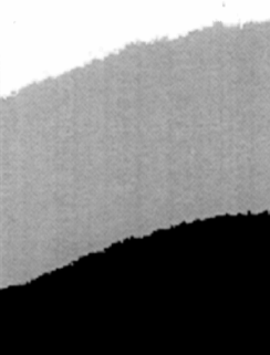
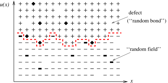
Figure 1: An Ising magnet at low temperatures forms a domain wall described by a function $u(x)$ (right). An experiment on a thin Cobalt film (left) [6]; with kind permission of the authors.

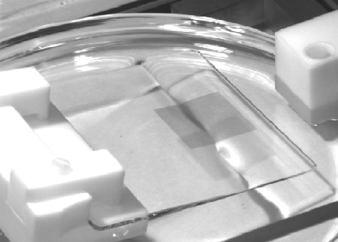
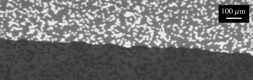
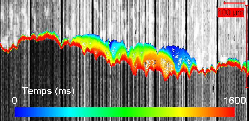
Figure 2: A contact line for the wetting of a disordered substrate by Glycerine [7]. Experimental setup (left). The disorder consists of randomly deposited islands of Chromium, appearing as bright spots (top right). Temporal evolution of the retreating contact-line (bottom right). Note the different scales parallel and perpendicular to the contact-line. Pictures courtesy of S. Moulinet, with kind permission.

Figure 3: Cartoon of an elastic lattice (e.g. vortex lattice) deformed by disorder. This is described by a vector $\vec{u}(x)$.

Before developing the theory to treat elastic systems in a disordered environment, let us give some physical realizations. The simplest one is an Ising magnet. Imposing boundary conditions with all spins up at the upper and all spins down at the lower boundary (see figure 1), at low temperatures, a domain wall separates a region with spin up from a region with spin down. In a pure system at temperature $T=0$, this domain wall is completely flat. Disorder can deform the domain wall, making it eventually rough again. Two types of disorder are common: random bond (which on a course-grained level also represents missing spins) and random field (coupling of the spins to an external random magnetic field). Figure 1 shows, how the domain wall is described by a displacement field $u(x)$. Another example is the contact line of water (or liquid Helium), wetting a rough substrate, see figure 2. (The elasticity is long range). A realization with a 2-parameter displacement field $\vec{u}(\vec{x})$ is the deformation of a vortex lattice: the position of each vortex is deformed from $\vec{x}$ to $\vec{x}+\vec{u}(\vec{x})$. A 3-dimensional example are charge density waves.

All these models have in common, that they are described by a displacement field

$$x\in\mathbb{R}^{d}\ \longrightarrow\ \vec{u}(x)\in\mathbb{R}^{N}\ .$$ (1)

For simplicity, we set $N=1$ in the following. After some initial coarse-graining, the energy ${\cal H}={\cal H}_{\mathrm{el}}+{\cal H}_{\mathrm{DO}}$ consists out of two parts: the elastic energy

$${\cal H}_{\mathrm{el}}[u]=\int{\mathrm{d}}^{d}x\,\frac{1}{2}\left(\nabla u(x)\right)^{2}$$ (2)

and the disorder

$${\cal H}_{\mathrm{DO}}[u]=\int{\mathrm{d}}^{d}x\,V(x,u(x))\ .$$ (3)

In order to proceed, we need to specify the correlations of disorder. Suppose that fluctuations $u$ in the transversal direction scale as

$$\overline{\left[u(x)-u(y)\right]^{2}}\sim|x-y|^{2\zeta}$$ (4)

with a roughness-exponent $\zeta<1$. Starting from a disorder correlator

$$\overline{V(x,u)V(x^{\prime},u^{\prime})}=f(x-x^{\prime})R(u-u^{\prime})$$ (5)

and performing one step in the RG-procedure, one has to rescale more in the $x$-direction than in the $u$-direction. This will eventually reduce $f(x-x^{\prime})$ to a $\delta$-distribution, whereas the structure of $R(u-u^{\prime})$ remains visible. We therefore choose as our starting model

$$\overline{V(x,u)V(x^{\prime},u^{\prime})}:=\delta^{d}(x-x^{\prime})R(u-u^{\prime})\ .$$ (6)

There are a couple of useful observables. We already mentioned the roughness-exponent $\zeta$. The second is the renormalized (effective) disorder. It will turn out that we actually have to keep the whole disorder distribution function $R(u)$, in contrast to keeping a few moments. Other observables are higher correlation functions or the free energy.

3 Treatment of disorder

Having defined our model, we can now turn to the treatment of disorder. The problem is to average not the partition-function, but the free energy over disorder: $\overline{{\cal F}}=-k_{\mathrm{B}}T\,\overline{\ln Z}$. This can be achieved by the beautiful replica-trick. The idea is to write

$$\ln{\cal Z}=\lim_{n\to 0}\frac{1}{n}\left({\mathrm{e}}^{n\ln{\cal Z}}-1\right)=\lim_{n\to 0}\frac{1}{n}\left({\cal Z}^{n}-1\right)$$ (7)

and to interpret ${\cal Z}^{n}$ as the partition-function of an $n$ times replicated system. Averaging ${\mathrm{e}}^{-\sum_{a=1}^{n}{\cal H}_{a}}$ over disorder then leads to the replica-Hamiltonian

$${\cal H}[u]=\frac{1}{T}\sum_{a=1}^{n}\int{\mathrm{d}}^{d}x\,\frac{1}{2}\left(\nabla u_{a}(x)\right)^{2}-\frac{1}{2T^{2}}\sum_{a,b=1}^{n}\int{\mathrm{d}}^{d}x\,R(u_{a}(x)-u_{b}(x))\ .$$ (8)

Let us stress that one could equivalently pursue a dynamic (see section 16) or a supersymmetric formulation (section 17). We therefore should not, and in fact do not encounter, problems associated with the use of the replica-trick, as long as we work with a perturbative expansion in $R$.

4 Flory estimates

Four types of disorder have to be distinguished, resulting in different universality classes:

• Random-Bond disorder (RB): short-range correlated potential-potential correlations, i.e. short-range correlated $R(u)$.

• Random-Field disorder (RF): short-range correlated force-force correlator $\Delta(u):=-R^{\prime\prime}(u)$. As the name says, this disorder is relevant for Random-field systems, where the disorder potential is the sum over all magnetic fields in say the spin-up phase.

• Generic long-range correlated disorder: $R(u)\sim|u|^{-\gamma}$.

• Random-Periodic disorder (RP): Relevant when the disorder couples to a phase, as e.g. in charge-density waves. $R(u)=R(u+1)$, supposing that $u$ is periodic with period 1.

To get an idea how large the roughness $\zeta$ becomes in these situations, one compares the contributions of elastic energy and disorder, and demands that they scale in the same way. This estimate has first been used by Flory for self-avoiding polymers, and is therefore called the Flory estimate. Despite the fact that Flory estimates are conceptually crude, they often yield a rather good approximation. For RB this gives for an $N$-component field $u$: $\int_{x}(\nabla u)^{2}\sim\int_{x}\sqrt{\overline{VV}}$, or $L^{d-2}u^{2}\sim L^{d}\sqrt{L^{-d}u^{-N}}$, i.e. $u\sim L^{\zeta}$ with

$$\zeta_{\mathrm{Flory}}^{\mathrm{RB}}=\frac{4-d}{4+N}\ .$$ (9)

For RF it is $R^{\prime\prime}$ that is short-ranged, and we obtain

$$\zeta_{\mathrm{Flory}}^{\mathrm{RF}}=\frac{4-d}{2+N}\ .$$ (10)

For LR

$$\zeta_{\mathrm{Flory}}^{\mathrm{LR}}=\frac{4-d}{4+\gamma}$$ (11)

For RP, the amplitude of $u$ is fixed, and thus $\zeta_{\mathrm{RP}}=0$.

5 Dimensional reduction

There is a beautiful and rather mind-boggling theorem relating disordered systems to pure systems (i.e. without disorder), which applies to a large class of systems, e.g. random field systems and elastic manifolds in disorder. It is called dimensional reduction and reads as follows[8]:

Theorem: A $d$-dimensional disordered system at zero temperature is equivalent to all orders in perturbation theory to a pure system in $d-2$ dimensions at finite temperature. Moreover the temperature is (up to a constant) nothing but the width of the disorder distribution. A simple example is the 3-dimensional random-field Ising model at zero temperature; according to the theorem it should be equivalent to the pure 1-dimensional Ising-model at finite temperature. But it has been shown rigorously, that the former has an ordered phase, whereas we have all solved the latter and we know that there is no such phase at finite temperature. So what went wrong? Let us stress that there are no missing diagrams or any such thing, but that the problem is more fundamental: As we will see later, the proof makes assumptions, which are not satisfied. Nevertheless, the above theorem remains important since it has a devastating consequence for all perturbative calculations in the disorder: However clever a procedure we invent, as long as we do a perturbative expansion, expanding the disorder in its moments, all our efforts are futile: dimensional reduction tells us that we get a trivial and unphysical result. Before we try to understand why this is so and how to overcome it, let us give one more example. Dimensional reduction allows to calculate the roughness-exponent $\zeta$ defined in equation (4). We know (this can be inferred from power-counting) that the width $u$ of a $d$-dimensional manifold at finite temperature in the absence of disorder scales as $u\sim x^{(2-d)/2}$. Making the dimensional shift implied by dimensional reduction leads to

$$\overline{\left[u(x)-u(0)\right]^{2}}\sim x^{4-d}\equiv x^{2\zeta}\quad\mbox{i.e.}\quad\zeta=\frac{4-d}{2}\ .$$ (12)

6 The Larkin-length, and the role of temperature

To understand the failure of dimensional reduction, let us turn to an interesting argument given by Larkin [9]. He considers a piece of an elastic manifold of size $L$. If the disorder has correlation length $r$, and characteristic potential energy $\bar{f}$, this piece will typically see a potential energy of strength

$$E_{\mathrm{DO}}=\bar{f}\left(\frac{L}{r}\right)^{\!\frac{d}{2}}\ .$$ (13)

On the other hand, there is an elastic energy, which scales like

$$E_{\mathrm{el}}=c\,L^{d-2}\ .$$ (14)

These energies are balanced at the Larkin-length $L=L_{c}$ with

$$L_{c}=\left(\frac{c^{2}}{\bar{f}^{2}}r^{d}\right)^{\frac{1}{4-d}}\ .$$ (15)

More important than this value is the observation that in all physically interesting dimensions $d<4$, and at scales $L>L_{c}$, the membrane is pinned by disorder; whereas on small scales the elastic energy dominates. Since the disorder has a lot of minima which are far apart in configurational space but close in energy (metastability), the manifold can be in either of these minimas, and the ground-state is no longer unique. However exactly this is assumed in e.g. the proof of dimensional reduction; as is most easily seen in its supersymmetric formulation, see [10] and section 17.

Another important question is, what the role of temperature is. In (4), we had supposed that $u$ scales with the systems size, $u\sim L^{\zeta}$. From the first term in (8) we conclude that

$$T\sim L^{\theta}\ ,\qquad\theta=d-2+2\zeta$$ (16)

Temperature is irrelevant when $\theta>0$, which is the case for $d>2$, and when $\zeta>0$ even below. The RG fixed point we are looking for will thus always be at zero temperature.

From the second term in (8) we conclude that disorder scales as

$$R\sim L^{d-4+4\zeta}\ .$$ (17)

This is another way to see that $d=4$ is the upper critical dimension.

7 The functional renormalization group (FRG)

Let us now discuss a way out of the dilemma: Larkin’s argument (section 6) or Eq. (17) suggests that $4$ is the upper critical dimension. So we would like to make an $\epsilon=4-d$ expansion. On the other hand, dimensional reduction tells us that the roughness is $\zeta=\frac{4-d}{2}$ (see (12)). Even though this is systematically wrong below four dimensions, it tells us correctly that at the critical dimension $d=4$, where disorder is marginally relevant, the field $u$ is dimensionless. This means that having identified any relevant or marginal perturbation (as the disorder), we find immediately another such perturbation by adding more powers of the field. We can thus not restrict ourselves to keeping solely the first moments of the disorder, but have to keep the whole disorder-distribution function $R(u)$. Thus we need a functional renormalization group treatment (FRG). Functional renormalization is an old idea going back to the seventies, and can e.g. be found in [11]. For disordered systems, it was first proposed in 1986 by D. Fisher [12]. Performing an infinitesimal renormalization, i.e. integrating over a momentum shell à la Wilson, leads to the flow $\partial_{\ell}R(u)$, with ($\epsilon=4-d$)

$$\partial_{\ell}R(u)=\left(\epsilon-4\zeta\right)R(u)+\zeta uR^{\prime}(u)+\frac{1}{2}R^{\prime\prime}(u)^{2}-R^{\prime\prime}(u)R^{\prime\prime}(0)\ .$$ (18)

The first two terms come from the rescaling of $R$ in Eq. (17) and $u$ respectively. The last two terms are the result of the 1-loop calculations, which are derived in appendix A.

More important than the form of this equation is it actual solution, sketched in figure 4.

Figure 4: Change of $-R^{\prime\prime}(u)$ under renormalization and formation of the cusp.

After some finite renormalization, the second derivative of the disorder $R^{\prime\prime}(u)$ acquires a cusp at $u=0$; the length at which this happens is the Larkin-length. How does this overcome dimensional reduction? To understand this, it is interesting to study the flow of the second and forth moment. Taking derivatives of (18) w.r.t. $u$ and setting $u$ to 0, we obtain

$$\partial_{\ell}R^{\prime\prime}(0) = \left(\epsilon-2\zeta\right)R^{\prime\prime}(0)+R^{\prime\prime\prime}(0)^{2}\ \longrightarrow\ \left(\epsilon-2\zeta\right)R^{\prime\prime}(0)$$ (19)

$$\partial_{\ell}R^{\prime\prime\prime\prime}(0) = \epsilon R^{\prime\prime\prime\prime}(0)+3R^{\prime\prime\prime\prime}(0)^{2}+4R^{\prime\prime\prime}(0)R^{\prime\prime\prime\prime\prime}(0)\ \longrightarrow\ \epsilon R^{\prime\prime\prime\prime}(0)+3R^{\prime\prime\prime\prime}(0)^{2}\ .$$ (20)

Since $R(u)$ is an even function, and moreover the microscopic disorder is smooth (after some initial averaging, if necessary), $R^{\prime\prime\prime}(0)$ and $R^{\prime\prime\prime\prime\prime}(0)$ are 0, which we have already indicated in Eqs. (19) and (20) . The above equations for $R^{\prime\prime}(0)$ and $R^{\prime\prime\prime\prime}(0)$ are in fact closed. Equation (19) tells us that the flow of $R^{\prime\prime}(0)$ is trivial and that $\zeta=\epsilon/2\equiv\frac{4-d}{2}$. This is exactly the result predicted by dimensional reduction. The appearance of the cusp can be inferred from equation (20). Its solution is

$$R^{\prime\prime\prime\prime}(0)\hskip 0.43057pt\raisebox{-4.30554pt}[0.0pt][3.44444pt]{\rule{0.43057pt}{11.84024pt}\hskip 0.86108pt}_{\ell}=\frac{c\,{\mathrm{e}}^{\epsilon\ell}}{1-3\,c\left({\mathrm{e}}^{\epsilon\ell}-1\right)/\epsilon}\ ,\qquad c:=R^{\prime\prime\prime\prime}(0)\hskip 0.43057pt\raisebox{-4.30554pt}[0.0pt][3.44444pt]{\rule{0.43057pt}{11.84024pt}\hskip 0.86108pt}_{\ell=0}$$ (21)

Thus after a finite renormalization $R^{\prime\prime\prime\prime}(0)$ becomes infinite: The cusp appears. By analyzing the solution of the flow-equation (18), one also finds that beyond the Larkin-length $R^{\prime\prime}(0)$ is no longer given by (19) with $R^{\prime\prime\prime}(0)^{2}=0$. The correct interpretation of (19), which remains valid after the cusp-formation, is (for details see below)

$$\partial_{\ell}R^{\prime\prime}(0)=\left(\epsilon-2\zeta\right)R^{\prime\prime}(0)+R^{\prime\prime\prime}(0^{+})^{2}\ .$$ (22)

Renormalization of the whole function thus overcomes dimensional reduction. The appearance of the cusp also explains why dimensional reduction breaks down. The simplest way to see this is by redoing the proof for elastic manifolds in disorder, which in the absence of disorder is a simple Gaussian theory. Terms contributing to the 2-point function involve $R^{\prime\prime}(0)$, $TR^{\prime\prime\prime\prime}(0)$ and higher derivatives of $R(u)$ at $u=0$, which all come with higher powers of $T$. To obtain the limit of $T\to 0$, one sets $T=0$, and only $R^{\prime\prime}(0)$ remains. This is the dimensional reduction result. However we just saw that $R^{\prime\prime\prime\prime}(0)$ becomes infinite. Thus $R^{\prime\prime\prime\prime}(0)T$ may also contribute, and the proof fails.

8 Measuring the cusp

Until now the function $R(u)$, a quantity central to the FRG, was loosely described as an effective disorder correlator, which evolves under coarse-graining towards a non-analytic shape. It turns out that it can be given a precise definition as an observable [13]. Hence it can directly be computed in the numerics, as we will discuss below, and in principle, be measured in experiments. The cusp therefore is not a theoretical artefact, but a real property of the system, related to singularities or shocks, which arise in the landscape of pinning forces. Moreover, these singularities are unavoidable for a glass with multiple metastable states.

Consider our interface in a random potential, and add an external quadratic potential well, centered around $w$:

$${\cal H}_{\mathrm{tot}}^{w}[u]=\frac{m^{2}}{2}(u(x)-w)^{2}+{\cal H}_{\mathrm{el}}[u]+{\cal H}_{\mathrm{DO}}[u]\ .$$ (23)

In each sample (i.e. disorder configuration), and given $w$, one finds the minimum energy configuration. This ground state energy is

$$\hat{V}(w):=\min_{u(x)}{\cal H}_{\mathrm{tot}}^{w}[u]\ .$$ (24)

It varies with $w$ as well as from sample to sample. Its second cumulant

$$\overline{\hat{V}(w)\hat{V}(w^{\prime})}^{c}=L^{d}R(w-w^{\prime})$$ (25)

defines a function $R(w)$ which is proven [13] to be the same function computed in the field theory, defined from the zero-momentum action [14].

Physically, the role of the well is to forbid the interface to wander off to infinity. The limit of small $m$ is then taken to reach the universal limit. The factor of volume $L^{d}$ is necessary, since the width $\overline{u^{2}}$ of the interface in the well cannot grow much more than $m^{-\zeta}$. This means that the interface is made of roughly $L/L_{m}$ pieces of internal size $L_{m}\approx m$ pinned independently: (25) hence expresses the central limit theorem and $R(w)$ measures the second cumulant of the disorder seen by any one of the independent pieces.

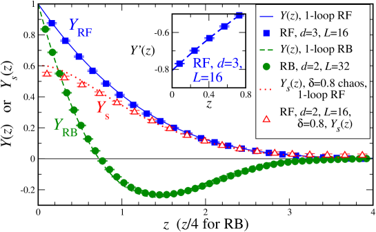
Figure 5: Filled symbols show numerical results for $Y(z)$, a normalized form of the interface displacement correlator $-R^{\prime\prime}(u)$ [Eq. (26)], for $D=2+1$ random field (RF) and $D=3+1$ random bond (RB) disorders. These suggest a linear cusp. The inset plots the numerical derivative $Y^{\prime}(z)$, with intercept $Y^{\prime}(0)\approx-0.807$ from a quadratic fit (dashed line). Open symbols plot the cross-correlator ratio $Y_{s}(z)=\Delta_{12}(z)/\Delta_{11}(0)$ between two related copies of RF disorder. It does not exhibit a cusp. The points are for confining wells with width given by $M^{2}=0.02$. Comparisons to 1-loop FRG predictions (curves) are made with no adjustable parameters. Reprinted from [15].

The nice thing about (25) is that it can be measured. One varies $w$ and computes (numerically) the new ground-state energy; finallying averaging over many realizations. This has been performed recently in [15] using a powerful exact-minimization algorithm, which finds the ground state in a time polynomial in the system size. In fact, what was measured there are the fluctuations of the center of mass of the interface $u(w)=L^{-d}\int{\mathrm{d}}^{d}x\,u_{0}(x;w)$:

$$\overline{[w-u(w)][w^{\prime}-u(w^{\prime})]}^{c}=m^{-4}L^{-d}\Delta(w-w^{\prime})$$ (26)

$w-u_{w}$

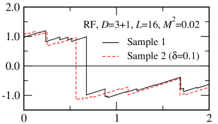
  $w$

Figure 6: Discontinuous positions, “shocks”, in $w-u_{w}$ as a function of $w$. Reprinted from [15].

which measures directly the correlator of the pinning force $\Delta(u)=-R^{\prime\prime}(u)$. To see why it is the total force, write the equilibrium condition for the center of mass $m^{2}[w-u(w)]+L^{-d}\int{\mathrm{d}}^{d}x\,F(x,u)=0$ (the elastic term vanishes if we use periodic b.c.). The result is represented in figure 5. It is most convenient to plot the function $Y=\Delta(u)/\Delta(0)$ and normalize the $u$-axis to eliminate all non-universal scales. The plot in figure 5 is free of any parameter. It has several remarkable features. First, it clearly shows that a linear cusp exists in any dimension. Next it is very close to the 1-loop prediction. Even more remarkably, as detailed in [15], the statistics is good enough to reliably compare the deviations to the 2-loop predictions obtained in section 11.

What is the physics of the cusp in $\Delta(u)$? One easily sees in a zero-dimensional model, i.e. a particle on a line, $d=0$, that as $w$ increases, the position of the minimum $u(w)$ increases smoothly, except at some discrete set of positions $w=w_{s}$, where the system switches abruptly between two distant minima. Formally, one can show that the landscape of the force $-\hat{V}^{\prime}(w)$ evolves, as the mass is lowered, according to a Burgers equation, known to develop finite-time singularities called “shocks”. For details on this mapping see [16, 13]. For an interface these shocks also exist, as can be seen on figure 6. Note that when we vary the position $w$ of the center of the well, it is not a real motion. It just means to find the new ground state for each $w$. Literally “moving” $w$ is another very interesting possibility, and will be discussed in section 16 devoted to depinning [17, 18].

9 Rounding the cusp

As we have seen, a cusp non-analyticity necessary arises at zero temperature, due to the switch-over between many metastable states. Interestingly, this cusp can be rounded by several effects: By non-zero temperature $T>0$, chaos, or a non-zero driving velocity (in the dynamics discussed below). It is easy to include the effect of temperature in the FRG equation to one loop [19]:

$$\partial_{\ell}R(u)=\left(\epsilon-4\zeta\right)R(u)+\zeta uR^{\prime}(u)+\frac{1}{2}R^{\prime\prime}(u)^{2}-R^{\prime\prime}(u)R^{\prime\prime}(0)+\tilde{T}_{\ell}R^{\prime\prime}(u)\ .$$ (27)

$\tilde{T}_{\ell}=T{\mathrm{e}}^{-\theta\ell}$ is the dimensionless temperature. It finally flows to zero, since temperature is an irrelevant variable as discussed above. Although irrelevant, it has some profound effect. Clearly the temperature in (27) acts as a diffusive term smoothening the cusp. In fact, at non-zero temperature there never is a cusp, and $R(u)$ remains analytic. The convergence to the fixed point is non-uniform. For $u$ fixed, $R(u)$ converges to the zero-temperature fixed point, except near $u=0$, or more precisely in a boundary layer of size $u\sim\tilde{T}_{\ell}$, which shrinks to zero in the large-scale limit. Non-trivial consequences are: The curvature blows up as $R^{\prime\prime\prime\prime}(0)\sim{\mathrm{e}}^{\theta\ell}/T\sim L^{\theta}/T$. One can show that this is related to the existence of thermal excitations (“droplets”) in the statics [20] and of “barriers” in the dynamics, which grow as $L^{\theta}$ [21].

Another case where rounding occurs is for “disorder chaos”. Disorder chaos is the possibility of a system to have a completely different ground state at large scales, upon a very slight change in the microscopic disorder (for instance changing slightly the magnetic field in a superconductor). Not all types of disorder exhibit chaos. Its presence in spin glasses is still debated. Recently it was investigated for elastic manifolds, using FRG [22]. One studies a model with two copies, $i=1,2$, each seeing slightly different disorder energies $V_{i}(x,u(x))$ in Eq. (3). The latter are mutually correlated gaussian random potentials with a correlation matrix

$$\overline{V_{i}(x,u)V_{j}(x^{\prime},u^{\prime})}=\delta^{d}(x-x^{\prime})R_{ij}(u-u^{\prime})\ .$$ (28)

At zero temperature, the FRG equations for $R_{11}(u)=R_{22}(u)$ are the same as in (18). The one for the cross-correlator $R_{12}(u)$ satisfies the same equation as (27) above, with $\tilde{T}_{\ell}$ is replaced by $\hat{T}:=R^{\prime\prime}_{12}(0)-R^{\prime\prime}_{11}(0)$. It is some kind of fictitious temperature, whose flow must be determined self-consistently from the two FRG equations. As in the case of a real temperature, it results in a rounding of the cusp. The physics of that is apparent from figure 6, which shows the set of shocks in two correlated samples. Since they are slightly and randomly displaced from each other, the cusp is rounded.

Chaos is obtained when $\hat{T}$ grows with scale, and occurs on scales larger than the so-called overlap length. The mutual correlations $C_{ij}(x-x^{\prime})=\overline{\left<[u^{i}(x)-u^{i}(x^{\prime})][u^{j}(x)-u^{j}(x^{\prime})]\right>}$ behave as $C_{ij}(x)=x^{2\zeta}f(\delta x^{\alpha})$, where $\delta$ quantifies the difference between the two disorders at the microscopic level. $C_{ij}(x)$ decays at large distance as $C_{ij}(x)\sim x^{2\zeta-\mu}$ [22].

10 Beyond 1 loop

Functional renormalization has successfully been applied to a bunch of problems at 1-loop order. From a field theory, we however demand more. Namely that it

$\bullet$ allows for systematic corrections beyond 1-loop order

$\bullet$ be renormalizable

$\bullet$ and thus allows to make universal predictions.

However, this has been a puzzle since 1986, and it has even been suggested that the theory is not renormalizable due to the appearance of terms of order $\epsilon^{\frac{3}{2}}$ [23]. Why is the next order so complicated? The reason is that it involves terms proportional to $R^{\prime\prime\prime}(0)$. A look at figure 3 explains the puzzle. Shall we use the symmetry of $R(u)$ to conclude that $R^{\prime\prime\prime}(0)$ is 0? Or shall we take the left-hand or right-hand derivatives, related by

$$R^{\prime\prime\prime}(0^{+}):=\lim_{{u>0}\atop{u\to 0}}R^{\prime\prime\prime}(u)=-\lim_{{u<0}\atop{u\to 0}}R^{\prime\prime\prime}(u)=:-R^{\prime\prime\prime}(0^{-}).$$ (29)

In the following, we will present our solution of this puzzle, obtained at 2-loop order, at large $N$, and in the driven dynamics.

11 Results at 2-loop order

For the flow-equation at 2-loop order, the result is [14, 24, 25, 26, 27]

$$\partial_{\ell}R(u) = \left(\epsilon-4\zeta\right)R(u)+\zeta uR^{\prime}(u)+\frac{1}{2}R^{\prime\prime}(u)^{2}-R^{\prime\prime}(u)R^{\prime\prime}(0)$$ (30)

$$+\frac{1}{2}\left(R^{\prime\prime}(u)-R^{\prime\prime}(0)\right)R^{\prime\prime\prime}(u)^{2}-\frac{1}{2}R^{\prime\prime\prime}(0^{+})^{2}R^{\prime\prime}(u)\ .$$

The first line is the result at 1-loop order, already given in (18). The second line is new. The most interesting term is the last one, which involves $R^{\prime\prime\prime}(0^{+})^{2}$ and which we therefore call anomalous. The hard task is to fix the prefactor $(-\frac{1}{2})$. We have found five different prescriptions to calculate it: The sloop-algorithm, recursive construction, reparametrization invariance, renormalizability, and potentiality [24, 14]. For lack of space, we restrain our discussion to the last two ones. At 2-loop order the following diagram appears

$$\parbox{62.53679pt}{\hskip 3.44444pt\includegraphics[scale={0.35}]{./figures/subdiv}\hskip 3.44444pt}\ \longrightarrow\ \frac{1}{2}\left(R^{\prime\prime}(u)-R^{\prime\prime}(0)\right)R^{\prime\prime\prime}(u)^{2}-\frac{1}{2}R^{\prime\prime}(u)R^{\prime\prime\prime}(0^{+})^{2}$$ (31)

leading to the anomalous term. The integral (not written here) contains a sub-divergence, which is indicated by the box. Renormalizability demands that its leading divergence (which is of order $1/\epsilon^{2}$) be canceled by a 1-loop counter-term. The latter is unique thus fixing the prefactor of the anomalous term. (The idea is to take the 1-loop correction $\delta R$ in Eq. (81) and replace one of the $R^{\prime\prime}$ in it by $\delta R^{\prime\prime}$ itself, which the reader can check to leading to the terms given in (31) plus terms which only involve even derivatives.)

Another very physical demand is that the problem remain potential, i.e. that forces still derive from a potential. The force-force correlation function being $-R^{\prime\prime}(u)$, this means that the flow of $R^{\prime}(0)$ has to be strictly 0. (The simplest way to see this is to study a periodic potential.) From (11) one can check that this does not remain true if one changes the prefactor of the last term in (11); thus fixing it.

Let us give some results for cases of physical interest. First of all, in the case of a periodic potential, which is relevant for charge-density waves, the fixed-point function can be calculated analytically as (we choose period 1, the following is for $u\in\left[0,1\right]$)

$$R^{*}(u)=-\left(\frac{\epsilon}{72}+\frac{\epsilon^{2}}{108}+O(\epsilon^{3})\right)u^{2}(1-u)^{2}+\mbox{const.}$$ (32)

This leads to a universal amplitude. In the case of random-field disorder (short-ranged force-force correlation function) $\zeta=\frac{\epsilon}{3}$, equivalent to the Flory estimate (10). For random-bond disorder (short-ranged potential-potential correlation function) we have to solve (30) numerically, with the result

$$\zeta=0.20829804\epsilon+0.006858\epsilon^{2}+O(\epsilon^{3})\ .$$ (33)

This compares well with numerical simulations, see figure 7. It is also surprisingly close, but distinctly different, from the Flory estimate (9), $\zeta=\epsilon/5$.

$\zeta$ one loop two loop estimate simulation and exact $d=3$ 0.208 0.215 $0.215\pm 0.01$ $0.22\pm 0.01$ [28] $d=2$ 0.417 0.444 $0.42\pm 0.02$ $0.41\pm 0.01$ [28] $d=1$ 0.625 0.687 $0.67\pm 0.02$ $2/3$

Figure 7: Results for $\zeta$ in the random bond case.

12 Finite $N$

Up to now, we have studied the functional RG for one component $N=1$. The general case of finite $N$ is more difficult to handle, since derivatives of the renormalized disorder now depend on the direction, in which this derivative is taken. Define amplitude $u:=|\vec{u}|$ and direction $\hat{u}:=\vec{u}/|\vec{u}|$ of the field. Then deriving the latter variable leads to terms proportional to $1/u$, which are diverging in the limit of $u\to 0$. This poses additional problems in the calculation, and it is a priori not clear that the theory at $N\neq 1$ exists, supposed this is the case for $N=1$. At 1-loop order everything is well-defined [23]. We have found a consistent RG-equation at 2-loop order [29]:

Figure 8: Results for the roughness $\zeta$ at 1- and 2-loop order, as a function of the number of components $N$.

$$\partial_{\ell}R(u) = (\epsilon-4\zeta)R(u)+\zeta uR^{\prime}(u)+\frac{1}{2}R^{\prime\prime}(u)^{2}-R^{\prime\prime}(0)R^{\prime\prime}(u)+\frac{N-1}{2}\frac{R^{\prime}(u)}{u}\left(\frac{R^{\prime}(u)}{u}-2R^{\prime\prime}(0)\right)$$ (34)

$$+\frac{1}{2}\left(R^{\prime\prime}(u)-R^{\prime\prime}(0)\right)\,{R^{\prime\prime\prime}(u)}^{2}+\frac{N{-}1}{2}\frac{{\left(R^{\prime}(u){-}uR^{\prime\prime}(u)\right)}^{2}\,(2R^{\prime}(u){+}u(R^{\prime\prime}(u){-}3R^{\prime\prime}(0)))}{u^{5}}$$

$$-R^{\prime\prime\prime}(0^{+})^{2}\left[\frac{N+3}{8}R^{\prime\prime}(u)+\frac{N-1}{4}\frac{R^{\prime}(r)}{u}\right]\ .$$

The first line is the 1-loop equation, given in [23]. The second and third line represent the 2-loop equation, with the new anomalous terms proportional to $R^{\prime\prime\prime}(0^{+})^{2}$ (third line).

The fixed-point equation (34) can be integrated numerically, order by order in $\epsilon$. The result, specialized to directed polymers, i.e. $\epsilon=3$ is plotted on figure 8. We see that the 2-loop corrections are rather big at large $N$, so some doubt on the applicability of the latter down to $\epsilon=3$ is advised. However both 1- and 2-loop results reproduce well the two known points on the curve: $\zeta=2/3$ for $N=1$ and $\zeta=0$ for $N=\infty$. The latter result will be given in section 13. Via the equivalence [30] of the directed-polymer problem in $N$ dimensions treated here and the KPZ-equation of non-linear surface growth in $N$ dimensions, which relate the roughness exponent $\zeta$ of the directed polymer to the dynamic exponent $z_{\mathrm{KPZ}}$ in the KPZ-equation via $\zeta=\frac{1}{z_{{\mathrm{KPZ}}}}$, we know that $\zeta(N=1)=2/3$.

The line $\zeta=1/2$ given on figure 8 plays a special role: In the presence of thermal fluctuations, we expect the roughness-exponent of the directed polymer to be bounded by $\zeta\geq 1/2$. In the KPZ-equation, this corresponds to a dynamic exponent $z_{\mathrm{KPZ}}=2$, which via the exact scaling relation $z_{\mathrm{KPZ}}+\zeta_{\mathrm{KPZ}}=2$ is an upper bound in the strong-coupling phase. The above data thus strongly suggest that there exists an upper critical dimension in the KPZ-problem, with $d_{\mathrm{uc}}\approx 2.4$. Even though the latter value might be an underestimation, it is hard to imagine what can go wrong qualitatively with this scenario. The strongest objections will probably arise from numerical simulations, such as [31]. However the latter use a discrete RSOS model, and the exponents are measured for interfaces, which in large dimensions have the thickness of the discretization size, suggesting that the data are far from the asymptotic regime. We thus strongly encourage better numerical simulations on a continuous model, in order to settle this issue.

13 Large $N$

In the last sections, we have discussed renormalization in a loop expansion, i.e. expansion in $\epsilon$. In order to independently check consistency, it is good to have a non-perturbative approach. This is achieved by the large-$N$ limit, which can be solved analytically and to which we turn now. We start from

$${\cal H}[\vec{u},\vec{j}] = \frac{1}{2T}\sum_{a=1}^{n}\int_{x}\vec{u}_{a}(x)\left(-\nabla^{2}{+}m^{2}\right)\vec{u}_{a}(x)-\sum_{a=1}^{n}\int_{x}\vec{j}_{a}(x)\vec{u}_{a}(x)$$ (35)

$$-\frac{1}{2T^{2}}\sum_{a,b=1}^{n}\int_{x}B\left((\vec{u}_{a}(x)-\vec{u}_{b}(x))^{2}\right)\ .$$

where in contrast to (8), we use an $N$-component field $\vec{u}$. For $N=1$, we identify $B(u^{2})=R(u)$. We also have added a mass $m$ to regularize the theory in the infra-red and a source $\vec{j}$ to calculate the effective action $\Gamma(\vec{u})$ via a Legendre transform. For large $N$ the saddle-point equation reads [32]

$$\tilde{B}^{\prime}(u_{ab}^{2})=B^{\prime}\left(u_{ab}^{2}+2TI_{1}+4I_{2}[\tilde{B}^{\prime}(u_{ab}^{2})-\tilde{B}^{\prime}(0)]\right)\ .$$ (36)

This equation gives the derivative of the effective (renormalized) disorder $\tilde{B}$ as a function of the (constant) background field $u_{ab}^{2}=(u_{a}-u_{b})^{2}$ in terms of: the derivative of the microscopic (bare) disorder $B$, the temperature $T$ and the integrals $I_{n}:=\int_{k}\frac{1}{\left(k^{2}+m^{2}\right)^{n}}$.

The saddle-point equation can again be turned into a closed functional renormalization group equation for $\tilde{B}$ by taking the derivative w.r.t. $m$:

$$\partial_{\ell}\tilde{B}(x)\equiv-\frac{m\partial}{\partial m}\tilde{B}(x)=\left(\epsilon-4\zeta\right)\!\tilde{B}(x)+2\zeta x\tilde{B}^{\prime}(x)+\frac{1}{2}\tilde{B}^{\prime}(x)^{2}-\tilde{B}^{\prime}(x)\tilde{B}^{\prime}(0)+\frac{\epsilon\,T\tilde{B}^{\prime}(x)}{\epsilon+\tilde{B}^{\prime\prime}(0)}\,\,\,$$ (37)

This is a complicated nonlinear partial differential equation. It is therefore surprising, that one can find an analytic solution. (The trick is to write down the flow-equation for the inverse function of $\tilde{B}^{\prime}(x)$, which is linear.) Let us only give the results of this analytic solution: First of all, for long-range correlated disorder of the form $\tilde{B}^{\prime}(x)\sim x^{-\gamma}$, the exponent $\zeta$ can be calculated analytically as $\zeta=\frac{\epsilon}{2(1+\gamma)}\ .$ It agrees with the replica-treatment in [33], the 1-loop treatment in [23], and the Flory estimate (11). For short-range correlated disorder, $\zeta=0$. Second, it demonstrates that before the Larkin-length, $\tilde{B}(x)$ is analytic and thus dimensional reduction holds. Beyond the Larkin length, $\tilde{B}^{\prime\prime}(0)=\infty$, a cusp appears and dimensional reduction is incorrect. This shows again that the cusp is not an artifact of the perturbative expansion, but an important property even of the exact solution of the problem (here in the limit of large $N$).

14 Relation to Replica Symmetry Breaking (RSB)

There is another treatment of the limit of large $N$ given by Mézard and Parisi [33]. They start from (35) but without a source-term $j$. In the limit of large $N$, a Gaussian variational ansatz of the form

$${\cal H}_{\mathrm{g}}[\vec{u}] = \frac{1}{2T}\sum_{a=1}^{n}\int_{x}\vec{u}_{a}(x)\left(-\nabla^{2}{+}m^{2}\right)\vec{u}_{a}(x)-\frac{1}{2T^{2}}\sum_{a,b=1}^{n}\sigma_{ab}\,\vec{u}_{a}(x)\vec{u}_{b}(x)$$ (38)

becomes exact. The art is to make an appropriate ansatz for $\sigma_{ab}$. The simplest possibility, $\sigma_{ab}=\sigma$ for all $a\neq b$ reproduces the dimensional reduction result, which breaks down at the Larkin length. Beyond that scale, a replica symmetry broken (RSB) ansatz for $\sigma_{ab}$ is suggestive. To this aim, one can break $\sigma_{ab}$ into four blocks of equal size, choose one (variationally optimized) value for the both outer diagonal blocks, and then iterate the procedure on the diagonal blocks, resulting in

$$\sigma_{ab}=\left(\,\parbox{127.5pt}{\includegraphics[width=127.5pt]{./figures/RSBmatrice}}\,\right)\ .$$ (39)

Figure 9: The function $\left[\sigma\right](u)+m^{2}$ as given in [33].

One finds that the more often one iterates, the better the result becomes. In fact, one has to repeat this procedure infinite many times. This seems like a hopeless endeavor, but Parisi has shown that the infinitely often replica symmetry broken matrix can be parameterized by a function $[\sigma](z)$ with $z\in\left[0,1\right]$. In the SK-model, $z$ has the interpretation of an overlap between replicas. While there is no such simple interpretation for the model (38), we retain that $z=0$ describes distant states, whereas $z=1$ describes nearby states. The solution of the large-$N$ saddle-point equations leads to the curve depicted in figure 6. Knowing it, the 2-point function is given by

$$\left<u_{k}u_{-k}\right>=\frac{1}{k^{2}+m^{2}}\left(1+\int_{0}^{1}\frac{{\mathrm{d}}z}{z^{2}}\frac{\left[\sigma\right](z)}{k^{2}+\left[\sigma\right](z)+m^{2}}\right)\ .$$ (40)

The important question is: What is the relation between the two approaches, which both declare to calculate the same 2-point function? Comparing the analytical solutions, we find that the 2-point function given by FRG is the same as that of RSB, if in the latter expression we only take into account the contribution from the most distant states, i.e. those for $z$ between 0 and $z_{m}$ (see figure 9). To understand why this is so, we have to remember that the two calculations were done under quite different assumptions: In contrast to the RSB-calculation, the FRG-approach calculated the partition function in presence of an external field $j$, which was then used to give via a Legendre transformation the effective action. Even if the field $j$ is finally tuned to 0, the system will remember its preparation, as is the case for a magnet: Preparing the system in presence of a magnetic field will result in a magnetization which aligns with this field. The magnetization will remain, even if finally the field is turned off. The same phenomena happens here: By explicitly breaking the replica-symmetry through an applied field, all replicas will settle in distant states, and the close states from the Parisi-function $\left[\sigma\right](z)+m^{2}$ (which describes spontaneous RSB) will not contribute. However, we found that the full RSB-result can be reconstructed by remarking that the part of the curve between $z_{m}$ and $z_{c}$ is independent of the infrared cutoff $m$, and then integrating over $m$ [32] ($m_{c}$ is the mass corresponding to $z_{c}$):

$$\left<u_{k}u_{-k}\right>\Big{|}^{\mathrm{RSB}}_{k=0}=\frac{\tilde{R}^{\prime}_{m}(0)}{m^{4}}+\int_{m}^{m_{c}}\frac{{\mathrm{d}}\tilde{R}^{\prime}_{\mu}(0)}{\mu^{4}}+\frac{1}{m_{c}^{2}}-\frac{1}{m^{2}}\ .$$ (41)

We also note that a similar effective action has been proposed in [16]. While it agrees qualitatively, it does not reproduce the correct FRG 2-point function, as it should.

15 Corrections at order $1/N$

In a graphical notation, we find [34]

$$\delta B^{(1)} = \!\!\parbox{56.03249pt}{\hskip 3.44444pt\includegraphics[scale={0.35}]{./figures/1oN1}\hskip 3.44444pt}\!\!+\!\!\!\parbox{50.25089pt}{\hskip 3.44444pt\includegraphics[scale={0.35}]{./figures/1oN2}\hskip 3.44444pt}\!\!+\!\!\parbox{53.86438pt}{\hskip 3.44444pt\includegraphics[scale={0.35}]{./figures/1oN3}\hskip 3.44444pt}\!\!+\!\!\!\parbox{37.24228pt}{\hskip 3.44444pt\includegraphics[scale={0.35}]{./figures/1oN4}\hskip 3.44444pt}\!\!+\!\!\parbox{28.56989pt}{\hskip 3.44444pt\includegraphics[scale={0.35}]{./figures/1oN5}\hskip 3.44444pt}\!\!$$ (42)

$$+T\Big{(}\!\!\parbox{37.24228pt}{\hskip 3.44444pt\includegraphics[scale={0.35}]{./figures/1oNT1a}\hskip 3.44444pt}\!\!+\!\!\parbox{28.56989pt}{\hskip 3.44444pt\includegraphics[scale={0.35}]{./figures/1oNT1b}\hskip 3.44444pt}\!\!+\!\!\parbox{50.97359pt}{\hskip 3.44444pt\includegraphics[scale={0.35}]{./figures/1oNT1cN}\hskip 3.44444pt}\!\!+\!\!\parbox{52.41899pt}{\hskip 3.44444pt\includegraphics[scale={0.35}]{./figures/1oNT1dN}\hskip 3.44444pt}\!\!+\!\!\parbox{34.35149pt}{\hskip 3.44444pt\includegraphics[scale={0.35}]{./figures/1oNT1b0}\hskip 3.44444pt}\!\!+\!\!\parbox{53.86438pt}{\hskip 3.44444pt\includegraphics[scale={0.35}]{./figures/1oNT1dN0}\hskip 3.44444pt}\!\!\Big{)}$$

$$+T^{2}\Big{(}\!\!\parbox{28.56989pt}{\hskip 3.44444pt\includegraphics[scale={0.35}]{./figures/1oNT2a}\hskip 3.44444pt}\!\!+\!\!\parbox{28.56989pt}{\hskip 3.44444pt\includegraphics[scale={0.35}]{./figures/1oNT2bN}\hskip 3.44444pt}\!\!+\!\!\parbox{53.86438pt}{\hskip 3.44444pt\includegraphics[scale={0.35}]{./figures/1oNT2cN}\hskip 3.44444pt}+{\cal A}^{T^{2}}\Big{)}$$

$$= B^{\prime\prime}(\chi_{ab})\left(1-4A_{d}I_{2}(p)B^{\prime\prime}(\chi_{ab})\right)^{-1}\ ,\quad\parbox{10.50238pt}{\hskip 3.44444pt\includegraphics[scale={0.35}]{./figures/B}\hskip 3.44444pt}=B(\chi_{ab})\ ,$$ (43)

where the explicit expressions are given in [34].

By varying the IR-regulator, one can derive a $\beta$-function at order $1/N$, see [34]. At $T=0$, it is UV-convergent, and should allow to find a fixed point. We have been able to do this at order $\epsilon$, showing consistency with the 1-loop result, see section 12. Other dimensions are more complicated.

A $\beta$-function can also be defined at finite $T$. However since temperature is an irrelevant variable, it makes the theory non-renormalizable, i.e. in order to define it, one must keep an explicit infrared cutoff. These problems have not yet been settled.

16 Depinning transition

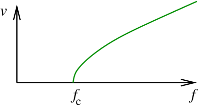
Figure 10: Velocity of a pinned interface as a function of the applied force. Zero force: equilibrium. $f=f_{c}$: depinning.

Another important class of phenomena for elastic manifolds in disorder is the so-called “depinning transition”: Applying a constant force to the elastic manifold, e.g. a constant magnetic field to the ferromagnet mentioned in the introduction, the latter will only move, if a certain critical threshold force $f_{c}$ is surpassed, see figure 10. (This is fortunate, since otherwise the magnetic domain walls in the hard-disc drive onto which this article is stored would move with the effect of deleting all information, depriving the reader from his reading.) At $f=f_{c}$, the so-called depinning transition, the manifold has a distinctly different roughness exponent $\zeta$ (see Eq. (4)) from the equilibrium ($f=0$). For $f>f_{c}$, the manifold moves, and close to the transition, new observables and corresponding exponents appear:

• the dynamic exponent $z$ relating correlation functions in spatial and temporal direction

  $$t\sim x^{\,z}$$

• a correlation length $\xi$ set by the distance to $f_{c}$

  $$\xi\sim|f-f_{c}|^{-\nu}$$

• furthermore, the new exponents are not all independent, but satisfy the following exponent relations [35]

  $$\beta=\nu(z-\zeta)\qquad\qquad\nu=\frac{1}{2-\zeta}$$ (44)

The equation describing the movement of the interface is

$$\partial_{t}u(x,t)=(\nabla^{2}+m^{2})u(x,t)+F(x,u(x,t))\ ,\qquad F(x,u)=-\partial_{u}V(x,u)$$ (45)

This model has been treated at 1-loop order by Natterman et al. [35] and by Narayan and Fisher [36]. The 1-loop flow-equations are identical to those of the statics. This is surprising, since physically, the phenomena at equilibrium and at depinning are quite different. There is even the claim by [36], that the roughness exponent in the random field universality class is exactly $\zeta=\epsilon/3$, as it is in the equilibrium random field class. After a long debate among numerical physicists, the issue is today resolved: The roughness is significantly larger, and reads e.g. for the driven polymer $\zeta=1.25$, instead of $\zeta=1$ as predicted in [36]. Clearly, a 2-loop analysis [37] is necessary, to resolve these issues. Such a treatment starts from the dynamic action

$${\cal S}=\int_{x,t}\tilde{u}(x,t)(\partial_{t}-\nabla^{2}+m^{2})u(x,t)+\int_{x,t,t^{\prime}}\tilde{u}(x,t)\Delta(u(x,t)-u(x,t^{\prime}))\tilde{u}(x,t^{\prime})\ ,$$ (46)

where the “response field” $\tilde{u}(x,t)$ enforces the equation of motion (45) and

$$\overline{F(x,u)F(x^{\prime},u^{\prime})}=\Delta(u-u^{\prime})\delta^{d}(x-x^{\prime})\equiv-R^{\prime\prime}(u-u^{\prime})\delta^{d}(x-x^{\prime})$$ (47)

is the force-force correlator, leading to the second term in (46). As in the statics, one encounters terms proportional to $\Delta^{\prime}(0^{+})\equiv-R^{\prime\prime\prime}(0^{+})$. Here the sign-problem can uniquely be solved by observing that the membrane only jumps ahead,

$$t>t^{\prime}\qquad\Rightarrow\qquad u(x,t)\geq u(x,t^{\prime})\ .$$ (48)

Practically this means that when evaluating diagrams containing $\Delta(u(x,t)-u(x,t^{\prime}))$, one splits them into two pieces, one with $t<t^{\prime}$ and one with $t>t^{\prime}$. Both pieces are well defined, even in the limit of $t\to t^{\prime}$. As the only tread-off of this method, diagrams can become complicated and difficult to evaluate; however they are always well-defined.

	$d$	$\epsilon$	$\epsilon^{2}$	estimate	simulation
	$3$	0.33	0.38	0.38$\pm$0.02	0.34$\pm$0.01
$\zeta$	$2$	0.67	0.86	0.82$\pm$0.1	0.75$\pm$0.02
	$1$	1.00	1.43	1.2$\pm$0.2	1.25$\pm$0.01
	$3$	0.89	0.85	0.84$\pm$0.01	0.84$\pm$0.02
$\beta$	$2$	0.78	0.62	0.53$\pm$0.15	0.64$\pm$0.02
	$1$	0.67	0.31	0.2$\pm$0.2	0.25 …0.4
	$3$	0.58	0.61	0.62$\pm$0.01
$\nu$	$2$	0.67	0.77	0.85$\pm$0.1	0.77$\pm$0.04
	$1$	0.75	0.98	1.25$\pm$0.3	1$\pm$0.05

	$\epsilon$	$\epsilon^{2}$	estimate	simulation
$\zeta$	0.33	0.47	0.47$\pm$0.1	0.39$\pm$0.002
$\beta$	0.78	0.59	0.6$\pm$0.2	0.68$\pm$0.06
$z$	0.78	0.66	0.7$\pm$0.1	0.74$\pm$0.03
$\nu$	1.33	1.58	2$\pm$0.4	1.52$\pm$0.02

Figure 11: The critical exponents at the depinning transition, for short range elasticity (left) and for long range elasticity (right).

Physically, this means that we approach the depinning transition from above. This is reflected in (48) by the fact that $u(x,t)$ may remain constant; and indeed correlation-functions at the depinning transition are completely independent of time[37]. On the other hand a theory for the approach of the depinning transition from below ($f<f_{c}$) has been elusive so far.

At the depinning transition, the 2-loop functional RG reads [24, 37]

$$\partial_{\ell}R(u)\! = \!(\epsilon-4\zeta)R(u)+\zeta uR^{\prime}(u)+\frac{1}{2}R^{\prime\prime}(u)^{2}{-}R^{\prime\prime}(u)R^{\prime\prime}(0)$$ (49)

$$+\frac{1}{2}\,\left[R^{\prime\prime}(u)-R^{\prime\prime}(0)\right]R^{\prime\prime\prime}(u)^{2}~{}{\mbox{\bf+}}~{}\frac{1}{2}\,R^{\prime\prime\prime}(0^{+})^{2}R^{\prime\prime}(u)$$

First of all, note that it is a priori not clear that the functional RG equation, which is a flow equation for $\Delta(u)=-R^{\prime\prime}(u)$ can be integrated to a functional RG-equation for $R(u)$. We have chosen this representation here, in order to make the difference to the statics evident: The only change is in the last sign on the second line of (49). This has important consequences for the physics: First of all, the roughness exponent $\zeta$ for the random-field universality class changes from $\zeta=\frac{\epsilon}{3}$ to

$$\zeta=\frac{\epsilon}{3}(1+0.14331\epsilon+\ldots)$$ (50)

Second, the random-bond universality class is unstable and always renormalizes to the random-field universality class, as is physically expected: Since the membrane only jumps ahead, it always experiences a new disorder configuration, and there is no way to know of whether this disorder can be derived from a potential or not. Generalizing the arguments of section 8, it has recently been confirmed numerically that both RB and RF disorder flow to the RF fixed point [17, 18], and that this fixed point is very close to the solution of (49), see figure 12.

\psfrag{random-field-disorder-num}{\small RF $m=0.071$, $L=512$}\psfrag{random-bond-disorder-num}{\small RB $m=0.071$, $L=512$}\psfrag{y}{\small$Y(z)$}\psfrag{x}{\small$z$}\includegraphics[width=256.0748pt]{./figures/Delta}

Figure 12: Universal scaling form $Y(z)$ for $\Delta(u)$ for RB and RF disorder. Reprinted from [18].

This non-potentiality is most strikingly observed in the random periodic universality class, which is the relevant one for charge density waves. The fixed point for a periodic disorder of period one reads (remember $\Delta(u)=-R^{\prime\prime}(u)$)

$$\Delta^{*}(u)=\frac{\epsilon}{36}+\frac{\epsilon^{2}}{108}-\left(\frac{\epsilon}{6}+\frac{\epsilon^{2}}{9}\right)u(1-u)$$ (51)

Integrating over a period, we find (suppressing in $F(x,u)$ the dependence on the coordinate $x$ for simplicity of notation)

$$\int_{0}^{1}{\mathrm{d}}u\,\Delta^{*}(u)\equiv\int_{0}^{1}{\mathrm{d}}u\ \overline{F(u)F(u^{\prime})}=-\frac{\epsilon^{2}}{108}\ .$$ (52)

In an equilibrium situation, this correlator would vanish, since potentiality requires $\int_{0}^{1}{\mathrm{d}}u\,F(u)\equiv 0$. Here, there are non-trivial contributions at 2-loop order (order $\epsilon^{2}$), violating this condition and rendering the problem non-potential. This same mechanism is also responsible for the violation of the conjecture $\zeta=\frac{\epsilon}{3}$, which could be proven on the assumption that the problem remains potential under renormalization. Let us stress that the breaking of potentiality under renormalization is a quite novel observation here.

The other critical exponents mentioned above can also be calculated. The dynamical exponent $z$ (for RF-disorder) reads [24, 37]

$$z=2-\frac{2}{9}\epsilon-0.04321\epsilon^{2}+\ldots$$ (53)

All other exponents are related via the relation (44). That the method works well even quantitatively can be inferred from figure 11.

17 Supersymmetry

The use of $n$ replicas in the limit $n\to 0$ to describe disordered systems is often criticized for a lack of rigor. It is argued that instead one should use a supersymmetric formulation. Such a formulation is indeed possible, both for the statics as discussed in [38], as for the dynamics, which we will discuss below. Following [10], one groups the field $u(x)$, a bosonic auxiliary field $\tilde{u}(x)$ and two Grassmanian fields $\psi(x)$ and $\bar{\psi}(x)$ into a superfield $U(x,\bar{\Theta},\Theta)$:

$$U(x,\bar{\Theta},\Theta)=u(x)+\bar{\Theta}\psi(x)+\bar{\psi}(x)\Theta+\Theta\bar{\Theta}\tilde{u}(x)\ .$$ (54)

The action of the supersymmetric theory is

$${\cal S}_{\mathrm{Susy}}=\int{\mathrm{d}}\Theta{\mathrm{d}}\bar{\Theta}\int_{x}U(x,\bar{\Theta},\Theta)(\Delta_{s})U(x,\bar{\Theta},\Theta)\ ,\qquad\Delta_{s}:=\nabla^{2}-\Delta(0)\frac{\partial}{\partial\bar{\Theta}}\frac{\partial}{\partial\Theta}$$ (55)

It is invariant under the action of the supergenerators

$$Q:=x\frac{\partial}{\partial\Theta}-\frac{2}{\Delta(0)}\bar{\Theta}\nabla\ ,\qquad\bar{Q}:=x\frac{\partial}{\partial\bar{\Theta}}+\frac{2}{\Delta(0)}\Theta\nabla\ .$$ (56)

What do the fields mean? Upon integrating over $\bar{\Theta}$ and $\Theta$ before averaging over disorder, one would obtain two terms, $\sim\int_{x}\tilde{u}(x)\frac{\delta{\cal H}}{\delta u(x)}$, i.e. the bosonic auxiliary field $\tilde{u}(x)$ enforces $\frac{\delta{H}}{\delta u(x)}=0$, and a second term, bilenear in $\bar{\psi}$ and $\psi$, $\sim\int_{x}\bar{\psi}\frac{\delta^{2}{\cal H}}{\delta u^{2}}\psi$ which ensures that the partition function is one. (55) is nothing but the dimensional reduction result (12) in super-symmetric disguise. What went wrong? Missing is the renormalization of $R(u)$ itself, which in the FRG approach leads to a flow of $\Delta(0)\equiv-R^{\prime\prime}(0)$. In order to capture this, one has to look at the supersymmetric action of at least two copies:

$${\cal S}[U_{a}]=\sum_{a}\int_{\Theta,\bar{\Theta}}\int_{x}U_{a}(x,\bar{\Theta},\Theta)(\Delta_{s})U_{a}(x,\bar{\Theta},\Theta)-\frac{1}{2}\sum_{a\neq b}\int_{x}\int_{\bar{\Theta},\Theta}\int_{\bar{\Theta}^{\prime},\Theta^{\prime}}R(U_{a}(x,\bar{\Theta},\Theta)-U_{b}(x,\bar{\Theta}^{\prime},\Theta^{\prime}))\ .$$ (57)

Formally, we have again introduced $n$ replicas, but we do not take the limit of $n\to 0$; so criticism of the latter limit can not be applied here. After some slightly cumbersome calculations one reproduces the functional RG $\beta$-function at 1-loop (18). (Higher orders are also possible and the SUSY method is actually helpful [38].) At the Larkin-length, where the functional RG produces a cusp, the flow of $\Delta(0)$ becomes non-trivial, given in (22). Then the parameter $\Delta(0)$ in the supersymmetry generators (56) is no longer a constant, and supersymmetry breaks down. This is, as was discussed in section (14), also the onset of replica-symmetry breaking in the gaussian variational ansatz, valid at large $N$.

Another way to introduce a supersymmetric formulation proceeds via the super-symmetric representation of a stochastic equation of motion [39]; a method e.g. used in [40] to study spin-glasses. The action then changes to

$${\cal S}[U]=\int_{xt}\int_{\Theta,\bar{\Theta}}U(x,\bar{\Theta},\Theta,t)(\Delta_{d})U(x,\bar{\Theta},\Theta,t)-\frac{1}{2}\int_{xtt^{\prime}}\int_{\bar{\Theta},\Theta}\int_{\bar{\Theta}^{\prime},\Theta^{\prime}}R(U(x,\bar{\Theta},\Theta,t)-U(x,\bar{\Theta}^{\prime},\Theta^{\prime},t^{\prime}))\ .$$ (58)

$$\Delta_{d}=\nabla^{2}+\bar{D}D\ ,\qquad\bar{D}=\frac{\partial}{\partial\Theta}\ ,\qquad D=\frac{\partial}{\partial\bar{\Theta}}-\Theta\frac{\partial}{\partial t}$$ (59)

and is invariant under the action of the super-generators $Q:=\frac{\partial}{\partial\bar{\Theta}}$ and $\bar{Q}:=\frac{\partial}{\partial\Theta}+\bar{\Theta}\frac{\partial}{\partial t}$, since $\left\{Q,D\right\}=\left\{Q,\bar{D}\right\}=\left\{\bar{Q},D\right\}=\left\{\bar{Q},\bar{D}\right\}=0$. Different replicas now become different times, but second cumulant still means bilocal in $\Theta$. However the procedure is not much different from a pure Langevin equation of motion, as in (45); in the latter equation Itô discretization is already sufficient to ensure that the partition function is 1. The main advantage is the possibility to change the discretization procedure from Itô over mid-point to Stratonovich without having to add additional terms. In this case, supersymmetry breaking means that the system falls out of equlibrium, i.e. the fluctuation-dissipation theorem (which is a consequence of one of the supersymmetry generators [39]) breaks down [40].

18 Random Field Magnets

Another domain of application of the Functional RG is spin models in a random field. The model usually studied is:

$${\cal H}=\int{\mathrm{d}}^{d}x\,\frac{1}{2}(\nabla\vec{S})^{2}+\vec{h}(x)\cdot\vec{S}(x)\ ,$$ (60)

where $\vec{S}(x)$ is a unit vector with $N$-components, and $\vec{S}(x)^{2}=1$. This is the so-called $O(N)$ sigma model, to which has been added a random field, which can be taken gaussian $\overline{h_{i}(x)h_{j}(x^{\prime})}=\sigma\delta_{ij}\delta^{d}(x-x^{\prime})$. In the absence of disorder the model has a ferromagnetic phase for $T<T_{\mathrm{f}}$ and a paramagnetic phase above $T_{\mathrm{f}}$. The lower critical dimension is $d=2$ for any $N\geq 2$, meaning that below $d=2$ no ordered phase exists. In $d=2$ solely a paramagnetic phase exists for $N>2$; for $N=2$, the XY model, quasi long-range order exists at low temperature, with $\overline{\vec{S}(x)\vec{S}(x^{\prime})}$ decaying as a power law of $x-x^{\prime}$.

Here we study the model directly at $T=0$. The dimensional reduction theorem in section 5, which also holds for random field magnets, would indicate that the effect of a quenched random field in dimension $d$ is similar to the one of a temperature $T\sim\sigma$ for a pure model in dimension $d-2$. Hence one would expect a transition from a ferromagnetic to a disordered phase at $\sigma_{c}$ as the disorder increases in any dimension $d>4$, and no order at all for $d<4$ and $N\geq 2$. This however is again incorrect, as can be seen using FRG.

It was noticed by Fisher [41] that an infinity of relevant operators are generated. These operators, which correspond to an infinite set of random anisotropies, are irrelevant by naive power counting near $d=6$ [42, 43]. $d=6$ is the naive upper critical dimension (corresponding to $d=4$ for the pure $O(N)$ model) as indicated by dimensional reduction; so many earlier studies concentrated on $d$ around $6$. Because of these operators the theory is however hard to control there. It has been shown [41, 42, 43] that it can be controlled using 1-loop FRG near $d=4$ instead, which is the naive lower critical dimension. Recently this was extended to two loops [44].

The 1-loop FRG studies directly the model with all the operators which are marginal in $d=4$, of action most easily expressed directly in replicated form:

$${\cal S}=\int{\mathrm{d}}^{d}x \Big{[} \!\frac{1}{2T}\sum_{a}[(\nabla\vec{S}_{a})^{2}]-\frac{1}{2T^{2}}\sum_{ab}\hat{R}(\vec{S}_{a}\vec{S}_{b})\Big{]}\ ,$$ (61)

The function $\hat{R}(z)$ parameterizes the disorder. Since the vectors are of unit norm, $z=\cos\phi$ lies in the interval $[-1,1]$. One can also use the parametrization in terms of the variable $\phi$ which is the angle between the two replicas, and define $R(\phi)=\hat{R}(z=\cos\phi)$. The original model (60) corresponds to $\hat{R}(z)\sim\sigma z$. It does not remain of this form under RG, in fact again a cusp will develop near $z=1$. The FRG flow equation has been calculated up to two loops, i.e. $R^{2}$ (one loop) [41, 42, 43] and $R^{3}$ (two loops) [44]:

$$\partial_{\ell}R(\phi) = \epsilon R(\phi)+\frac{1}{2}R^{\prime\prime}(\phi)^{2}-R^{\prime\prime}(0)R^{\prime\prime}(\phi)+(N{-}2)\left[\frac{1}{2}\frac{R^{\prime}(\phi)^{2}}{\sin^{2}\phi}-\cot\phi R^{\prime}(\phi)R^{\prime\prime}(0)\right]$$ (62)

$$+\frac{1}{2}(R^{\prime\prime}(\phi)-R^{\prime\prime}(0))R^{\prime\prime\prime}(\phi)^{2}+(N{-}2)\bigg{[}\frac{\cot\phi}{\sin^{4}\phi}R^{\prime}(\phi)^{3}-\frac{5+\cos 2\phi}{4\sin^{4}\phi}R^{\prime}(\phi)^{2}R^{\prime\prime}(\phi)$$

$$+\frac{1}{2\sin^{2}\phi}R^{\prime\prime}(\phi)^{3}-\frac{1}{4\sin^{4}\phi}R^{\prime\prime}(0)\Big{(}2(2+\cos 2\phi)R^{\prime}(\phi)^{2}-6\sin 2\phi R^{\prime}(\phi)R^{\prime\prime}(\phi)$$

$$+(5+\cos 2\phi)\sin^{2}\phi R^{\prime\prime}(\phi)^{2}\Big{)}\bigg{]}$$

$$-\frac{N{+}2}{8}R^{\prime\prime\prime}(0^{+})^{2}R^{\prime\prime}(\phi)-\frac{N{-}2}{4}\cot\phi R^{\prime\prime\prime}(0^{+})^{2}R^{\prime}(\phi)$$

$$-2(N{-}2)\Big{[}R^{\prime\prime}(0)-R^{\prime\prime}(0)^{2}+\gamma_{a}R^{\prime\prime\prime}(0^{+})^{2}\Big{]}R(\phi)\qquad$$

The constant $\gamma_{a}$ is discussed in [44]; the last factor proportional to $R(\phi)$ takes into account the renormalization of temperature, a specific feature absent in the manifold problem. The full analysis of this equation is quite involved. The 1-loop part already shows interesting features. For $N=2$, the fixed point was studied in [47], and corresponds to the Bragg-glass phase of the XY model with quasi-long range order obtained in a $d=4-\epsilon$ expansion below $d=4$. Hence for $N=2$ the lower critical dimension is $d_{\mathrm{lc}}<4$ and conjectured to be $d_{\mathrm{lc}}<3$ in [47]. On the other hand Feldman [42, 43] found that for $N=3,4,\dots$ there is a fixed point for $d=4+\epsilon$ for $d>4$. This fixed point has exactly one unstable direction, hence was conjectured to correspond to the ferromagnetic-to-disorder transition. The situation at one loop is thus rather strange: For $N=2$, only a stable FP which describes a unique phase exists, while for $N=3$ only an unstable FP exists, describing the transition between two phases. The question is: Where does the disordered phase go as $N$ decreases? These results cannot be reconciled within one loop and require the full 2-loop analysis of the above FRG equation.

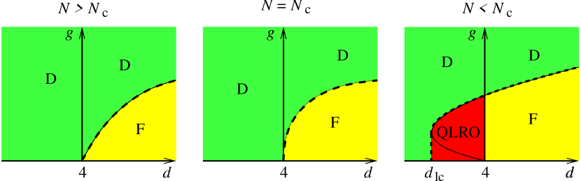
Figure 13: Phase diagram of the RF non-linear sigma model. D $=$ disordered, F $=$ ferromagnetic, QLRO $=$ quasi long-range order. Reprinted from [44].

The complete analysis [44] shows that there is a critical value of $N$, $N_{c}=2.8347408$, below which the lower critical dimension $d_{\mathrm{lc}}$ of the quasi-ordered phase plunges below $d=4$. Hence there are now two fixed points below $d=4$. For $N>N_{c}$ a ferromagnetic phase exists with lower critical dimension $d_{\mathrm{lc}}=4$. For $N<N_{c}$ one finds an expansion:

$$d_{\mathrm{lc}}^{\mathrm{RF}}=4-\epsilon_{c}\approx 4-0.1268(N-N_{c})^{2}+O((N-N_{c})^{3})\ .$$ (63)

One can also compute the exponents of the correlation function

$$\overline{S_{q}S_{-q}}\sim q^{-4+\bar{\eta}}\ ,$$ (64)

and once the fixed point is known, $\bar{\eta}$ is given by $\bar{\eta}=\epsilon-(N-1)R^{\prime\prime}(0)+{\textstyle\frac{3N-2}{8}}R^{\prime\prime\prime}(0^{+})^{2}$. There is a similar exponent for the connected thermal correlation $\eta$. Another fixed point describing magnets with random anisotropies (i.e. disorder coupling linearly to $S_{i}(x)S_{j}(x)$) is studied in [42, 43, 44, 48].

In this context, the existence of a quasi-ordered phase for the random-field XY model in $d=3$ (the scalar version of the Bragg glas) has been questioned [45]. Corrections in (63) seem to be small and at first sight exclude the quasi-ordered phase in $d=3$. This should however be taken with a (large) grain of salt [49]. Indeed the above model does not even contain topological defects (i.e. vortices) as it was directly derived in the continuum. In the absence of topological defects it is believed that the lower critical dimension is $d_{\mathrm{lc}}=2$ (with logarithmic corrections there). Hence the above series should converge to that value for $N=2$, indicating higher order corrections to (63). Another analysis [50] based on a FRG on the soft-spin model, which may be able to capture vortices, indicates $d_{\mathrm{lc}}(N=2)>3$. Unfortunately, it uses a truncation of FRG which cannot be controlled perturbatively, and as a result, does not match the 2-loop result. It would be interesting to construct a better approximation which predicts accurately at which dimension the soft and hard spin model differ in their lower critical dimensions, probably when vortices become unbound due to disorder.

19 More universal distributions

Figure 14: Scaling function $\Phi(z)$ for the ($1+1$)–dimensional harmonic model, compared to the Gaussian approximation for $\zeta=1.25$. Data from [51].

As we have already seen, exponents are not the only interesting quantities: In experiments and simulations, often whole distributions can be measured, as e.g. the universal width distribution of an interface that we have computed at depinningc [51, 52]. Be $\left<u\right>$ the average position of an interface for a given disorder configuration, then the spatially averaged width

$$w^{2}:=\frac{1}{L^{d}}\int_{x}\left(u(x)-\left<u\right>\right)^{2}$$ (65)

is a random variable, and we can try to calculate and measure its distribution $P(w^{2})$. The rescaled function $\Phi(z)$, defined by

$$P(w^{2})={1}/{\overline{w^{2}}}\,\Phi\left({w^{2}}/{\overline{w^{2}}}\right)$$ (66)

will be universal, i.e. independent of microscopic details and the size of the system.

Supposing all correlations to be Gaussian, $\Phi(z)$ can be calculated analytically. It depends on two parameters, the roughness exponent $\zeta$ and the dimension $d$. Numerical simulations displayed on figure 14 show spectacular agreement between analytical and numerical results. As expected, the Gaussian approximation is not exact, but to see deviations in a simulation, about $10^{5}$ samples have to be used. Analytically, corrections can be calculated: They are of order $R^{\prime\prime\prime}(0^{+})^{4}$ and small. Physically, the distribution is narrower than a Gaussian.

There are more observables of which distributions have been calculated within FRG, or measured in simulations. Let us mention fluctuations of the elastic energy [53], and of the depinning force [54, 55].

20 Anisotropic depinning, directed percolation, branching and all that

Figure 15: The diagram generating the irreversible nonlinear KPZ term with one disorder vertex and one $c_{4}$ vertex (the bars denote spatial derivatives).

We have discussed in section 16 isotopic depinning, which as the name suggests is a situation, where the system is invariant under a tilt. This isotropy can be broken through an additional anharmonic elasticity

$$E_{\mathrm{elastic}}=\int_{x}\frac{1}{2}\left[\nabla u(x)\right]^{2}+c_{4}\left[\nabla u(x)\right]^{4}\ ,$$ (67)

leading to a drastically different universality class, the so-called anisotropic depinning universality class, as found recently in numerical simulations [56]. It has been observed in simulations [57, 58], that the drift-velocity of an interface is increased, which can be interpreted as a tilt-dependent term, leading to the equation of motion in the form

$$\partial_{t}u(x,t)=\nabla^{2}u(x,t)+\lambda\left[\nabla u(x,t)\right]^{2}+F(x,u(x,t))+f\ .$$ (68)

However it was for a long time unclear, how this new term (proportional to $\lambda$), which usually is referred to as a KPZ-term, is generated, especially in the limit of vanishing drift-velocity. In [59] we have shown that this is possible in a non-analytic theory, due to the diagram given in figure 15.

For anisotropic depinning, numerical simulations based on cellular automaton models which are believed to be in the same universality class [60, 61], indicate a roughness exponent $\zeta\approx 0.63$ in $d=1$ and $\zeta\approx 0.48$ in $d=2$. On a phenomenological level it has been argued [60, 61, 62] that configurations at depinning can be mapped onto directed percolation in $d=1+1$ dimensions, which yields indeed a roughness exponent $\zeta_{\mathrm{DP}}=\nu_{\perp}/\nu_{\|}=0.630\pm 0.001$, and it would be intriguing to understand this from a systematic field theory.

This theory was developed in [59], and we review the main results here. A strong simplification is obtained by going to the Cole-Hopf transformed fields

$$Z({x,t}):={\mathrm{e}}^{\lambda u(x,t)}\qquad\Leftrightarrow\qquad u(x,t)=\frac{\ln(Z(x,t))}{\lambda}\ .$$ (69)

The equation of motion becomes after multiplying with $\lambda Z(x,t)$ (dropping the term proportional to $f$)

$$\partial_{t}Z(x,t)=\nabla^{2}Z(x,t)+{{\lambda}}F\left(x,\frac{\ln(Z(x,t))}{{\lambda}}\right)Z(x,t)$$ (70)

and the dynamical action (after averaging over disorder)

$${\cal S}=\int_{xt}\tilde{Z}(x,t)\left(\partial_{t}-\nabla^{2}\right)Z(x,t)-\frac{\lambda^{2}}{2}\int_{xtt^{\prime}}\tilde{Z}(x,t){Z}(x,t)\,\Delta\!\left(\frac{\ln Z(x,t)-\ln Z(x,t^{\prime})}{\lambda}\right)\tilde{Z}(x,t^{\prime})Z(x,t^{\prime})$$ (71)

This leads to the FRG flow equation at 1-loop order

$$\partial_{\ell}\Delta(u) = (\epsilon-2\zeta)\Delta(u)+\zeta u\Delta^{\prime}(u)-\Delta^{\prime\prime}(u)\left(\Delta(u)-\Delta(0)\right)-\Delta^{\prime}(u)^{2}$$ (72)

$$+2\lambda\Delta(u)\Delta^{\prime}(0^{+})+2\lambda^{2}\left(\Delta(u)^{2}+\Delta(u)\Delta(0)\right)$$

The first line is indeed equivalent to (18) using $\Delta(u)=-R^{\prime\prime}(u)$. The second line is new and contains the terms induced by the KPZ term, i.e. the term proportional to $\lambda$ in (68).

Equation (72) possesses the following remarkable property: A three parameter subspace of exponential functions forms an exactly invariant subspace. Even more strikingly, this is true to all orders in perturbation theory [59]! The subspace in question is ($0\leq u\leq 1/\lambda$)

$$\Delta(u)=\frac{\epsilon}{\lambda^{2}}\left(a+b\,{\mathrm{e}}^{-\lambda u}+c\,{\mathrm{e}}^{\lambda u}\right)$$ (73)

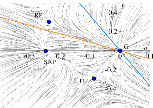
Figure 16: Fixed point structure for $\lambda=2$, which is a typical value. The ratio $c/b$ is not renormalized, see (75)-(76), such that $c/b$ is a parameter, fixed by the boundary conditions, especially $\lambda$. The fixed points are Gaussian G, Random Periodic RP (the generalization of the RP fixed point for $\lambda=0$), Self-Avoiding Polymers SAP, and Unphysical U.

The FRG-flow (72) closes in this subspace, leading to the simpler 3-dimensional flow:

$$\partial_{\ell}a = a+4a^{2}+4ac+4bc$$ (74)

$$\partial_{\ell}b = b(1+6a+b+5c)$$ (75)

$$\partial_{\ell}c = c(1+6a+b+5c)$$ (76)

This flow has a couple of fixed points, given on figure 16. They describe different physical situations. The only globally attractive fixed point is SAP, describing self-avoiding polymers. This fixed point is not attainable from the physically relevant initial conditions, which lie (as fixed point RP) between the two separatrices given on figure 16. All other fixed points are cross-over fixed points.

Figure 17: The three vertices proportional to $a$, $b$ and $c$ in equation (77).

In the Cole-Hopf representation, it is easy to see why the exponential manifold is preserved to all orders. Let us insert (73) in (71). The complicated functional disorder takes a very simple polynomial form [59].

$${\cal S}=\int_{xt}\tilde{Z}(x,t)\left(\partial_{t}-\nabla^{2}\right)Z(x,t)-\int_{x}\int_{t<t^{\prime}}\tilde{Z}(x,t)\tilde{Z}(x,t^{\prime})\left(aZ(x,t)Z(x,t^{\prime})+bZ(x,t)^{2}+cZ(x,t^{\prime})^{2}\right)\ .$$ (77)

The vertices are plotted on figure 17. It is intriguing to interpret them as particle interaction ($a$) and as different branching processes ($b$ and $c$): $Z$ destroys a particle and $\tilde{Z}$ creates one. Vertex $b$ can e.g. be interpreted as two particles coming together, annihilating one, except that the annihilated particle is created again in the future. However, if the annihilation process is strong enough, the reappearance of particles may not play a role, such that the interpretation as particle annihilation or equivalently directed percolation is indeed justified.

One caveat is in order, namely that the fixed points described above, are all transition fixed point, and nothing can a priori be said about the strong coupling regime. However this is the regime seen in numerical simulations, for which the conjecture about the equivalence to directed percolation has been proposed. Thus albeit intriguing, the above theory is only the starting point for a more complete understanding of anisotropic depinning. Probably, one needs another level of FRG, so as standard FRG is able to treat directed polymers, or equivalently the KPZ-equation in the absence of disorder.

21 Problems not treated in these notes…and perspectives

Problems not treated in these notes are too numerous to list. Let us just mention some: [63] consider depinning at the upper critical dimension. In [17], the crossover from short-ranged to long-ranged correlated disorder is treated. Our techniques can be applied to the statics at 3-loop order [64]. But many questions remain open. Some have already been raised in these notes, another is whether FRG can also be applied to other systems, as e.g. spinglasses or window glasses. Can FRG be used as a tool to go beyond mean-field or mode-coupling theories? Another open issue is the applicability of FRG beyond the elastic limit, i.e. to systems with overhangs and topological defects, non-liear elasticity [65], or to more general fractal curves than (directed) interfaces. For random periodic disorder in $d=2$, temperature is marginal, and a freezing transition can be discussed (see e.g. [66, 67]). It would be interesting to connect this to methods of conformal field theory and stochastic Löwner evolution. We have to leave these problems for future research and as a challenge for the reader to plunge deeper into the mysteries of functional renormalization.

Appendix A Derivation of the functional RG equations

In section 6, we had seen that 4 is the upper critical dimension. As for standard critical phenomena [39], we now construct an $\epsilon=(4-d)$-expansion. Taking the dimensional reduction result (12) in $d=4$ dimensions tells us that the field $u$ is dimensionless. Thus, the width $\sigma=-R^{\prime\prime}(0)$ of the disorder is not the only relevant coupling at small $\epsilon$, but any function of $u$ has the same scaling dimension in the limit of $\epsilon=0$, and might thus equivalently contribute. The natural conclusion is to follow the full function $R(u)$ under renormalization, instead of just its second moment $R^{\prime\prime}(0)$. Such an RG-treatment is most easily implemented in the replica approach: The $n$ times replicated partition function becomes after averaging over disorder

$$\overline{\exp\!\left(-\frac{1}{T}\sum_{a=1}^{n}E_{\mathrm{el}}[u_{a}]-\frac{1}{T}\sum_{a=1}^{n}{E_{\mathrm{DO}}[u_{a}]}\right)}=\exp\left(-\frac{1}{T}\sum_{a=1}^{n}{E_{\mathrm{el}}[u_{a}]}+\frac{1}{2T^{2}}\sum_{a,b=1}^{n}\int{\mathrm{d}}^{d}x\,R\Big{(}u_{a}(x)-u_{b}(x)\Big{)}\right)\ .$$ (78)

Perturbation theory is constructed along the following lines (see [23, 14] for more details.) The bare correlation function, graphically depicted as a solid line, is with momentum $k$ flowing through and replicas $a$ and $b$

$${}_{a}\parbox{40.13309pt}{\hskip 3.44444pt\includegraphics[scale={0.35}]{./figures/prop}\hskip 3.44444pt}_{b}\ =\frac{T\delta_{ab}}{k^{2}}\ .$$ (79)

The disorder vertex is

$$\stackrel{{\scriptstyle\!\!\!x}}{{\parbox{10.50238pt}{\hskip 3.44444pt\includegraphics[scale={0.35}]{./figures/Rab}\hskip 3.44444pt}_{b}^{a}}}\ =\int_{x}\sum_{a,b}R\Big{(}u_{a}(x)-u_{b}(x)\Big{)}\ .$$ (80)

The rules of the game are to find all contributions which correct $R$, and which survive in the limit of $T=0$. At leading order, i.e. order $R^{2}$, counting of factors of $T$ shows that only the terms with one or two correlators contribute. On the other hand, $\sum_{a,b}R(u_{a}-u_{b})$ has two independent sums over replicas. Thus at order $R^{2}$ four independent sums over replicas appear, and in order to reduce them to two, one needs at least two correlators (each contributing a $\delta_{ab}$). Thus, at leading order, only diagrams with two propagators survive. These are the following (noting $C(x-y)$ the Fourier transform of $1/k^{2}$):

$$\parbox{0.0pt}{\rule{0.0pt}{15.07996pt}}^{a}_{b}\!\!\stackrel{{\scriptstyle\!\!\!x\hskip 39.83368pty}}{{\parbox{42.30118pt}{\hskip 3.44444pt\includegraphics[scale={0.35}]{./figures/func2}\hskip 3.44444pt}_{b}^{a}}} = \int_{x}R^{\prime\prime}(u_{a}(x)-u_{b}(x))R^{\prime\prime}(u_{a}(y)-u_{a}(y))C(x-y)^{2}$$ (81)

$$\parbox{0.0pt}{\rule{0.0pt}{15.07996pt}}^{a}_{b}\!\!\stackrel{{\scriptstyle\!\!\!x\hskip 39.83368pty}}{{\parbox{42.30118pt}{\hskip 3.44444pt\includegraphics[scale={0.35}]{./figures/func1}\hskip 3.44444pt}_{b}^{a}}} = -\int_{x}R^{\prime\prime}(u_{a}(x)-u_{a}(x))R^{\prime\prime}(u_{a}(y)-u_{a}(y))C(x-y)^{2}\ .$$ (82)

In a renormalization program, we are looking for the divergences of these diagrams. These divergences are localized at $x=y$, which allows to approximate $R^{\prime\prime}(u_{a}(y)-u_{b}(y))$ by $R^{\prime\prime}(u_{a}(x)-u_{b}(x))$. The integral $\int_{x-y}C(x-y)^{2}=\int_{k}\frac{1}{(k^{2}+m^{2})^{2}}=\frac{m^{-\epsilon}}{\epsilon}$ (using the most convenient normalization for $\int_{k}$) is the standard 1-loop diagram from $\phi^{4}$-theory. We have chosen to regulate it in the infrared by a mass, i.e. physically by the harmonic well introduced in section 8.

Note that the following diagram also contains two correlators (correct counting in powers of temperature), but is not a 2-replica but a 3-replica sum:

$${\raisebox{-2.84526pt}{$\parbox{0.0pt}{\rule{0.0pt}{15.07996pt}}^{a}_{b}$}}\!\!\stackrel{{\scriptstyle\!\!\!x\hskip 39.83368pty}}{{\parbox{42.30118pt}{\hskip 3.44444pt\includegraphics[scale={0.35}]{./figures/func3}\hskip 3.44444pt}}}\!\!{\raisebox{-2.84526pt}{$\parbox{0.0pt}{\rule{0.0pt}{15.07996pt}}^{a}_{c}$}}\ \ .$$ (83)

Taking into account combinatorial factors, the rescaling (17) of $R$, as well as of the field $u$ (its dimension being the roughness exponent $\zeta$), we arrive at

$$-m\frac{\partial}{\partial m}R(u)=(\epsilon-4\zeta)R(u)+\zeta uR^{\prime}(u)+\frac{1}{2}R^{\prime\prime}(u)^{2}-R^{\prime\prime}(u)R^{\prime\prime}(0)\ .$$ (84)

Note that the field does not get renormalized due to the exact statistical tilt symmetry $u(x)\to u(x)+\alpha x$: The bare action (8), including the mass term, changes according to ${\cal H}^{\mathrm{bare}}[u]\to{\cal H}^{\mathrm{bare}}[u]+\delta{\cal H}[u]$, with

$$\delta{\cal H}[u]=c\int{\mathrm{d}}^{d}x\left[\nabla u(x)\alpha+\frac{1}{2}\alpha^{2}\right]+{m^{2}}\left[u(x)\alpha x+\frac{1}{2}\alpha^{2}x^{2}\right]\ .$$ (85)

To render the presentation clearer, the elastic constant $c$ set to $c=1$ in equation (8) has been introduced. The important observation is that all fields $u$ involved are large-scale variables, which are also present in the renormalized action, changing according to ${\cal H}^{\mathrm{ren}}[u]\to{\cal H}^{\mathrm{ren}}[u]+\delta H[u]$. The latter can be used to define the renormalized elastic coefficient $c^{\mathrm{ren}}$ and mass $m^{\mathrm{ren}}$. Since $\delta H[u]$ gives the change in energy both for the bare and the renormalized action with unchanged coefficients, $c^{\mathrm{ren}}\equiv c$ and $m^{\mathrm{ren}}\equiv m$, so neither elasticity nor mass changes under renormalization.

Appendix B Why is a cusp necessary in $4-\epsilon$ dimensions?

Let us present here another simple argument due to Leon Balents [68], why a cusp is a physical necessity in order to have a $\epsilon=4-d$ expansion. To this aim, consider a toy model with only one Fourier-mode $u=u_{q}$

$${\cal H}[u]=\frac{1}{2}q^{2}u^{2}+\sqrt{\epsilon}\,\tilde{V}(u)\ .$$ (86)

Since equation (18) has a fixed point of order $R(u)\sim\epsilon$ for all $\epsilon>0$, $V(u)$ scales like $\sqrt{\epsilon}$ for $\epsilon$ small and we have made this dependence explicit in (86) by using $V(u)=\sqrt{\epsilon}\tilde{V}(u)$. The only further input comes from the physics: For $L<L_{c}$, i.e. before we reach the Larkin length, there is only one minimum, as depicted in figure 18. On the other hand, for $L>L_{c}$, there are several minima. Thus there is at least one point for which

$$\frac{{\mathrm{d}}^{2}}{{\mathrm{d}}u^{2}}\,{\cal H}[u]=q^{2}+\sqrt{\epsilon}\,\tilde{V}^{\prime\prime}(u)<0\ .$$ (87)

In the limit of $\epsilon\to 0$, this is possible if and only if $\frac{1}{\epsilon}R^{\prime\prime\prime\prime}(0)$, which a priori should be finite for $\epsilon\to 0$, becomes infinite:

$$\frac{1}{\epsilon}R^{\prime\prime\prime\prime}(0)=\overline{V^{\prime\prime}(u)V^{\prime\prime}(u^{\prime})}\hskip 0.43057pt\raisebox{-4.30554pt}[0.0pt][3.44444pt]{\rule{0.43057pt}{11.84024pt}\hskip 0.86108pt}_{u=u^{\prime}}=\infty\ .$$ (88)

This argument shows that a cusp is indeed a physical necessity.

Figure 18: The toy model (86) before (left) and after (right) the Larkin-scale.

Acknowledgments

It is a pleasure to thank the organizers of IRS-2006 for the opportunity to give this lecture. The results presented here have been obtained in a series of inspiring collaborations with Leon Balents, Pascal Chauve, Andrei Fedorenko, Werner Krauth, Alan Middleton and Alberto Rosso. We also thank Dima Feldman, and Thomas Nattermann for useful discussions.

This work has been supported by ANR (05-BLAN-0099-01), and NSF (PHY99-07949).

References

- [1] K.J. Wiese, Disordered systems and the functional renormalization group: A pedagogical introduction, Acta Physica Slovaca 52 (2002) 341, cond-mat/0205116.
- [2] K.J. Wiese, The functional renormalization group treatment of disordered systems: a review, Ann. Henri Poincaré 4 (2003) 473–496, cond-mat/0302322.
- [3] P. Le Doussal, http://www.lancs.ac.uk/users/esqn/windsor04/program.htm (2004).
- [4] P. Le Doussal, http://online.kitp.ucsb.edu/online/sle06/ledoussal1/ (2006).
- [5] K.J. Wiese, http://online.kitp.ucsb.edu/online/sle06/wiese/ (2006).
- [6] S. Lemerle, J. Ferré, C. Chappert, V. Mathet, T. Giamarchi and P. Le Doussal, Domain wall creep in an Ising ultrathin magnetic film, Phys. Rev. Lett. 80 (1998) 849.
- [7] S. Moulinet, C. Guthmann and E. Rolley, Roughness and dynamics of a contact line of a viscous fluid on a disordered substrate, Eur. Phys. J. A 8 (2002) 437–43.
- [8] K.B. Efetov and A.I. Larkin, Sov. Phys. JETP 45 (1977) 1236.
- [9] A.I. Larkin, Sov. Phys. JETP 31 (1970) 784.
- [10] G. Parisi and N. Sourlas, Random magnetic fields, supersymmetry, and negative dimensions, Phys. Rev. Lett. 43 (1979) 744–5.
- [11] F.J. Wegner and A. Houghton, Renormalization group equation for critical phenomena, Phys. Rev. A 8 (1973) 401–12.
- [12] D.S. Fisher, Interface fluctuations in disordered systems: expansion, Phys. Rev. Lett. 56 (1986) 1964–97.
- [13] P. Le Doussal, Finite temperature Functional RG, droplets and decaying Burgers turbulence, cond-mat/0605490 (2006).
- [14] P. Le Doussal, K.J. Wiese and P. Chauve, Functional renormalization group and the field theory of disordered elastic systems, Phys. Rev. E 69 (2004) 026112, cont-mat/0304614.
- [15] A.A. Middleton, P. Le Doussal and K.J. Wiese, Measuring functional renormalization group fixed-point functions for pinned manifolds, cond-mat/0606160 (2006).
- [16] L. Balents, J.P. Bouchaud and M. Mézard, The large scale energy landscape of randomly pinned objects, J. Phys. I (France) 6 (1996) 1007–20.
- [17] P. Le Doussal and K.J. Wiese, How to measure Functional RG fixed-point functions for dynamics and at depinning, cond-mat/0610525 (2006).
- [18] A. Rosso, P. Le Doussal and K.J. Wiese, Numerical calculation of the functional renormalization group fixed-point functions at the depinning transition, cond-mat/0610821 (2006).
- [19] P. Chauve, T. Giamarchi and P. Le Doussal, Creep and depinning in disordered media, Phys. Rev. B 62 (2000) 6241–67, cond-mat/0002299.
- [20] L. Balents and P. Le Doussal, Thermal fluctuations in pinned elastic systems: field theory of rare events and droplets, Annals of Physics 315 (2005) 213–303, cond-mat/0408048.
- [21] L. Balents and P. Le Doussal, Broad relaxation spectrum and the field theory of glassy dynamics for pinned elastic systems, Phys. Rev. E 69 (2004) 061107, cond-mat/0312338.
- [22] P. Le Doussal, Chaos and residual correlations in pinned disordered systems, Phys. Rev. Lett. 96 235702 (2006).
- [23] L. Balents and D.S. Fisher, Large- expansion of -dimensional oriented manifolds in random media, Phys. Rev. B 48 (1993) 5949–5963.
- [24] P. Chauve, P. Le Doussal and K.J. Wiese, Renormalization of pinned elastic systems: How does it work beyond one loop?, Phys. Rev. Lett. 86 (2001) 1785–1788, cond-mat/0006056.
- [25] S. Scheidl, Private communication about 2-loop calculations for the random manifold problem. 2000-2004.
- [26] Yusuf Dincer, Zur Universalität der Struktur elastischer Mannigfaltigkeiten in Unordnung, Master’s thesis, Universität Köln, August 1999.
- [27] P. Chauve and P. Le Doussal, Exact multilocal renormalization group and applications to disordered problems, Phys. Rev. E 64 (2001) 051102/1–27, cond-mat/0006057.
- [28] A.A. Middleton, Numerical results for the ground-state interface in a random medium, Phys. Rev. E 52 (1995) R3337–40.
- [29] P. Le Doussal and K.J. Wiese, 2-loop functional renormalization for elastic manifolds pinned by disorder in dimensions, Phys. Rev. E 72 (2005) 035101 (R), cond-mat/0501315.
- [30] M. Kardar, G. Parisi and Y.-C. Zhang, Dynamic scaling of growing interfaces, Phys. Rev. Lett. 56 (1986) 889–892.
- [31] E. Marinari, A. Pagnani and G. Parisi, Critical exponents of the KPZ equation via multi-surface coding numerical simulations, J. Phys. A 33 (2000) 8181–92.
- [32] P. Le Doussal and K.J. Wiese, Functional renormalization group at large for random manifolds, Phys. Rev. Lett. 89 (2002) 125702, cond-mat/0109204v1.
- [33] M. Mézard and G. Parisi, Replica field theory for random manifolds, J. Phys. I (France) 1 (1991) 809–837.
- [34] P. Le Doussal and K.J. Wiese, Derivation of the functional renormalization group -function at order for manifolds pinned by disorder, Nucl. Phys. B 701 (2004) 409–480, cond-mat/0406297.
- [35] T. Nattermann, S. Stepanow, L.H. Tang and H. Leschhorn, Dynamics of interface depinning in a disordered medium, J. Phys. II (France) 2 (1992) 1483–1488.
- [36] O. Narayan and D.S. Fisher, Threshold critical dynamics of driven interfaces in random media, Phys. Rev. B 48 (1993) 7030–42.
- [37] P. Le Doussal, K.J. Wiese and P. Chauve, 2-loop functional renormalization group analysis of the depinning transition, Phys. Rev. B 66 (2002) 174201, cond-mat/0205108.
- [38] K.J. Wiese, Supersymmetry breaking in disordered systems and relation to functional renormalization and replica-symmetry breaking, J. Phys. A 17 (2005) S1889–S1898, cond-mat/0411656.
- [39] J. Zinn-Justin, Quantum Field Theory and Critical Phenomena, Oxford University Press, Oxford, 1989.
- [40] J. Kurchan, Supersymmetry in spin glass dynamics, J. Phys. I France 2 (1992) 1333.
- [41] D.S. Fisher, Random fields, random anisotropies, nonlinear sigma models and dimensional reduction, Phys. Rev. B 31 (1985) 7233–51.
- [42] D.E. Feldman, Quasi-long-range order in the random anisotropy Heisenberg model: Functional renormalization group in 4- epsilon dimensions, Phys. Rev. B 61 (2000) 382–90.
- [43] D.E. Feldman, Critical exponents of the random-field -model, cond-mat/0010012 (2000).
- [44] P. Le Doussal and K.J. Wiese, Random field spin models beyond one loop: a mechanism for decreasing the lower critical dimension, Phys. Rev. Lett. 96 (2006) 197202, cond-mat/0510344.
- [45] G. Tarjus and M. Tissier, A unified picture of ferromagnetism, quasi-long range order and criticality in random field models, Phys. Rev. Lett. 96 (2006) 087202, cond-mat/0511096.
- [46] G. Tarjus and M. Tissier, Two-loop functional renormalization group of the random field and random anisotropy models, cond-mat/0606698 (2006).
- [47] T. Giamarchi and P. Le Doussal, Elastic theory of flux lattices in the presence of weak disorder, Phys. Rev. B 52 (1995) 1242–70.
- [48] F. Kühnel, P. Le Doussal and K.J. Wiese, unpublished 2006.
- [49] P. Le Doussal, Talk at IHEP, Conference “Renormalization non-perturbative : de la physique de la matière condensée à la cosmologie”, Feb. 2006.
- [50] G. Tarjus and M. Tissier, Nonperturbative functional renormalization group for random-field models: The way out of dimensional reduction, Phys. Rev. Lett. 93 (2004) 267008.
- [51] A. Rosso, W. Krauth, P. Le Doussal, J. Vannimenus and K.J. Wiese, Universal interface width distributions at the depinning threshold, Phys. Rev. E 68 (2003) 036128, cond-mat/0301464.
- [52] P. Le Doussal and K.J. Wiese, Higher correlations, universal distributions and finite size scaling in the field theory of depinning, Phys. Rev. E 68 (2003) 046118, cond-mat/0301465.
- [53] A. Fedorenko and S. Stepanow, Universal energy distribution for interfaces in a random-field environment, Phys. Rev. E 67 (2003) 056115.
- [54] A. Fedorenko, P. Le Doussal and K.J. Wiese, Universal distribution of threshold forces at the depinning transition, Phys. Rev. E 74 (2006) 041110.
- [55] C.J. Bolech and A. Rosso, Universal statistics of the critical depinning force of elastic systems in random media, Phys. Rev. Lett. 93 (2004) 125701, cond-mat/0403023.
- [56] A. Rosso and W. Krauth, Origin of the roughness exponent in elastic strings at the depinning threshold, Phys. Rev. Lett. 87 (2001) 187002.
- [57] L.A.N. Amaral, A. L. Barabasi and H.E. Stanley, Critical dynamics of contact line depinning, Phys. Rev. Lett. 73 (1994).
- [58] L.-H. Tang, M. Kardar and D. Dhar, Driven depinning in anisotropic media, Phys. Rev. Lett. 74 (1995) 920–3.
- [59] P. Le Doussal and K.J. Wiese, Functional renormalization group for anisotropic depinning and relation to branching processes, Phys. Rev. E 67 (2003) 016121, cond-mat/0208204.
- [60] L.-H. Tang and H. Leschhorn, Pinning by directed percolation, Phys. Rev. A 45 (1992) R8309–12.
- [61] S.V. Buldyrev, A.-L. Barabasi, F. Caserta, S. Havlin, H.E. Stanley and T. Vicsek, Anomalous interface roughening in porous media: experiment and model, Phys. Rev. A 45 (1992) R8313–16.
- [62] S.C. Glotzer, M.F. Gyure, F. Sciortino, A. Coniglio and H.E. Stanley, Pinning in phase-separating systems, Phys. Rev. E 49 (1994) 247–58.
- [63] A. Fedorenko and S. Stepanow, Depinning transition at the upper critical dimension, Phys. Rev. E 67 (2003) 057104, cond-mat/0209171.
- [64] K.J. Wiese and P. Le Doussal, 3-loop FRG study of pinned manifolds, in preparation.
- [65] P. Le Doussal, K.J. Wiese, E. Raphael and Ramin Golestanian, Can non-linear elasticity explain contact-line roughness at depinning?, Phys. Rev. Lett. 96 (2006) 015702, cond-mat/0411652.
- [66] D. Carpentier and P. Le Doussal, Disordered xy models and coulomb gases: renormalization via traveling waves, Phys. Rev. Lett. 81 (1998) 2558–61.
- [67] G. Schehr, Free Fermions, Functional RG and the Cardy Ostlund fixed line at low temperature, cond-mat/0607657 (2006).
- [68] L. Balents, private communication.