Nonlocal Andreev reflection at high transmissions

Abstract

We analyze non-local effects in electron transport across three-terminal normal-superconducting-normal (NSN) structures. Subgap electrons entering S-electrode from one N-metal may form Cooper pairs with their counterparts penetrating from another N-metal. This phenomenon of crossed Andreev reflection – combined with normal scattering at SN interfaces – yields two different contributions to non-local conductance which we evaluate non-perturbatively at arbitrary interface transmissions. Both these contributions reach their maximum values at fully transmitting interfaces and demonstrate interesting features which can be tested in future experiments.

At sufficiently low temperatures Andreev reflection (AR) And dominates charge transfer through an interface between a normal metal and a superconductor (NS): An electron propagating from the normal metal with energy below the superconducting gap $\Delta$ enters the superconductor at a length of order of the superconducting coherence length $\xi$, forms a Cooper pair together with another electron, while a hole goes back into the normal metal. As a result, the net charge $2e$ is transferred through the NS interface which acquires non-zero subgap conductance BTK .

In hybrid NSN structures with two N-terminals, electrons may penetrate into a superconductor through both NS interfaces. Provided the superconductor size (distance between two NS interfaces) $L$ strongly exceeds $\xi$, AR processes at these interfaces are independent. If, however, the distance $L$ is smaller than or comparable with $\xi$, two additional non-local processes come into play (see Fig. 1). Firstly, an electron with subgap energy propagating from one N-metal can penetrate through the superconductor into another N-electrode with the probability $\sim\exp(-L/\xi)$. Secondly, an electron penetrating into the superconductor from the first N-terminal may form a Cooper pair by “picking up” another electron from the second N-terminal. In this case a hole will go into the second (not the first!) N-metal and, hence, AR turns into a non-local effect. The probability of this process – usually called crossed Andreev reflection (CAR) BF ; GF – also decays as $\sim\exp(-L/\xi)$ and, in combination with direct electron transfer between normal electrodes, determines non-local conductance in hybrid multi-terminal structures which can be directly measured in experiment.

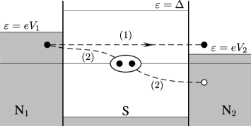
Figure 1: Two elementary processes contributing to non-local conductance of an NSN device: (1) direct electron transfer and (2) crossed Andreev reflection.

CAR has recently become a subject of intensive investigations both in experiment Beckmann ; Teun ; Venkat and in theory FFH ; Fabio ; Melin ; Belzig ; BG (see also further references therein). Although a non-local conductance was observed in all these experiments, an unambiguous and detailed interpretation of the existing experimental data still remains a challenge, to a certain extent because in addition to the above processes a number of other physical effects may considerably influence the observations. Among such effects we mention, e.g, charge imbalance (relevant close to the superconducting critical temperature Beckmann ; Venkat ) as well as zero-bias anomalies in the Andreev conductance due to both disorder-enhanced interference of electrons VZK ; HN ; Z and Coulomb effects Z ; HHK ; GZ06 . CAR is also sensitive to magnetic properties of normal electrodes. Although theoretical investigation of the above physical effects is certainly of interest and may help to account for some experimental observations, we believe that, beforehand, it is important to reach quantitative understanding of CAR in simpler situations when (at least some of) the above effects can be disregarded.

As in most cases metallic interfaces are not fully transparent, AR is usually combined with normal electron scattering at such interfaces. The relative “weights” of these two processes are determined by interface transmission. In the case of multi-terminal hybrid structures normal reflection, tunneling, local AR and CAR combine in a complicated and non-trivial manner. For instance, it was demonstrated FFH ; Fabio that in the lowest order in the interface barrier transmission and at $T=0$ CAR contribution to cross-terminal conductance is exactly cancelled by that from elastic electron cotunneling FN , while no such cancellation is expected in higher orders in the transmission Melin . However, complete theory of non-local phenomena in question which would fully describe an interplay between all scattering processes to all orders in the interface transmissions and set the maximum scale of the effect remains unavailable. Such a theory requires non-perturbative methods and is the main subject of the present work.

Figure 2: Schematics of our NSN device.

The model and formalism. Consider three-terminal NSN structure depicted in Fig. 2. We will assume that all three metallic electrodes are non-magnetic and ballistic, i.e. the electron elastic mean free path is large. Transmissions $D_{1}$ and $D_{2}$ of two SN interfaces (with cross-sections ${\cal A}_{1}$ and ${\cal A}_{2}$) may take any value from zero to one. The distance between the two interfaces $L$ as well as other geometric parameters are assumed to be much larger than $\sqrt{{\cal A}_{1,2}}$, i.e. effectively both contacts are metallic constrictions. In this case the voltage drops only across SN interfaces and not inside large metallic electrodes. Hence, nonequilibrium (e.g. charge imbalance) effects related to the electric field penetration into the S-electrode can be neglected. In what follows we will also ignore Coulomb effects Z ; HHK ; GZ06 .

For convenience, we will set the electric potential of the S-electrode equal to zero, $V=0$. In the presence of bias voltages $V_{1}$ and $V_{2}$ applied to two normal electrodes (see Fig. 2) the currents $I_{1}$ and $I_{2}$ will flow through SN₁ and SN₂ interfaces. These currents can be evaluated with the aid of the quasiclassical formalism of nonequilibrium Green-Eilenberger-Keldysh functions $\hat{g}^{R,A,K}$ BWBSZ . In the ballistic limit the corresponding equations take the form

$$\begin{split}\left[\varepsilon\hat{\tau}_{3}+eV(\bm{r},t)-\hat{\Delta}(\bm{r},t),\hat{g}^{R,A,K}(\bm{p}_{F},\varepsilon,\bm{r},t)\right]+\\ +i\bm{v}_{F}\nabla\hat{g}^{R,A,K}(\bm{p}_{F},\varepsilon,\bm{r},t)=0,\end{split}$$ (1)

where $[\hat{a},\hat{b}]=\hat{a}\hat{b}-\hat{b}\hat{a}$, $\varepsilon$ is the quasiparticle energy, $\bm{p}_{F}=m\bm{v}_{F}$ is the electron Fermi momentum vector and $\hat{\tau}_{3}$ is the Pauli matrix. The functions $\hat{g}^{R,A,K}$ also obey the normalization conditions $(\hat{g}^{R})^{2}=(\hat{g}^{A})^{2}=1$ and $\hat{g}^{R}\hat{g}^{K}+\hat{g}^{K}\hat{g}^{A}=0$. Here and below the product of matrices is defined as time convolution.

The matrices $\hat{g}$ and $\hat{\Delta}$ have the standard form

$$\hat{g}^{R,A,K}=\begin{pmatrix}g^{R,A,K}&f^{R,A,K}\\ \tilde{f}^{R,A,K}&\tilde{g}^{R,A,K}\\ \end{pmatrix},\quad\hat{\Delta}=\begin{pmatrix}0&\Delta\\ -\Delta^{*}&0\\ \end{pmatrix},$$ (2)

where $\Delta$ is the BCS order parameter. The current density is related to the Keldysh function $\hat{g}^{K}$ as

$$\bm{j}(\bm{r},t)=-\dfrac{eN_{0}}{4}\int d\varepsilon\left<\bm{v}_{F}\mathrm{Sp}[\hat{\tau}_{3}\hat{g}^{K}(\bm{p}_{F},\varepsilon,\bm{r},t)]\right>,$$ (3)

where $N_{0}=mp_{F}/2\pi^{2}$ is the density of state at the Fermi level and angular brackets $\left<...\right>$ denote averaging over the Fermi momentum directions.

The above equations should be supplemented by appropriate boundary conditions. In order to match quasiclassical Green functions at the N- and S-sides of SN₁ interface (respectively $\check{g}_{N_{1}}$ and $\check{g}_{S}$) we will make use of Zaitsev boundary conditions Zaitsev for matrices $\check{g}=\left(\begin{smallmatrix}\hat{g}^{R}&\hat{g}^{K}\\ 0&\hat{g}^{A}\end{smallmatrix}\right)$:

$$\check{g}^{a}=\check{g}_{N_{1}}^{+}-\check{g}_{N_{1}}^{-}=\check{g}_{S}^{+}-\check{g}_{S}^{-},$$ (4)

$$\check{g}^{a}[R_{1}(\check{g}^{+})^{2}+(\check{g}^{-})^{2}]=D_{1}\check{g}^{-}\check{g}^{+},$$ (5)

where $\check{g}^{\pm}=\check{g}_{N_{1}}^{+}+\check{g}_{N_{1}}^{-}\pm\check{g}_{S}^{+}\pm\check{g}_{S}^{-}$, $\check{g}_{S}^{\pm}=\check{g}_{S}(\pm p_{x})$ (see Fig. 3a), $R_{1}(p_{x_{1}})\equiv 1-D_{1}(p_{x_{1}})$, $p_{x_{1}}$ is the component of $\bm{p}_{F}$ normal to the SN₁ interface. Green functions at SN₂ interface are matched analogously. Deep inside metallic electrodes S, N₁ and N₂ the Green functions should approach their equilibrium values $\hat{g}^{R,A}=\pm(\varepsilon\hat{\tau}_{3}-\hat{\Delta})/\Omega^{R,A}$ in a superconductor and $\hat{g}^{R,A}=\pm\hat{\tau}_{3}$ in normal metals, $\Omega^{R,A}=\sqrt{(\varepsilon\pm i\delta)^{2}-\Delta^{2}}$. For the Keldysh functions far from interfaces we have $\hat{g}^{K}=\hat{g}^{R}\left(\begin{smallmatrix}h_{+}&0\\ 0&h_{-}\end{smallmatrix}\right)-\left(\begin{smallmatrix}h_{+}&0\\ 0&h_{-}\end{smallmatrix}\right)\hat{g}^{A}$, where $h_{\pm}=\tanh[(\epsilon\pm eV)/2T]$. Voltage in above expression equals to $V=0$, $V_{1}$ and $V_{2}$ respectively in S, N₁ and N₂ electrodes. The parameter $\Delta$ is chosen to be real.

Figure 3: Quasiclassical trajectories contributing to local (a) and non-local (b and c) currents.

Relevant trajectories. Electron trajectories which contribute to the current $I_{1}$ through SN₁interface are shown in Fig. 3. Trajectories presented in Fig. 3a do not enter the terminal N₂ and yield the standard BTK contribution BTK to $I_{1}$. In addition there exist trajectories (Fig. 3b,c) involving all three electrodes. They fully account for all scattering processes – both normal and AR – to all orders in the interface transmissions and determine non-local conductance of our NSN device. As follows from Fig. 3b,c for each direction of $p_{x}$ one can distinguish four different contributions to non-local conductance corresponding to different trajectory combinations.

Note that applicability of the above quasiclassical formalism with boundary conditions (5) to hybrid structures with two (or more) barriers is, in general, a non-trivial issue GZ02 which requires a comment. Electrons scattered at different barriers may interfere and form bound states (resonances) which cannot be correctly described within a formalism employing Zaitsev boundary conditions Zaitsev . In our geometry, however, any relevant trajectory reaches each interface only once whereas the probability of multiple reflections at both interfaces is small in the parameter ${\cal A}_{1}{\cal A}_{2}/L^{4}\ll 1$. Hence, resonances formed by multiply reflected electron waves can be neglected, and our formalism remains adequate for the problem in question.

Quasiclassical Green functions. The above equations can be conveniently solved introducing parameterization of the matrix Green functions $\hat{g}^{R,A,K}$ by four Riccati amplitudes and two “distribution functions” Eschrig . This parameterization allows to transform Eq. (1) to a set of decoupled equations. It is also important that non-linear Zaitsev boundary conditions (4), (5) can be rewritten in terms of Riccati amplitudes and “distribution functions” in a rather simple form Eschrig . Integration of the resulting equations along the trajectories shown in Fig. 3 is straightforward. Finally we arrive at the following expression for the Keldysh Green function $g^{K}_{N_{1}}$ at SN₁ interface (on the N-metal side)

$$g_{N_{1}}^{K}=g_{1,a}^{K}(V_{1})+g_{1,b+c}^{K}(V_{1})+g_{12,b+c}^{K}(V_{2}).$$ (6)

Here $g_{1,a}^{K}(V_{1})$ comes from the trajectories of Fig. 3a responsible for the BTK current at SN₁ interface, while two other terms come from the trajectories of Fig. 3b,c which also involve N₂-electrode. The term $g_{1,b+c}^{K}(V_{1})$ yields a correction to the BTK term which will be discussed later. The last contribution $g_{12,b+c}^{K}(V_{2})$ accounts for non-local conductance of our device. For positive $p_{x_{1}}>0$ we have

$$g^{K}_{12,b+c}(V_{2})=2D_{1}D_{2}\dfrac{1-\tanh^{2}iL\Omega/v_{F}}{P(R_{1},R_{2})}\\ \times\Biggl{(}\theta_{c}R_{1}R_{2}|a|^{4}\tanh\dfrac{\varepsilon+eV_{2}}{2T}+\theta_{b}R_{2}|a|^{2}\tanh\dfrac{\varepsilon-eV_{2}}{2T}\\ +\theta_{c}R_{1}|a|^{2}\tanh\dfrac{\varepsilon-eV_{2}}{2T}+\theta_{b}\tanh\dfrac{\varepsilon+eV_{2}}{2T}\Biggr{)},$$ (7)

where we defined $\Omega\equiv\Omega^{R}$, $P(R_{1},R_{2})=|1-R_{1}R_{2}a^{2}-Q[\varepsilon(1+R_{1}R_{2}a^{2})+\Delta a(R_{1}+R_{2})]|^{2},$ $Q=\Omega^{-1}\tanh iL\Omega/v_{F}$, $a=(\Omega-\varepsilon)/\Delta$, $\theta_{b}$ and $\theta_{c}$ equal to unity for trajectories of respectively Fig. 3b and 3c and to zero otherwise. As expected, Eq. (7) identifies four different contributions entering with the corresponding amplitudes and reflection coefficients. Note that only one out of these contributions survives in the case of reflectionless interfaces. In contrast, for weakly transmitting barriers ($R_{1,2}\to 1$) and $\varepsilon<\Delta$ all four terms enter with equal prefactors.

As for the function $\tilde{g}^{K}$, at SN₁ interface it does not depend on $V_{2}$ for positive $p_{x_{1}}>0$. The values of $g^{K}$ and $\tilde{g}^{K}$ for negative $p_{x_{1}}<0$ are easily recovered by means of the relation $g^{K}(-\bm{p}_{F},-\varepsilon,\bm{r},t)=\tilde{g}^{K}(\bm{p}_{F},\varepsilon,\bm{r},t)$.

Non-local conductance. Substituting the results (6), (7) into Eq. (3) we obtain

$$I_{1}=I_{11}(V_{1})+I_{12}(V_{2}),$$ (8)

$$I_{2}=I_{21}(V_{1})+I_{22}(V_{2}).$$ (9)

Here $I_{11}$ and $I_{22}$ consist of the standard BTK currents BTK ; Zaitsev and CAR terms to be specified later and

$$I_{12}(V)=I_{21}(V)=-\frac{G_{N_{12}}}{2e}\int d\varepsilon\left[\tanh\dfrac{\varepsilon+eV}{2T}-\tanh\dfrac{\varepsilon}{2T}\right]\\ \times(1-{\cal R}_{1}|a|^{2})(1-{\cal R}_{2}|a|^{2})\dfrac{1-\tanh^{2}iL\Omega/v_{F}}{P({\cal R}_{1},{\cal R}_{2})},$$ (10)

where ${\cal D}_{1,2}\equiv 1-{\cal R}_{1,2}=D_{1,2}(p_{F}\gamma_{1,2})$ and $p_{F}\gamma_{1(2)}$ is normal to the first (second) interface component of the Fermi momentum for electrons propagating straight between the interfaces,

$$G_{N_{12}}=\frac{8\gamma_{1}\gamma_{2}{\cal N}_{1}{\cal N}_{2}{\cal D}_{1}{\cal D}_{2}}{R_{q}p_{F}^{2}L^{2}}$$ (11)

is the non-local conductance in the normal state, ${\cal N}_{1,2}=p_{F}^{2}{\cal A}_{1,2}/4\pi$ define the number of conducting channels of the corresponding interface, $R_{q}=2\pi/e^{2}$ is the quantum resistance unit. Eq. (10) represents the central result of our paper. This expression fully determines non-local conductances of our NSN device at arbitrary transmissions of SN interfaces.

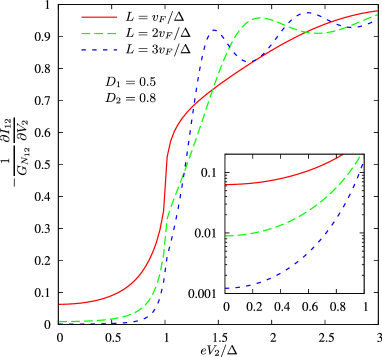
Figure 4: (Color online) Differential non-local conductance at $T=0$ as a function of voltage for $D_{1}=0.5$, $D_{2}=0.8$ and different $L$. Inset: the same for $eV<\Delta$.

The differential non-local conductance evaluated with the aid of Eq. (10) at $T=0$ is presented in Fig. 4 at sufficiently high interface transmissions. We observe that this quantity increases sharply around $eV\sim\Delta$ and approaches the $L$-independent (normal) limit at $eV\gg\Delta$. In the limit $T,V_{1,2}\ll\Delta$ only subgap quasiparticles contribute and the differential conductance becomes voltage-independent. We have $I_{12}=-G_{12}V_{2}$, where

$$\frac{G_{12}}{G_{N_{12}}}=\dfrac{{\cal D}_{1}{\cal D}_{2}(1-\tanh^{2}L\Delta/v_{F})}{[1+{\cal R}_{1}{\cal R}_{2}+({\cal R}_{1}+{\cal R}_{2})\tanh L\Delta/v_{F}]^{2}}.$$ (12)

The value $G_{12}$ (12) gets strongly suppressed with decreasing ${\cal D}_{1,2}$ and increasing $L$, as also seen in Fig. 4. Note, that the dependence of $G_{12}$ on $L$ reduces to purely exponential at all $L$ only in the lowest nonvanishing order in the transmission of at least one of the barriers, e.g., $G_{12}\propto{\cal D}_{1}^{2}{\cal D}_{2}^{2}\exp(-2L\Delta/v_{F})$ for ${\cal D}_{1,2}\ll 1$, whereas in general this dependence is slower than exponential at smaller $L$ and approaches the latter only at large $L\gg v_{F}/\Delta$.

For a given $L$ the non-local conductance reaches its maximum in the case of reflectionless interfaces $D_{1,2}=1$. Interestingly, in this case for small $L\ll v_{F}/\Delta$ the conductance $G_{12}$ identically coincides with its normal state value $G_{N_{12}}$ at any temperature and voltage. This result can easily be understood bearing in mind that for $D_{1,2}=1$ only trajectories indicated by horizontal lines in Fig. 3b,c contribute to $G_{12}$. For $L\to 0$ there is “no space” for CAR to develop on these trajectories and, hence, CAR contribution to $G_{12}$ vanishes, whereas direct transfer of electrons between N₁ and N₂ remains unaffected by superconductivity in this limit.

The situation changes provided at least one of the transmissions is smaller than one. In this case scattering at SN interfaces mixes up trajectories connecting N₁ and N₂ terminals with ones going deep into and coming from the superconductor. As a result, CAR contribution to $G_{12}$ does not vanish even in the limit $L\to 0$ and $G_{12}$ turns out to be smaller than $G_{N_{12}}$.

Finally, we would like to briefly address the non-local correction to $G_{11}$ which arises from the CAR process described by the term $g_{1,b+c}^{K}(V_{1})$ in Eq. (6). At $T,V_{1,2}\ll\Delta$ we have $I_{11}=G_{11}V_{1}$, where $G_{11}=G_{1}^{BTK}+\delta G_{11}.$ Here $G_{1}^{BTK}$ is the standard BTK term

$$G_{1}^{BTK}=\frac{8{\cal N}_{1}}{R_{q}}\left<\frac{|v_{x_{1}}|}{v_{F}}\dfrac{D^{2}_{1}(p_{x_{1}})}{[1+R_{1}(p_{x_{1}})]^{2}}\right>,$$ (13)

and for the non-local term we obtain

$$\dfrac{\delta G_{11}}{G_{N_{12}}}=\dfrac{2(1+{\cal R}_{2})(1-\tanh^{2}L\Delta/v_{F})}{[1+{\cal R}_{1}{\cal R}_{2}+({\cal R}_{1}+{\cal R}_{2})\tanh L\Delta/v_{F}]^{2}}\\ +\dfrac{{\cal D}_{1}\left[(1+{\cal R}_{2}\tanh L\Delta/v_{F})^{2}+3({\cal R}_{2}+\tanh L\Delta/v_{F})^{2}\right]}{{\cal D}_{2}[1+{\cal R}_{1}{\cal R}_{2}+({\cal R}_{1}+{\cal R}_{2})\tanh L\Delta/v_{F}]^{2}}.$$ (14)

As compared to the BTK conductance (13) the CAR correction (14) contains an extra small factor ${\cal A}_{2}/L^{2}$ and, hence, in many cases can be neglected. On the other hand, since CAR involves tunneling of one electron through each interface, for small $D_{1}\ll 1$ and $D_{2}\approx 1$ we have $\delta G_{11}\propto{\cal D}_{1}$, i.e. for $D_{1}<({\cal A}_{2}/L^{2})\exp(-2L\Delta/v_{F})$ the CAR contribution (14) may well exceed the BTK term $G_{1}^{BTK}\propto D_{1}^{2}$.

In summary, we have developed a theory of non-local electron transport in ballistic NSN structures with arbitrary interface transmissions. Non-trivial interplay between normal scattering, local and non-local Andreev reflection at SN interfaces yields a number of interesting properties of non-local conductance which can be tested in future experiments.

We would like to thank V. Chandrasekhar for communicating the results Venkat to us prior to publication and to A.A. Golubov for useful discussions at an early stage of this work.

References

- (1) A.F. Andreev, Zh. Eksp. Teor. Fiz. 46, 1823 (1964) [Sov. Phys. JETP 19, 1228 (1964)].
- (2) G.E. Blonder, M. Tinkham, and T.M. Klapwijk, Phys. Rev. B 25, 4515 (1982).
- (3) J.M. Byers and M.E. Flatte, Phys. Rev. Lett. 74, 306 (1995).
- (4) G. Deutscher and D. Feinberg, Appl. Phys. Lett. 76, 487 (2000).
- (5) D. Beckmann, H.B. Weber, and H. v. Löhneysen, Phys. Rev. Lett. 93, 197003 (2004); D. Beckmann and H. v. Löhneysen, cond-mat/0609766.
- (6) S. Russo et al., Phys. Rev. Lett. 95, 027002 (2005).
- (7) P. Cadden-Zimansky and V. Chandrasekhar, Phys. Rev. Lett. 97 (2006) 237003.
- (8) G. Falci, D. Feinberg, and F.W.J. Hekking, Europhys. Lett. 54, 255 (2001).
- (9) G. Bignon et al., Europhys. Lett. 67, 110 (2004).
- (10) R. Melin and D. Feinberg, Phys. Rev. B 70, 174509 (2004); R. Melin, Phys. Rev. B 73, 174512 (2006).
- (11) J.P. Morten, A. Brataas, and W. Belzig, cond-mat/0606561.
- (12) A. Brinkman and A.A. Golubov, cond-mat/0611144.
- (13) A.F. Volkov, A.V. Zaitsev, and T.M. Klapwijk, Physica C 210, 21 (1993).
- (14) F.W.J. Hekking and Yu.V. Nazarov, Phys. Rev. Lett. 71, 1625 (1993).
- (15) A.D. Zaikin, Phyica B 203, 255 (1994).
- (16) A. Huck, F.W.J. Hekking, and B. Kramer, Europhys. Lett. 41, 201 (1998).
- (17) A.V. Galaktionov and A.D. Zaikin, Phys. Rev. B 73, 184522 (2006).
- (18) The term “electron cotunneling” remains relevant only in the tunneling limit loosing its meaning as soon as one goes beyond perturbation theory and includes processes to all orders in barrier transmissions.
- (19) For a review see, e.g., W. Belzig et al., Superlatt. Microstruct. 25, 1251 (1999).
- (20) A.V. Zaitsev, Sov. Phys. JETP 59, 1015 (1984).
- (21) See, e.g., A.V. Galaktionov and A.D. Zaikin, Phys. Rev. B 65, 184507 (2002); M. Ozana and A. Shelankov, Phys. Rev. B 65, 014510 (2002).
- (22) M. Eschrig, Phys. Rev. B 61, 9061 (2000).