Force balance of particles trapped at fluid interfaces

Abstract

We study the effective forces acting between colloidal particles trapped at a fluid interface which itself is exposed to a pressure field. To this end we apply what we call the “force approach”, which relies solely on the condition of mechanical equilibrium and turns to be in a certain sense less restrictive than the more frequently used “energy approach”, which is based on the minimization of a free energy functional. The goals are (i) to elucidate the advantages and disadvantages of the force approach as compared to the energy approach, and (ii) to disentangle which features of the interfacial deformation and of the capillary–induced forces between the particles follow from the gross feature of mechanical equilibrium alone, as opposed to features which depend on details of, e.g., the interaction of the interface with the particles or the boundaries of the system. First, we derive a general stress–tensor formulation of the forces at the interface. On that basis we work out a useful analogy with 2D electrostatics in the particular case of small deformations of the interface relative to its flat configuration. We apply this analogy in order to compute the asymptotic decay of the effective force between particles trapped at a fluid interface, extending the validity of previous results and revealing the advantages and limitations of the force approach compared to the energy approach. It follows the application of the force approach to the case of deformations of a non–flat interface. In this context we first compute the deformation of a spherical droplet due to the electric field of a charged particle trapped at its surface and conclude that the interparticle capillary force is unlikely to explain certain recent experimental observations within such a configuration. We finally discuss the application of our approach to a generally curved interface and show as an illustrative example that a nonspherical particle deposited on an interface forming a minimal surface is pulled to regions of larger curvature.

I Introduction

Experimental evidence has been accumulated that electrically charged, $\mu$m–sized colloidal particles trapped at fluid interfaces can exhibit long–ranged attraction despite their like charges Ghezzi and Earnshaw (1997); Ruiz-García et al. (1997); Stamou et al. (2000); Quesada-Pérez et al. (2001); Nikolaides et al. (2002); Tolnai et al. (2003); Fernández-Toledano et al. (2004); Chen et al. (2005). The mechanisms leading to this attraction are not yet fully understood. An attraction mediated by the interface deformation was proposed Nikolaides et al. (2002), in analogy to the capillary force due to the weight of large floating particles Nicolson (1949); Chan et al. (1981). However, for the particles sizes used in the aforementioned experiments gravity is irrelevant. Instead, one is led to invoke electrostatic forces which act on the interface. This feature has triggered investigations of capillary deformation and capillary–induced forces beyond the well studied case of an interface simply under the effects of gravity and surface tension Megens and Aizenberg (2003); Foret and Würger (2004); Oettel et al. (2005a, b); Würger and Foret (2005); Domínguez et al. (2005); Oettel et al. (2006); Danov et al. (2006); Domínguez et al. (2007a). These studies have relied almost exclusively on what we shall call the “energy approach”, which is based on the minimization of a free energy functional obtained as a parametric function of the positions of the particles by integrating out the interfacial degrees of freedom, leading to a “potential of mean force”. This functional has to include the contribution by the interface itself, by the particles, and by the boundaries of the system. Moreover, due to technical challenges the theoretical implementation of this approach is de facto restricted to the regime of small interfacial deformations.

In the following, as an alternative we investigate the “force approach” which follows by directly applying the condition of mechanical equilibrium. Our analysis is based on the pressure field $\Pi({\bf r})$ (generated, e.g., by electrostatic forces) acting on the interface between two fluid phases. In general, the condition that an arbitrary piece ${\cal S}$ of this interface is in mechanical equilibrium reads (see, e.g., Ref. Segel, 1987)

$$\int_{\cal S}{\rm d}A\;{\bf e}_{n}\Pi+\gamma\oint_{\partial{\cal S}}{\rm d}\ell\;{\bf e}_{t}\times{\bf e}_{n}={\bf 0},$$ (1)

where ${\bf e}_{n}$ is the local unit vector normal to the interface, ${\bf e}_{t}$ is the unit vector tangent to the boundary $\partial{\cal S}$ (oriented such that ${\bf e}_{t}\times{\bf e}_{n}$ points towards the exterior of ${\cal S}$), ${\rm d}A$ is the element of the interfacial area, ${\rm d}\ell$ is the element of the arclength along the contour $\partial{\cal S}$, and $\gamma$ is the (spatially homogeneous) surface tension of the interface. In Eq. (1), the first term is the so-called bulk force exerted on the piece ${\cal S}$ by the pressure $\Pi$ and the second one is the line force exerted on the contour and generated by the surface tension (also called capillary force). This equation is the starting point for the subsequent calculations.

The force approach allows us to obtain new results, to derive previous ones more easily than within the energy approach, and to gain additional insight. This approach was employed in Ref. Kralchevsky et al., 1993 for the special case that gravity is the only relevant force and it was shown to give the same results as the energy approach if the deformations with respect to a flat interface are small everywhere. For an arbitrary pressure field acting on the interface, in Ref. Domínguez et al., 2005 we applied the force approach in order to obtain the deformation of an otherwise flat interface far from the particles generating it. In the following we further illustrate the force approach: In Sec. II we first express the force exerted by the interface in terms of a stress–tensor formulation, extending a recent result Müller et al. (2005) to the most general case $\Pi({\bf r})\neq$ constant. This formulation also allows us to establish a useful analogy between two–dimensional electrostatics and the description of small capillary deformations of a flat interface. Since this analogy has been already employed by several authors in a more or less explicit manner, here we present a thorough discussion addressing not only the issue of interfacial deformations, but also that of boundary conditions and of the capillary forces. In Sec. III we exploit the stress–tensor formulation and the electrostatic analogy in order to study the interface–mediated effective force between colloidal particles trapped at a fluid interface and to provide a detailed comparison with the corresponding results obtained within the energy approach. In Sec. IV we compute the deformation of a spherical droplet due to the presence of a charged particle at its surface, generalizing a corresponding result obtained in Ref. Domínguez et al., 2005 for a flat interface and correcting certain claims in the literature. Finally we discuss the more general case that the unperturbed interface is curved. Sec. V provides a summary and an outlook.

II Stress–tensor formulation and electrostatic analogy

The capillary force exerted by the interface (second term in Eq. (1)) can be rewritten as

$$\gamma\oint_{\partial{\cal S}}{\rm d}\ell\;{\bf e}_{t}\times{\bf e}_{n}=\mbox{}-\oint_{\partial{\cal S}}{\rm d}\ell\;({\bf e}_{t}\times{\bf e}_{n})\cdot\mathsf{T},$$ (2)

which serves to define the stress tensor $\mathsf{T}({\bf r}):=\mbox{}-\gamma\mathsf{1}({\bf r})$, where $\mathsf{1}({\bf r}\in{\cal S})$ is the 2D identity tensor on the tangent plane of ${\cal S}$ at each point ${\bf r}$. In these terms, the condition of mechanical equilibrium (Eq. (1)) takes the form

$$\int_{\cal S}{\rm d}A\;{\bf e}_{n}\Pi=\oint_{\partial{\cal S}}{\rm d}\ell\;({\bf e}_{t}\times{\bf e}_{n})\cdot\mathsf{T}.$$ (3)

We recall that ${\bf e}_{t}\times{\bf e}_{n}$ is a vector tangent to the surface ${\cal S}$ but normal to the contour $\partial{\cal S}$ and pointing outwards. This allows one to reinterpret Eq. (3) as the definition of the stress tensor $\mathsf{T}$, the flux of which through a closed boundary is the bulk force (first term in Eq. (1)) acting on the piece of interface enclosed by that boundary. In dyadic notation one has (summation over repeated indices is implied)

$$\mathsf{T}=\mbox{}-\gamma\mathsf{1}=\mbox{}-\gamma\,g^{ab}\,{\bf e}_{a}\,{\bf e}_{b}\quad\Rightarrow\quad T^{ab}=\mbox{}-\gamma\,g^{ab},$$ (4)

where $\{{\bf e}_{1},{\bf e}_{2}\}$ is a local basis, at each point tangent to the surface ${\cal S}$, and $g_{ab}={\bf e}_{a}\cdot{\bf e}_{b}$ is the induced metric ($g^{ab}$ are the contravariant components of this tensor). In this form, we have the same stress tensor as the one derived in Ref. Müller et al., 2005 using methods of differential geometry within the energy approach and for the restricted case $\Pi({\bf r})=\rm{constant}$. We remark, however, that Eq. (3) holds for an arbitrary pressure field $\Pi({\bf r})$.

An analogy with 2D electrostatics emerges by considering small deformations relative to a flat interface corresponding to the generic experimental set-up, i.e., a situation like the one in Fig. 4 but with, e.g., a charged particle Ghezzi and Earnshaw (1997); Ruiz-García et al. (1997); Aveyard et al. (2000); Quesada-Pérez et al. (2001); Tolnai et al. (2003); Fernández-Toledano et al. (2004); Chen et al. (2005), a nonspherical particle Stamou et al. (2000); Loudet et al. (2006), or a droplet at a nematic interface Smalyukh et al. (2004), so that the interface is deformed by an electric field, by a nonplanar contact line, or by the elastic stress in the nematic phase, respectively. To this end, we identify the flat interface with the $XY$–plane, so that any point of the deformed interface can be expressed as ${\bf r}={\bf r}_{\parallel}+{\bf e}_{z}u({\bf r}_{\parallel})$ with ${\bf r}_{\parallel}:=x{\bf e}_{x}+y{\bf e}_{y}$, and (the subscript _∥ will be used to denote quantities evaluated at and operators acting in the reference, flat interface)

$${\bf e}_{n}\,{\rm d}A = \left(\frac{\partial{\bf r}}{\partial x}\times\frac{\partial{\bf r}}{\partial y}\right){\rm d}y{\rm d}x=\left[{\bf e}_{z}-\nabla_{\parallel}u\right]{\rm d}A_{\parallel},$$ (5a)

$${\bf e}_{t}\,{\rm d}\ell = ({\rm d}\boldsymbol{\ell}_{\parallel}\cdot\nabla_{\parallel}){\bf r}={\rm d}\boldsymbol{\ell}_{\parallel}+{\bf e}_{z}({\rm d}\boldsymbol{\ell}_{\parallel}\cdot\nabla_{\parallel}u),$$ (5b)

where ${\rm d}\boldsymbol{\ell}_{\parallel}={\bf e}_{x}{\rm d}x+{\bf e}_{y}{\rm d}y$, ${\rm d}A_{\parallel}={\rm d}x{\rm d}y$, and $\nabla_{\parallel}={\bf e}_{x}(\partial/\partial x)+{\bf e}_{y}(\partial/\partial y)$. We denote the projection of any piece of interface ${\cal S}$ onto the $XY$–plane as ${\cal S}_{\parallel}$, and introduce the unit vector ${\bf n}$ in the $XY$–plane which is normal to the contour $\partial{\cal S}_{\parallel}$ and points outwards. With this, we expand Eq. (3) in terms of the deformation $u({\bf r}_{\parallel})$; to lowest order the component in the direction of ${\bf e}_{z}$ is linear in $u({\bf r}_{\parallel})$,

$$\int_{{\cal S}_{\parallel}}{\rm d}A_{\parallel}\;\Pi=\mbox{}-\gamma\oint_{\partial{\cal S}_{\parallel}}{\rm d}\ell_{\parallel}\;{\bf n}\cdot\nabla_{\parallel}u.$$ (6a)

The local version of this equality is the linearized Young–Laplace equation:

$$\gamma\nabla_{\parallel}^{2}u=-\Pi.$$ (6b)

To lowest order the components of Eq. (3) in the $$XY$$–plane are quadratic in the deformation:

$$\mbox{}-\int_{{\cal S}_{\parallel}}{\rm d}A_{\parallel}\;\Pi\;\nabla_{\parallel}u=\oint_{\partial{\cal S}_{\parallel}}{\rm d}\ell_{\parallel}\;{\bf n}\cdot\mathsf{T}_{\parallel},$$ (6c)

where

$$\mathsf{T}_{\parallel}\ :=\gamma\left[(\nabla_{\parallel}u)(\nabla_{\parallel}u)-\frac{1}{2}|\nabla_{\parallel}u|^{2}\;\mathsf{1}_{\parallel}\right]$$ (6d)

is a stress tensor defined in the $XY$–plane. We remark that Eq. (6c) also implies Eq. (6b) upon applying Gauss’ theorem, demonstrating consistency.

The form of Eq. (6b) allows us to identify $u$ with an electrostatic potential (and $-\nabla_{\parallel}u$ with an electric field), $\Pi$ with a charge density (“capillary charge” Kralchevsky et al. (2001)), and $\gamma$ with a permittivity. The boundary conditions usually imposed on $u$ at a contour ${\cal C}_{\parallel}$ have a close electrostatic analogy, too (see Fig. 1 for the notation):

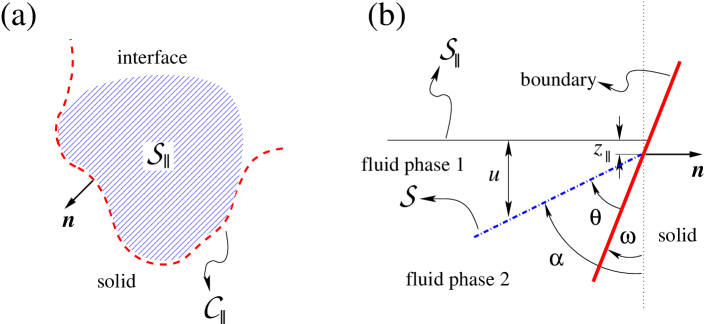
Figure 1: Generic view of the three-phase contact line of an interface with a solid boundary. (a) Top view: projection ${\cal S}_{\parallel}$ onto the $XY$-plane of the interface (dashed area) near the projected contact line ${\cal C}_{\parallel}$ (dashed line). The unit vector ${\bf n}$ is normal to the projected contact line and is directed towards the exterior of ${\cal S}_{\parallel}$. (b) Side view of the same configuration within a vertical plane containing ${\bf n}$. The thin horizontal line is the section of ${\cal S}_{\parallel}$ (i.e., the flat, unperturbed interface), while the dash–dotted line is the section of the actual interface ${\cal S}$, which can be approximated locally by the tangent forming an angle $\theta$ (contact angle) with the solid boundary. The latter is the full thick line, which looks locally like a straight line, in general inclined by an angle $\omega$ with respect to the vertical direction (dotted line). The height of the interface at contact entering into the boundary condition (7) is $z_{\parallel}:=z({\bf r}_{\parallel})$. The boundary condition (8) expresses the slope of the interface at contact with $\alpha:=\theta+\omega$.

(i) The potential is given at ${\cal C}_{\parallel}$. $\Leftrightarrow$ The interface is pinned at the contour at a height $z({\bf r}_{\parallel})$:

$$u({\bf r}_{\parallel})=z({\bf r}_{\parallel}),\qquad{\bf r}_{\parallel}\in{\cal C}_{\parallel}.$$ (7)

(ii) The normal component of the electric field is given at ${\cal C}_{\parallel}$. $\Leftrightarrow$ The contact angle $\theta({\bf r}_{\parallel})$ is specified at each point of the contour:

$$({\bf n}\cdot\nabla_{\parallel})u({\bf r}_{\parallel})=\cot\alpha({\bf r}_{\parallel}),\qquad{\bf r}_{\parallel}\in{\cal C}_{\parallel},$$ (8)

where the angle $\alpha({\bf r}_{\parallel})$, defined in Fig. 1, must be close to $\pi/2$ for reasons of consistency with the approximation of small deformations.

This means that the equivalence with the corresponding electrostatic analogy is exact concerning the relationship between the deformation field $u({\bf r}_{\parallel})$ and its sources (i.e., the pressure field $\Pi$ and the boundary conditions). The analogy carries over almost exactly, too, to the elastic forces in the $XY$–plane (“lateral capillary forces”) arising from interfacial deformation: according to Eqs. (6c, 6d), $\mathsf{T}_{\parallel}$ corresponds to Maxwell’s stress tensor, the flux of which through a closed boundary gives the electric force acting on the enclosed charge. However, the force related to the deformation is actually the interfacial stress, which is minus the flux of this tensor (see Eq. (2)). Therefore, the electrostatic analogy is valid up to a reversal of the forces and the peculiarity arises that “capillary charges” will attract (repel) each other if they have equal (different) sign. The origin of this peculiarity is that Eq. (3), which in the spirit of electrostatics can be reinterpreted as a definition of $\mathsf{T}$, is actually a relationship between bulk and capillary forces as two physically different kinds of forces. The actual connection of $\mathsf{T}$ with a force is Eq. (2).

We note that the electrostatic analogy holds wherever the deformation of the interface is small, even if there are other regions of the interface where this is not true. Such “nonlinear patches” can be surrounded by contours where the deformation is small, so that the values of the field $u$ and of its derivatives at these contours play the role of a boundary condition for the “linear patches”. This means that the “nonlinear patches” are replaced by a distribution of virtual “capillary charges” inside the corresponding regions. In particular, there is a simple physical meaning associated with the total “capillary charge” and the total “capillary dipole”. The “capillary charge” $Q$ of a piece of interface bounded by a contour ${\cal C}$ is given by Gauss’ theorem solely in terms of the value of the deformation at the contour (see Eq. (6a)):

$$Q=\mbox{}-\gamma\oint_{{\cal C}_{\parallel}}{\rm d}\ell_{\parallel}\;{\bf n}\cdot\nabla_{\parallel}u.$$ (9)

The right hand side of this equation is minus the capillary force exerted on the piece of interface in the $Z$–direction. This implies that in terms of the bulk force ${\bf F}_{\rm bulk}$ and by virtue of the condition of mechanical equilibrium one has

$$Q={\bf e}_{z}\cdot{\bf F}_{\rm bulk}.$$ (10)

This holds even if the deformation in the bulk (i.e., inside the contour ${\cal C}$) is not small. In the same manner, it can be shown (see Appendix A) that the total “capillary dipole” ${\bf P}$ (with respect to the origin of the coordinate system) and the torque ${\bf M}_{\rm bulk}$ (with respect to the same origin) exerted by the bulk force are related according to

$${\bf P}={\bf e}_{z}\times{\bf M}_{\rm bulk}.$$ (11)

The electrostatic analogy provides a transparent visualization of small interfacial deformations and ensuing forces in terms of a 2D electrostatic problem. We note that in Ref. Paunov, 1998 such a kind of analogy is also established, but between the capillary interaction and the 3D electrostatic problem (DLVO theory, see, e.g., Ref. Kleman and Lavrentovich, 2003) for that very same 3D geometrical set-up. As a side remark we note that if gravity (or the disjoining pressure due to a substrate) is relevant, it contributes a pressure field which depends explicitly on the deformation field: $\Pi_{\mathrm{grav}}=-\gamma u/\lambda^{2}$ with the capillary length $\lambda$ Domínguez et al. (2007a). This replaces Eq. (6b) by a different equation which is formally equivalent to the field equation of the Debye–Hückel theory for dilute electrolytes (see, e.g., Ref. Kleman and Lavrentovich, 2003) with $\lambda$ playing the role of the Debye length. This suggests that extending the electrostatic analogy to this case is possible, but this task is beyond the scope of the present effort.

III Effective interparticle forces

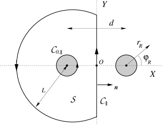
Figure 2: Configuration of two particles (top view) a lateral distance $d$ apart, trapped at an asymptotically flat interface. The left half ${\cal S}$ of the full interface is bounded by the particle–interface contact line ${\cal C}_{0}$ (generically noncircular), the oriented projection of which onto the $XY$–plane is ${\cal C}_{0,\parallel}$, and a contour ${\cal C}$, the oriented projection ${\cal C}_{\parallel}$ of which consists of a piece of the $Y$–axis and a circle of radius $L\to\infty$. The unit vector ${\bf n}$ is normal to the contour and directed towards the exterior of ${\cal S}$. The origin of the coordinate system is located at the midpoint $O$, while the coordinates $r_{R}$, $\varphi_{R}$ parametrize the plane with respect the center of the right particle.

The capillary deformation may give rise to an effective attraction between two identical particles trapped at the interface which could explain certain corresponding experimental observations. We compute this force using the electrostatic analogy derived above. The study of this issue will also clarify the general relationship between the force and the energy approaches as well as the respective advantages and disadvantages. We consider the equilibrium configuration of two particles at an asymptotically flat interface and fixed to be a distance $d$ apart (see Fig. 2). The total capillary force ${\bf F}_{\mathrm{total}}$ acting on the left half (which includes the piece ${\cal S}$ and the enclosed particle) is given by Eq. (2):

$${\bf F}_{\mathrm{total}}=\mbox{}-\oint_{{\cal C}}{\rm d}\ell\;({\bf e}_{t}\times{\bf e}_{n})\cdot\mathsf{T}.$$ (12)

If the particle separation $d$ is large enough, we can assume that the deformation of the interface at (but not necessarily inside) the contour ${\cal C}$ is small, so that the lateral force ${\bf F}_{\parallel}$ (= component of ${\bf F}_{\mathrm{total}}$ in the $XY$–plane = ${\bf F}_{\mathrm{total}}-({\bf F}_{\mathrm{total}}\cdot{\bf e}_{z}){\bf e}_{z}$) is (see Eq. (6c))

$${\bf F}_{\parallel}\approx\mbox{}-\oint_{{\cal C}_{\parallel}}{\rm d}\ell_{\parallel}\;{\bf n}\cdot\mathsf{T}_{\parallel}.$$ (13)

In the limit $L\to\infty$, the contribution from the circular part of ${\cal C}_{\parallel}$ vanishes and only the knowledge of the deformations at the straight midline part of ${\cal C}_{\parallel}$ is required, for which the electrostatic analogy will hold provided the interfacial deformations are small there. Thus, one can try to estimate the “electric potential” $u$ at the midline as $d\to\infty$ by a multipole expansion. The deformation field $u_{R}$ created by the right half plane behaves asymptotically like (see Appendix B)

$$u_{R}({\bf r}_{R})\sim\frac{Q_{0}}{2\pi\gamma}\ln\frac{\zeta}{r_{R}}+\frac{1}{2\pi\gamma}\sum_{s=1}^{\nu}\frac{Q_{s}\,{\rm e}^{-is\varphi_{R}}+Q_{s}^{*}\,{\rm e}^{is\varphi_{R}}}{2s(r_{R})^{s}}+\Delta u_{R}.$$ (14)

Here, ${\bf r}_{R}={\bf r}_{\parallel}-{\bf e}_{x}d/2$ is the position of a point relative to the center of the right particle (see Fig. 2), $\zeta$ is a fixed length determined by the distant boundary conditions, which set the zero point (undeformed interface) of the “electric potential” $u_{R}$, and $Q_{s}$ is given in terms of the $2^{s}$–pole of “capillary charge” associated with the particle and the surrounding interfacial deformation; if this is small everywhere, it is

$$Q_{s}=\int{\rm d}A_{R}\;(r_{R})^{s}\,{\rm e}^{is\varphi_{R}}\,\Pi_{\rm(single)}({\bf r}_{R})+\tilde{Q}_{s}^{\rm(single)},$$ (15)

with $\tilde{Q}_{s}^{\rm(single)}$ the corresponding charge associated to the particle (which is defined by the multipole expansion (see Eq. (50)) applied to the interfacial deformation at the contact line). The multipole expansion is based on the implicit assumption that the main source of the deformation field is concentrated at or near the particles. For that reason $Q_{s}$ is given by the “capillary charge” distribution for $d=\infty$, i.e., for the single–particle configuration. The asymptotically subdominant term $\Delta u_{R}$ in Eq. (14) accounts for the corrections to this assumption, i.e., “polarization” effects by the second particle and the fact that, even in the single–particle configuration, the pressure field $\Pi$ is expected to decay smoothly asymptotically far from the particles rather than dropping exactly to zero beyond some distance: if $\Pi(r_{\parallel}\to\infty)\sim r_{\parallel}^{-n}$ (actually $n=6$ in realistic models in the case of electric stresses Hurd (1985); Aveyard et al. (2000); Danov and Kralchevsky (2006); Domínguez et al. , and $n=8$ in the case of nematic stresses Oettel et al. (2008)), there is the bound $\nu<n-2$ (see the sum in Eq. (14) and Appendix B).

In general the leading term in the multipole expansion is determined by the “capillary monopole” $Q_{0}$. Thus asymptotically for $d\to\infty$, ${\bf F}_{\parallel}$ will be given by the “electric force” between two monopoles:

$${\bf F}_{\parallel}\approx\frac{Q_{0}^{2}}{2\pi\gamma d}{\bf e}_{x},$$ (16)

with the reversed sign as explained in the previous Section, so that it describes an attraction. Since $Q_{0}$ is given in terms of the net bulk force according to Eq. (10), the $1/d$-dependence only arises if there is an external field acting on the system. For example, Eq. (16) corresponds to the “flotation force” (at separations $d$ much smaller than the capillary length) for which ${\bf F}_{\rm bulk}$ is due to gravity. On the contrary, $Q_{0}$ will vanish if the system is mechanically isolated (so that any bulk forces acting on the particle are, according to the action–reaction principle, equal — but of oppositte sign — to any bulk forces acting on the interface and hence ${\bf F}_{\rm bulk}={\bf 0}$). This was the key point of a recent controversy as the force in Eq. (16) was advocated to explain certain experimental observations Nikolaides et al. (2002); Danov et al. (2004); Smalyukh et al. (2004) while missing that mechanical isolation (as purported in the experiments) rules out this force Megens and Aizenberg (2003); Foret and Würger (2004); Oettel et al. (2005a, 2006, 2008).

If $Q_{0}=0$, the capillary force is determined by higher-order terms in the multipole expansion (14). Mechanical isolation implies the vanishing of the net bulk force and torque, i.e., “capillary monopole” and “capillary dipole” (see Eqs. (10, 11)). Thus in general, ${\bf F}_{\parallel}$ will take the form of a force between quadrupoles, i.e., it is anisotropic and scales as

$$|{\bf F}_{\parallel}|\propto\frac{|Q_{2}|^{2}}{d^{5}}.$$ (17)

An experimental realization of this case corresponds to nonspherical inert particles, so that $\Pi\equiv 0$ and the interfacial deformation is solely due to an undulated contact line (for a recent corresponding experimental study see Ref. Loudet et al., 2006). Concerning the possibility to relate corresponding experimental observations and theoretical descriptions we point out the difficulty that $Q_{2}$ and higher “capillary poles” are known only in terms of the deformation field $u$, in contrast to $Q_{0}$ and $Q_{1}$, which are given by the directly measurable and independently accessible quantities “bulk force” and “bulk torque”, respectively.

Another experimentally relevant situation of mechanical isolation corresponds to the case that the “capillary charges” $Q_{s}$ of all orders $s\geq 0$ vanish. For example, for an electrically charged, spherical particle in mechanical isolation one has $Q_{0}=0$ and $Q_{1}=0$ by mechanical isolation, and by symmetry a rotationally invariant interfacial deformation in the single–particle configuration, giving $Q_{s}=0$ also for any $s\geq 2$. In this case Eq. (14) reduces to the correction $\Delta u_{R}$ and the computation of ${\bf F}_{\parallel}$ requires a specific model for $\Pi({\bf r}_{\parallel})$ and a detailed calculation. In view of our present purposes, we qualitatively derive only a bound on how rapidly ${\bf F}_{\parallel}$ decays as function of the separation $d$.

The correction $\Delta u_{R}(r_{R}\to\infty)$ has a contribution $\sim(r_{R})^{2-n}$ already in the single–particle configuration because the rotationally symmetric “charge density” $\Pi(r_{R}\to\infty)\sim(r_{R})^{-n}$ does not have a compact support (see Appendix B). This provides a contribution to the capillary force ${\bf F}_{\parallel}$ which is equal to the force between the “capillary charges” at each side of but near the midline because the presence of the second particle breaks the rotational symmetry. This force can be estimated to decay like $d^{-1+2(2-n)}$ because the net “capillary charge” in the region farther than a distance $d$ from one particle is $\sim\int_{r_{\parallel}>d}dA_{\parallel}\;\Pi\sim d^{2-n}$ and the force between charges decays $\sim d^{\mbox{}-1}$.

Additionally, $\Delta u_{R}$ has genuine two–particle contributions “induced” by the second particle which can be modeled by means of “induced capillary charges” $Q_{s}(d)$ depending on the particle separation. Generically the dominant term will be a “capillary dipole” giving rise to a correspondingly dipole-dipole force $\sim|Q_{1}(d)|^{2}/d^{3}$, where the “induced dipole” $Q_{1}(d)$ must decay at least like the inducing field. This is caused by various reasons. If $Q_{1}(d)$ arises by a violation of the boundary conditions at the contact line, one has $Q_{1}(d)={\cal O}(\Delta u_{R}(d))\sim d^{2-n}$, and the force decays by a factor $1/d^{2}$ faster than the contribution discussed above concerning the violation of rotational symmetry. But there can also be deviations from the linear superposition of the pressure on the interface. This occurs, e.g., if the interfacial deformation is due to electric fields emanating from the particles, so that $\Pi\propto E^{2}$ and $\Pi({\bf r}_{\parallel})-[\Pi_{\rm(single)}({\bf r}_{R})+\Pi_{\rm(single)}({\bf r}_{L})]\propto E_{\rm(single)}({\bf r}_{R})\,E_{\rm(single)}({\bf r}_{L})$. In this case one has $Q_{1}(d)={\cal O}(E_{\rm(single)}(d))\sim d^{-n/2}$. Thus we can conclude that the lateral force must decay as function of separation asymptotically at least as

$$F_{\parallel}={\cal O}(d^{\mbox{}-\min{(2n-3,n+3)}}),$$ (18)

depending on the value of $n$. In any case this force decays more rapidly than the expression given by Eq. (16).

It is instructive to compare $F_{\parallel}$ with the force obtained within the energy approach. The latter consists of finding the parametric dependence on $d$ of the free energy for the two–particle configuration,

$$V_{\mathrm{men}}=\int_{{\cal S}_{\parallel}}{\rm d}A_{\parallel}\;\left[\,\frac{\gamma}{2}\,|\nabla_{\parallel}u|^{2}-\Pi\,u\right]+V_{\mathrm{part}},$$ (19)

where the integral is the contribution by the interface and $V_{\mathrm{part}}$ collects the direct contribution by the particles Oettel et al. (2005a); Domínguez et al. (2007a). (Within the electrostatic analogy, the effect of $V_{\mathrm{part}}$ would be replaced by appropriate boundary conditions on the “potential” $u$ at the interface–particle contact lines.) $V_{\mathrm{men}}(d)$ plays the role of a “potential of mean force” for the particle–particle interaction, giving rise to a corresponding “mean force”

$$F_{\mathrm{men}}(d)=\mbox{}-V^{\prime}_{\mathrm{men}}(d)$$ (20)

upon integrating out the capillary degrees of freedom within thermal equilibrium. One should keep in mind that this approach captures only the mean–fieldlike contribution to the mean force. The capillary wavelike fluctuations of the interface around the mean meniscus profile generates additional, Casimir–like contributions to the force Lehle et al. (2006); Lehle and Oettel (2007), which we do not consider in the following.

One can distinguish two cases. First, if there are “permanent capillary charges” ($Q_{0}\neq 0$ if the system is not mechanically isolated, or $Q_{s}\neq 0$ for some $s\geq 2$ for mechanical isolation, as discussed above), $F_{\parallel}$ coincides with $F_{\mathrm{men}}$; see, e.g., Refs. Nicolson, 1949; Chan et al., 1981; Oettel et al., 2005a for a derivation of Eq. (16) or Refs. Stamou et al., 2000; Kralchevsky et al., 2001; Fournier and Galatola, 2002; van Nierop et al., 2005 for obtaining Eq. (17) in the context of the energy approach with the simplifying assumption that the interface deformation is small everywhere. The reasoning presented here extends, however, this result also to the case that the deformation around the particles is not small, requiring this only near the midline between the particles, i.e., asymptotically for $d\to\infty$. Furthermore, the electrostatic analogy shows immediately that the capillary forces $F_{\parallel}$ are asymptotically pairwise additive in a configuration with more than two particles provided they possess a nonvanishing “permanent capillary pole”.

The second case corresponds to the absence of “permanent capillary charges” as described above. This has been thoroughly investigated in Refs. Oettel et al., 2005b; Würger and Foret, 2005; Domínguez et al., 2007a within the energy approach, and has led to $F_{\mathrm{men}}(d)\sim d^{-1-n/2}$, which does not agree with any of the possible asymptotic decays indicated in Eq. (18). In order to understand this discrepancy, we recall that by definition (Eq. (13)) ${\bf F}_{\parallel}$ represents the net force acting on the subsystem formed by the particle and the piece of interface enclosed by the contour indicated in Fig. 2. The work done by this force upon an infinitesimal virtual displacement $\delta d$ is not related in any simple manner to the change $\delta V_{\mathrm{men}}$, which according to the definition in Eq. (19) will involve the work done by local forces during the rearrangement of the “capillary charges” inside the subsystem, so that in general $F_{\parallel}\neq F_{\mathrm{men}}$.

In conclusion one has $F_{\parallel}=F_{\mathrm{men}}$ if the $d$–dependence of $V_{\mathrm{men}}(d)$ is dominated asymptotically by a multipole expansion, i.e., the whole subsystem can be replaced by a set of point “capillary poles”: the degrees of freedom related to the internal structure are irrelevant and only the separation $d$ and the orientation of the “capillary poles” matter. This is related to the validity of the “superposition approximation”Nicolson (1949) usually employed in the energy approach, which consists of approximating the deformation field $u$ by the sum of the deformation fields induced by each particle in the single–particle configuration. In Ref. Domínguez et al., 2007a it is shown that this approximation is valid if the system is not mechanically isolated because in that case, asymptotically for $d\to\infty$, the interface–mediated effect of one particle on the other amounts to shift it — together with its surrounding interface — vertically as a whole, i.e., without probing or affecting the “internal structure” of the subsystem “particle plus surrounding interface”.

Finally, it is clear that both $F_{\parallel}$, defined in Eq. (13), and $F_{\mathrm{men}}$, defined in Eq. (20), include a contribution from $\Pi$ and thus differ from the force acting only on the colloidal particle (which would be the integral in Eq. (13) extended only along the particle–interface contact line). If one is interested in physical situations in thermal equilibrium, $F_{\mathrm{men}}$ does represent the effective force between the particles, i.e., once the capillary degrees of freedom have been integrated out. In dynamical situations out of equilibrium, completely new considerations have to be made concerning, e.g., whether the capillary degrees of freedom can be assumed to have relaxed towards thermal equilibrium in the dynamical time scale of interest. But this discussion lies beyond the scope of the present analysis.

IV Nonplanar reference interface

In the following we shall discuss some applications of Eq. (1) for particles trapped at an interface which in its unperturbed state is curved. In Subsec. IV.1 we shall first consider the interfacial deformation induced by a single charged particle on an otherwise spherical droplet. This configuration is particularly relevant for the experiment described in Ref. Nikolaides et al., 2002. As explained in the previous section, mechanical isolation rules out a monopolarlike (i.e., logarithmic) deformation if the unperturbed interface is flat. Since there has been recently a controversy whether this conclusion is altered by the curvature of the droplet, we shall present a thorough analysis for such systems. In Subsec. IV.2 the application of the electrostatic analogy to a generally curved interface is illustrated.

IV.1 Particle on a spherical droplet

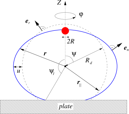
Figure 3: Charged colloidal particle (radius $R$) at the interface of a droplet residing on a plate. Positions on the interface are parametrized by the polar angle $\psi$ and the revolution angle $\varphi$. Without the colloidal particle and neglecting gravity the droplet has spherical shape with radius $R_{\mathrm{d}}$ and normal vector ${\bf e}_{r}$. ${\bf r}_{\parallel}=R_{\mathrm{d}}{\bf e}_{r}(\psi,\varphi)$ is a point at the unperturbed, spherical interface (dashed line) whereas ${\bf r}={\bf r}_{\parallel}+u(\psi,\varphi){\bf e}_{r}$ is a point at the perturbed, nonspherical interface (full line). The perturbed interface intersects the plate for $\psi=\psi_{1}$.

We consider a charged spherical particle of radius $R$ trapped at the interface of a droplet which resides on a plate (Fig. 3). This configuration models the experiment described in Ref. Nikolaides et al., 2002 in the absence of gravity. Our goal is to compute the deformation of the droplet far from the particle. Compared with the energy approach, the force approach has two advantages: (i) The result is more general because we have to assume only that the deformation is small far from the particle; the usual linear approximation is not required to hold also near the particle. (ii) The boundary condition “mechanical equilibrium of the particle” is incorporated easily irrespective of the details how the particle is attached to the interface. It will turn out that the implementation of this condition has been the source of mistakes in the literature.

We apply Eq. (1) to the piece ${\cal S}(\Psi)$ of the curved interface bounded on one side by the particle–interface contact line ${\cal C}_{0}$ and on the other side by a circle given by the constant latitude $\Psi$, ${\cal C}(\Psi):=\{\psi=\Psi\leq\psi_{1}\}$, so that $\partial{\cal S}={\cal C}_{0}\cup{\cal C}(\Psi)$, and we assume that the particle is located at the apex opposite to the plate (Fig. 3). The unperturbed state corresponds to an uncharged particle which does not exert a force on the interface, so that the equilibrium shape of the interface is spherical. In the presence of electric charges, the interface will deform. If the particle stays at the upper apex, also the deformed interface exhibits axial symmetry. We rewrite Eq. (1) in three steps.

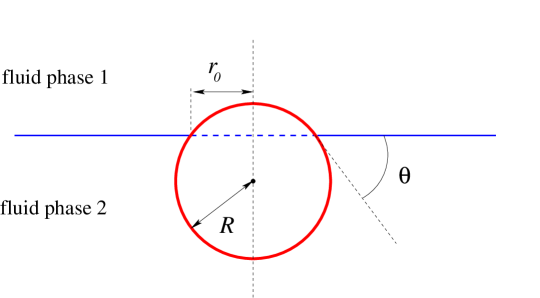
Figure 4: Side view of a single electrically neutral and spherical particle at a planar fluid interface in equilibrium. The radius $r_{0}=R\sin\theta$ of the circular contact line follows from the equilibrium contact angle $\theta$. If the interface was that of a large droplet (radius $R_{\mathrm{d}}\gg R$, see Fig. 3), this expression would exhibit correction terms of order $R/R_{\mathrm{d}}$. In the same manner, the presence of charges would deform the interface and introduce corrections which in first order are proportional to the deformation.

(i) The pressure splits into

$$\Pi({\bf r})=\Delta p+\Pi_{\mathrm{el}}({\bf r}),\qquad\Delta p=\frac{2\gamma}{R_{\mathrm{d}}}\left(1-\mu/2\right).$$ (21)

Here, $R_{\mathrm{d}}$ is the radius of the unperturbed, spherical droplet, and $2\gamma/R_{\mathrm{d}}$ is the pressure jump across the interface in the unperturbed state. The dimensionless constant $\mu$ accounts for the change in hydrostatic pressure due to enforcing the condition of constant droplet volume in the presence of interface deformations. $\Pi_{\mathrm{el}}({\bf r})$ is the pressure field created by the electric field emanating from the particle which includes electric stresses and an osmotic pressure due to a possible discontinuity of the ion concentrations at the interface (see, e.g., Refs. Shestakov et al., 2002; Würger, 2006a); this pressure field follows from solving the corresponding electrostatic problem. We write

$$\int_{{\cal S}}{\rm d}A\;{\bf e}_{n}\Pi_{\mathrm{el}}=2\pi\gamma r_{0}\,\boldsymbol{\varepsilon}_{\Pi}-\int_{\cal S_{\mathrm{men}}\backslash\cal S}\!\!\!\!\!\!{\rm d}A\;{\bf e}_{n}\Pi_{\mathrm{el}},$$ (22)

where we have introduced the dimensionless electric force acting on the whole interface ${\cal S}_{\mathrm{men}}$ (which at the apex has a hole carved out),

$$\boldsymbol{\varepsilon}_{\Pi}:=\frac{1}{2\pi\gamma r_{0}}\int_{\cal S_{\mathrm{men}}}\!\!\!\!\!\!{\rm d}A\;{\bf e}_{n}\Pi_{\mathrm{el}}.$$ (23)

Here $r_{0}=R\sin\theta$, where $\theta$ is the equilibrium contact angle between the fluid phases and the particle; $r_{0}$ is actually the radius of the circular contact line of the uncharged particle at a planar interface (see Fig. 4).

(ii) Since the particle is in mechanical equilibrium, the contact line force must be balanced by the hydrostatic force ${\bf F}_{\Delta p}$ and the electric force ${\bf F}_{\mathrm{el}}$ acting on the particle, as well as by any other force ${\bf F}_{\mathrm{ext}}$ of external origin (e.g., an optical tweezer pushing or pulling the particle):

$$\gamma\oint_{{\cal C}_{0}}{\rm d}\ell\;{\bf e}_{t}\times{\bf e}_{n}={\bf F}_{\Delta p}-2\pi\gamma r_{0}(\boldsymbol{\varepsilon}_{\mathrm{el}}+\boldsymbol{\varepsilon}_{\mathrm{ext}}),$$ (24)

where we have introduced the dimensionless electric and external forces acting on the particle:

$$\boldsymbol{\varepsilon}_{\mathrm{el}}:=-\frac{{\bf F}_{\mathrm{el}}}{2\pi\gamma r_{0}},\quad\boldsymbol{\varepsilon}_{\mathrm{ext}}:=-\frac{{\bf F}_{\mathrm{ext}}}{2\pi\gamma r_{0}}.$$ (25)

(iii) Finally, the following identity is a consequence of elementary considerations of hydrostatics because $\Delta p$ in Eq. (21) is spatially constant:

$$\int_{{\cal S}(\Psi)}{\rm d}A\;{\bf e}_{n}\Delta p+{\bf F}_{\Delta p}={\bf e}_{z}A_{z}(\Psi)\Delta p,$$ (26)

where $A_{z}(\Psi)$ is the circular area in the $XY$ plane bounded by the circle ${\cal C}(\Psi)$.

Thus Eq. (1) can be rewritten as

$$\gamma\oint_{{\cal C}(\Psi)}{\rm d}\ell\;{\bf e}_{t}\times{\bf e}_{n}=2\pi\gamma r_{0}(\boldsymbol{\varepsilon}_{\mathrm{ext}}+\boldsymbol{\varepsilon}_{\mathrm{el}}-\boldsymbol{\varepsilon}_{\Pi})-{\bf e}_{z}A_{z}(\Psi)\Delta p+\int_{\cal S_{\mathrm{men}}\backslash\cal S}\!\!\!\!\!\!{\rm d}A\;{\bf e}_{n}\Pi_{\mathrm{el}}.$$ (27)

With the notation introduced in Fig. 3, one has (as in Sec. II, the subscript _∥ denotes quantities evaluated at and operators acting in the undeformed spherical interface, i.e., in tangent planes of the undeformed interface):

$${\bf e}_{n}\,{\rm d}A = \left(\frac{\partial{\bf r}}{\partial\psi}\times\frac{\partial{\bf r}}{\partial\varphi}\right){\rm d}\psi{\rm d}\varphi=\left(1+\frac{u}{R_{\mathrm{d}}}\right)\left[\left(1+\frac{u}{R_{\mathrm{d}}}\right){\bf e}_{r}-\nabla_{\parallel}u\right]{\rm d}A_{\parallel},$$ (28a)

$${\bf e}_{t}\,{\rm d}\ell = ({\rm d}\boldsymbol{\ell}_{\parallel}\cdot\nabla_{\parallel}){\bf r}=\left[1+\frac{u}{R_{\mathrm{d}}}\right]{\rm d}\boldsymbol{\ell}_{\parallel}+{\bf e}_{r}({\rm d}\boldsymbol{\ell}_{\parallel}\cdot\nabla_{\parallel}u),$$ (28b)

where ${\rm d}\boldsymbol{\ell}_{\parallel}=R_{\mathrm{d}}({\bf e}_{\psi}{\rm d}\psi+{\bf e}_{\varphi}\sin\psi\,{\rm d}\varphi)$, ${\rm d}A_{\parallel}=R_{\mathrm{d}}^{2}\sin\psi\,{\rm d}\psi{\rm d}\varphi$, and

$$\nabla_{\parallel}=\frac{{\bf e}_{\psi}}{R_{\mathrm{d}}}\frac{\partial}{\partial\psi}+\frac{{\bf e}_{\varphi}}{R_{\mathrm{d}}\sin\psi}\frac{\partial}{\partial\varphi}.$$ (29)

With this notation, $A_{z}(\Psi)=\pi[R_{\mathrm{d}}+u(\Psi)]^{2}\sin^{2}\Psi$. Equation (27) can be simplified under the assumption that deviations of the actual droplet shape from the spherical one of radius $R_{\mathrm{d}}$ are small in the distant region $R/R_{\mathrm{d}}\ll\Psi\leq\psi<\psi_{1}$, so that the linearized approximation of the deformation is valid and terms quadratic in the quantities $u$, $\mu$, and $\Pi_{\mathrm{el}}$ (which vanish in the unperturbed state) can be omitted Oettel et al. (2005a). We emphasize that this condition does not exclude large deviations within the piece ${\cal S}(\Psi)$, in particular near the particle. Due to rotational symmetry, the vectorial Eq. (27) is independent of the angle $\varphi$ and involves only vectors parallel to ${\bf e}_{z}$. One obtains the following ordinary differential equation for the function $u(\Psi)$:

$$\sin\Psi\cos\Psi\frac{\partial u}{\partial\Psi}=r_{0}\,{\bf e}_{z}\cdot(\boldsymbol{\varepsilon}_{\mathrm{ext}}+\boldsymbol{\varepsilon}_{\mathrm{el}}-\boldsymbol{\varepsilon}_{\Pi})+\left(\frac{1}{2}\mu R_{\mathrm{d}}-u\right)\sin^{2}\Psi+\frac{R_{\mathrm{d}}^{2}}{\gamma}\int_{\Psi}^{\psi_{1}}\!\!\!{\rm d}\psi\;\sin\psi\cos\psi\;\Pi_{\mathrm{el}}(\psi).$$ (30)

This expression is actually the first integral of the Young–Laplace equation (Eq. (B7) in Ref. Oettel et al., 2005a) incorporating the boundary condition at the contact line. In terms of the functions $P(\psi):=\cos\psi$, $Q(\psi):=1+\cos\psi\,\ln\tan(\psi/2)$ and

$$S(\psi):=-\frac{R_{\mathrm{d}}^{2}}{\gamma}\int_{\psi}^{\psi_{1}}\!\!\!{\rm d}s\,\sin s\;\Pi_{\mathrm{el}}(s)[P(\psi)Q(s)-P(s)Q(\psi)],$$ (31)

the general solution is

$$u(\psi)=AP(\psi)+r_{0}\,{\bf e}_{z}\cdot(\boldsymbol{\varepsilon}_{\mathrm{ext}}+\boldsymbol{\varepsilon}_{\mathrm{el}}-\boldsymbol{\varepsilon}_{\Pi})Q(\psi)+\frac{1}{2}\mu R_{\mathrm{d}}+S(\psi),$$ (32)

where $\mu$ and the integration constant $A$ can be determined by the boundary condition at the plate, i.e., $\psi=\psi_{1}$, and the incompressibility condition of the droplet Oettel et al. (2005a). In the limit $R_{\mathrm{d}}\to\infty$ at fixed $r=R_{\mathrm{d}}\psi$, one recovers the results of an unperturbed, planar interface Domínguez et al. (2005). We are particularly interested in the deformation given by Eq. (32) in the intermediate range $R/R_{\mathrm{d}}\ll\psi\ll 1$, i.e., far from the particle and from the plate. In this range, $P(\psi)\sim 1$, $Q(\psi)\sim\ln\psi+\mbox{}$const., whereas $\Pi_{\mathrm{el}}(\psi)$ will decay in general as $\psi^{-n}$, implying $S(\psi)\sim\psi^{2-n}$ if $n>2$. Thus due to the behavior of $Q(\psi)$ there may be a logarithmically varying asymptotic deformation with the amplitude given by $r_{0}\,{\bf e}_{z}\cdot(\boldsymbol{\varepsilon}_{\mathrm{ext}}+\boldsymbol{\varepsilon}_{\mathrm{el}}-\boldsymbol{\varepsilon}_{\Pi})$.

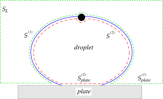
Figure 5: The surface ${\cal S}^{(1)}$ (${\cal S}^{(2)}$) runs along the fluid interface (full line) and the particle (dot) such that it lies in the fluid phase exterior (interior) to the droplet. The surface ${\cal S}_{plate}^{(1)}$ (${\cal S}_{plate}^{(2)}$) is that part of the plate surface which is in contact with the fluid phase exterior (interior) to the droplet. The surface ${\cal S}_{L}$ encloses the whole system “particle + fluid phases” at a macroscopic distance $L\to\infty$ from the droplet. The surfaces are oriented towards the exterior of the corresponding fluid volume which they enclose.

We now consider the situation that there is no external field acting on the system. In this case $\boldsymbol{\varepsilon}_{\mathrm{ext}}={\bf 0}$ and the electric forces $\boldsymbol{\varepsilon}_{\mathrm{el}}$ and $\boldsymbol{\varepsilon}_{\Pi}$ are only due to the charge of the particle. The value of $\boldsymbol{\varepsilon}_{\mathrm{el}}-\boldsymbol{\varepsilon}_{\Pi}$ can be obtained by adapting the reasoning of Ref. Oettel et al., 2005a to the droplet geometry. The stress tensor in the fluid phase exterior to the droplet is given as $\mbox{}-p_{1}\mathsf{1}+\mathsf{T}_{\rm el}^{(1)}$, where $p_{1}\mathsf{1}$ is the homogeneous, isotropic stress tensor far from the droplet and $\mathsf{T}_{\rm el}^{(1)}$ is Maxwell’s stress tensor due to the electric field (modified to include the possible osmotic pressure by mobile charges, see, e.g., Ref. Shestakov et al., 2002). In the same manner, $\mbox{}-(p_{1}+\Delta p)\mathsf{1}+\mathsf{T}_{\rm el}^{(2)}$ is the stress tensor in the interior of the droplet, where $\Delta p$ is given by Eq. (21). With the notations introduced in Fig. 5, the following equations hold:

$$\int_{{\cal S}_{plate}^{(1)}\cup{\cal S}_{L}\cup{\cal S}^{(1)}}{\rm d}{\bf A}\cdot\mathsf{T}_{\rm el}^{(1)}={\bf 0},$$ (33a)

$$\int_{{\cal S}_{plate}^{(2)}\cup{\cal S}^{(2)}}{\rm d}{\bf A}\cdot\mathsf{T}_{\rm el}^{(2)}={\bf 0},$$ (33b)

which express that the net force on the exterior fluid phase and on the interior one, respectively, vanishes in equilibrium. (The contribution to the integrals from the constant isotropic pressures $p_{1}$ and $p_{1}+\Delta p$ is zero.) On the other hand, by definition one has

$$2\pi\gamma r_{0}(\boldsymbol{\varepsilon}_{\Pi}-\boldsymbol{\varepsilon}_{\mathrm{el}})=\mbox{}-\int_{{\cal S}^{(1)}}{\rm d}{\bf A}\cdot\mathsf{T}_{\rm el}^{(1)}-\int_{{\cal S}^{(2)}}{\rm d}{\bf A}\cdot\mathsf{T}_{\rm el}^{(2)}.$$ (34)

Combining this with Eqs. (33) leads to

$$\boldsymbol{\varepsilon}_{\Pi}-\boldsymbol{\varepsilon}_{\mathrm{el}}=\frac{1}{2\pi\gamma r_{0}}\left[\int_{{\cal S}_{plate}^{(1)}}{\rm d}{\bf A}\cdot\mathsf{T}_{\rm el}^{(1)}+\int_{{\cal S}_{plate}^{(2)}}{\rm d}{\bf A}\cdot\mathsf{T}_{\rm el}^{(2)}\right],$$ (35)

where we have taken into account that the contribution of $\mathsf{T}_{\rm el}^{(1)}$ over the surface ${\cal S}_{L}$ vanishes in the limit $L\to\infty$ because the electric field decays to zero far away from the droplet (i.e., we do not consider the possibility that there are external electric fields). That is, $\mbox{}-(\boldsymbol{\varepsilon}_{\Pi}-\boldsymbol{\varepsilon}_{\mathrm{el}})$ is actually the (dimensionless) electric force acting on the plate. The calculation of this integral requires to solve the corresponding electrostatic problem. However, on dimensional grounds one can obtain the estimate $|\boldsymbol{\varepsilon}_{\Pi}-\boldsymbol{\varepsilon}_{\mathrm{el}}|\sim|\boldsymbol{\varepsilon}_{\Pi}|(r_{0}/R_{\mathrm{d}})^{n-2}$. For an asymptotically planar interface, the logarithmically varying deformation due to nonzero values of $|\boldsymbol{\varepsilon}_{\Pi}-\boldsymbol{\varepsilon}_{\mathrm{el}}|$ leads to a long–ranged effective attraction (see Sec. III), which is the reason that this mechanism has been invoked to be responsible for the apparent attraction reported in Ref. Nikolaides et al., 2002. If this was the explanation, the measurements in this experiment would imply a value Oettel et al. (2005a) $|\boldsymbol{\varepsilon}_{\Pi}-\boldsymbol{\varepsilon}_{\mathrm{el}}|\sim 10^{-3}$. On the other hand, the theoretical estimate yields $|\boldsymbol{\varepsilon}_{\Pi}-\boldsymbol{\varepsilon}_{\mathrm{el}}|\sim 10^{-6}|\boldsymbol{\varepsilon}_{\Pi}|$ with $n=6$, so that the experimental results would require $|\boldsymbol{\varepsilon}_{\Pi}|\sim 10^{3}$. This large value is unlikely for realistic surface charge densities Oettel et al. (2005a, b).

This result corrects the suggestion made in Ref. Oettel et al., 2005a that $|\boldsymbol{\varepsilon}_{\Pi}-\boldsymbol{\varepsilon}_{\mathrm{el}}|\sim(r_{0}/R_{\mathrm{d}})^{2}$, inferred from a not applicable force balance condition. Indeed, if the deformation is small also at the contact line, the condition “mechanical equilibrium of the particle” can be derived from Eq. (30) and with an expansion in terms of $\psi_{0}=r_{0}/R_{\mathrm{d}}\ll 1$ leads to

$$\left.\frac{{\rm d}u}{{\rm d}\psi}\right|_{\psi=\psi_{0}}\approx R_{\mathrm{d}}\,{\bf e}_{z}\cdot(\boldsymbol{\varepsilon}_{\mathrm{ext}}+\boldsymbol{\varepsilon}_{\mathrm{el}})+\psi_{0}\left[\frac{1}{2}\mu R_{\mathrm{d}}-u(\psi_{0})\right].$$ (36)

The second term, which is subdominant in the limit $R_{\mathrm{d}}\to\infty$, is missing in Eq. (B8) of Ref. Oettel et al., 2005a. We have cross-checked this corrected expression by deriving it also within the energy approach employed in Ref. Oettel et al., 2005a, which turns out to be algebraically much more cumbersome.

In conclusion, there persists a logarithmically varying deformation with an amplitude which is very small in the limit $R_{\mathrm{d}}\to\infty$; this is actually a finite–size effect intrinsic to the geometry of the set-up and absent for an unbounded flat interface. However, it has the same physical origin as any logarithmically varying deformation of a flat interface, namely that the system “particle + fluid interface” cannot be mechanically isolated in the configuration of a droplet residing on a solid plate. In the absence of the plate one has $\boldsymbol{\varepsilon}_{\Pi}-\boldsymbol{\varepsilon}_{\mathrm{el}}={\bf 0}$ due to Eq. (35) because ${\cal S}_{plate}^{(1)}$ and ${\cal S}_{plate}^{(2)}$ are not there and the logarithmic dependence in the range $\psi\ll 1$ disappears. This conclusion corrects a recent claim of the opposite in Ref. Würger, 2006b; the relevant errors of this work are pinpointed in Ref. Domínguez et al., 2007b, in particular the implementation of the boundary condition “mechanical equilibrium of the particle”. (Reference Domínguez et al., 2007b represents incidentally, within the energy approach, a further confirmation of our conclusion above.) To facilitate the comparison of our calculations with Ref. Würger, 2006b we make two remarks: (i) The reasoning and results are independent of the precise functional form of the electric pressure $\Pi_{\mathrm{el}}({\bf r})$; the considerations in Ref. Würger, 2006b in this respect are thus irrelevant. (ii) As a boundary condition for fixing the droplet Ref. Würger, 2006b employs, instead of a plate at $\psi=\psi_{1}$ as used here, a fictional pressure field $\Pi_{\mathrm{com}}(\psi)\propto\cos\psi$ constraining the center of mass of the droplet Morse and Witten (1993). One can easily check that our general solution (Eq. (32)) includes this special case, as the contribution of $\Pi_{\mathrm{com}}(\psi)$ in Eq. (32) eliminates the singularity of $Q(\psi)$ at $\psi=\pi$ and the solution reduces to the corresponding expression in Ref. Würger, 2006b. Thus none of these two issues affects the conclusion concerning the logarithmic dependence.

IV.2 Particle on a generally curved interface

If the particle is trapped at a generally curved interface (reference interface), the electrostatic analogy can still be exploited provided there is a clear separation of length scales between the typical radius of curvature $R_{\mathrm{d}}$ of the reference interface and the size of the region around the particle where the interfacial deformations are appreciable, say, roughly a few times the particle size $R$. Then, at distances from the particle smaller than $R_{\mathrm{d}}$ one can exploit the electrostatic analogy in order to study the small deviations of the interface from a reference plane tangent to the reference interface at some fixed point near the particle.

The deviations from the reference plane are given by the displacement field $u({\bf r}_{\parallel})=u_{\rm ref}({\bf r}_{\parallel})+\delta u({\bf r}_{\parallel})$, where $u_{\rm ref}({\bf r}_{\parallel})$ is the deformation of the reference interface and $\delta u({\bf r}_{\parallel})$ is the additional deformation brought about by the presence of the particle. Correspondingly, the pressure field can be written as $\Pi=\Pi_{\rm ref}+\delta\Pi$. If $\ell$ is a distance from the particle beyond which the linearized theory holds (i.e., the deformation near the particle need not be small), then in the annulus $\ell<r_{\parallel}<R_{\mathrm{d}}$ (with a clear separation $\ell\ll R_{\mathrm{d}}$ so that the following dependence can be observed) the solution to the field equation can be written as

$$\delta u({\bf r}_{\parallel}) = B_{0}\ln\frac{\zeta}{r_{\parallel}}+\sum_{s=1}^{\infty}\frac{1}{2s}\left\{\frac{B_{s}\,{\rm e}^{-is\varphi}+B_{s}^{*}\,{\rm e}^{is\varphi}}{r_{\parallel}^{s}}+r_{\parallel}^{s}[A_{s}\,{\rm e}^{is\varphi}+A_{s}^{*}\,{\rm e}^{-is\varphi}]\right\}$$ (37)

$$+\frac{1}{2\pi\gamma}\int_{\ell<r^{\prime}<R_{\mathrm{d}}}dA^{\prime}_{\parallel}\;\delta\Pi({\bf r}_{\parallel}^{\prime})\ln\frac{\zeta}{|{\bf r}_{\parallel}-{\bf r}_{\parallel}^{\prime}|}.$$

The constants $A_{s}$ and $B_{s}$ are determined by the boundary conditions at $r=\ell$ and $r=R_{\mathrm{d}}$ and account for “virtual capillary charges” outside the annulus. In particular, we have already seen that $2\pi\gamma B_{0}$ is the net bulk force on the region $r<\ell$ in the direction normal to the reference plane (and in addition to the net force in the reference state $u_{\rm ref}({\bf r}_{\parallel})$).

Two new issues arise which we have not considered so far: there is an “external boundary” given by the upper bound $r_{\parallel}=R_{\mathrm{d}}$ and there is a nonvanishing reference deformation $u_{\rm ref}({\bf r}_{\parallel})$. The first issue is not exclusive for a curved reference interface and emerges if the interfacial pressure $\Pi({\bf r}_{\parallel})$ does not decay sufficiently fast with the separation from the particle, so that in principle one cannot carry out the limit $R_{\mathrm{d}}\to\infty$. An example has been studied in full detail in the previous subsection, where $\delta\Pi$ includes a term $-\mu\gamma/R_{\mathrm{d}}$ (see Eq. (21)) generated by a nonlocal constraint (i.e., constant volume of the droplet). In general, the relevance of the boundary conditions at $r_{\parallel}=R_{\mathrm{d}}$ introduces a nonlocal ingredient preventing general statements based just on the electrostatic analogy localized around the particle.

The second issue implies an “external electric field”, $-\nabla_{\parallel}u_{\rm ref}$, giving rise to a new phenomenology. To illustrate this point, we consider a reference minimal surface, $\nabla_{\parallel}^{2}u_{\rm ref}=0$ (so that $\Pi_{\rm ref}\equiv 0$), containing a mechanically isolated nonspherical inert particle (so that $\delta\Pi\equiv 0$) with extension $R$ much smaller than the typical curvature radius $R_{\mathrm{d}}$ of the reference interface. As we have seen, $Q_{0}=Q_{1}=0$ (i.e., no bulk force normal to the reference plane and no torque in that plane), but $Q_{2}\neq 0$, so that the particle will experience a force and a torque which are given, to leading order in the small ratio $R/R_{\mathrm{d}}$, by the coupling of this quadrupole with the “external field” $u_{\rm ref}$. According to Eq. (52), the real-valued quadrupole is characterized by the following 2nd rank tensor:

$$\hat{Q}_{2}=q_{2}\left[({\bf e}_{x}{\bf e}_{x}-{\bf e}_{y}{\bf e}_{y})\cos 2\theta+({\bf e}_{x}{\bf e}_{y}+{\bf e}_{y}{\bf e}_{x})\sin 2\theta\right],$$ (38)

where $q_{2}>0$ is the amplitude and $\theta$ is the angle which the principal axes of the quadrupole form with the coordinate axes. The origin of coordinates, ${\bf r}_{\parallel}={\bf 0}$, is the contact point of the reference tangent plane with the interface and must be taken at some point in or close to the particle, e.g., its center of mass. In these circumstances, the electrostatic analogy provides the force and the torque, respectively, as

$${\bf F}=\frac{1}{2}\nabla_{\parallel}\left[\hat{Q}_{2}:\nabla_{\parallel}\nabla_{\parallel}u_{\rm ref}\right]_{{\bf r}_{\parallel}={\bf 0}},$$ (39)

$${\bf M}=-\nabla_{\parallel}\times\left[\hat{Q}_{2}\cdot\nabla_{\parallel}u_{\rm ref}\right]_{{\bf r}_{\parallel}={\bf 0}},$$ (40)

after reversing the sign with respect to the electrostatic expressions, as discussed above. The most general form of the traceless Hessian matrix of the reference interface is given by

$$\nabla_{\parallel}\nabla_{\parallel}u_{\rm ref}({\bf r})=\frac{1}{R_{\mathrm{d}}({\bf r})}\left[({\bf e}_{x}{\bf e}_{x}-{\bf e}_{y}{\bf e}_{y})\cos 2\phi({\bf r})+({\bf e}_{x}{\bf e}_{y}+{\bf e}_{y}{\bf e}_{x})\sin 2\phi({\bf r})\right],$$ (41)

where $R_{d}({\bf r})>0$ is the absolute value of the radius of curvature and $\phi({\bf r})$ is the angle between the principal directions and the coordinate axes. Without loss of generality one can choose the orientation of the coordinate axes such that $\phi({\bf r}_{\parallel}={\bf 0})=0$. By inserting Eqs. (38, 41) into the previous expressions for ${\bf F}$ and ${\bf M}$ one finally obtains

$${\bf F}=q_{2}\cos 2\theta\,\nabla_{\parallel}\left(\frac{1}{R_{\mathrm{d}}}\right)_{{\bf r}_{\parallel}={\bf 0}}+2q_{2}\sin 2\theta\,\left.\nabla_{\parallel}\phi\right|_{{\bf r}_{\parallel}={\bf 0}},$$ (42)

$${\bf M}=-\frac{2q_{2}\sin 2\theta}{R_{\mathrm{d}}({\bf r}_{\parallel}={\bf 0})}\,{\bf e}_{z}.$$ (43)

Therefore, the nonspherical particle tends to rotate so that $\theta=0,\pi$, i.e., in order to align its “capillary quadrupole” with the principal directions of curvature of the reference, minimal interface. And when aligned like this, it is pulled in the direction of increasing curvature $1/R_{\mathrm{d}}$. This conclusion complements the result found in Ref. Würger, 2006c, where the energy approach has been applied in order to determine the “potential of mean force” of a spherical inert particle in a minimal surface. In a multiparticle configuration, this “external” force and this “external” torque compete with the capillary interaction between the quadrupoles (see Eq. (17)), possibly leading to interesting phenomena concerning the 2D patterns formed by the particles.

V Summary and outlook

We have investigated the force approach for describing colloidal particles trapped at a fluid interface. This approach has allowed us to derive a stress–tensor formulation of the interface–mediated elastic forces for an arbitrary pressure field $\Pi({\bf r})$ acting on the interface. In this manner we have been able to generalize some of the results of Ref. Müller et al., 2005 obtained only for a spatially constant pressure field. It is an interesting, open question whether this result is extendible to, e.g., membranes, for which bending rigidity as well as surface tension are relevant, and to other, more general cases considered in Ref. Müller et al., 2005 and involving constitutive parameters beyond surface tension and bending rigidity. Based on the stress–tensor formulation we have worked out a detailed analogy between small interfacial deformations and 2D electrostatics, encompassing not only the field equation of the deformation but also the elastic forces transmitted by the interface.

We have exploited the electrostatic analogy in order to compute the dominant contribution to the interface–mediated force between two particles if they are far apart. This analogy enabled us to clarify the relationship between the energy and the force approach and to reveal the advantages and limitations of each. The definition of the effective force $F_{\parallel}$, which we have employed in the force approach, differs from the effective force $F_{\mathrm{men}}$ introduced in the energy approach via a “potential of mean force”. However, the difference is asymptotically negligible if the interfacial deformation in the single–particle configuration is expressible as a multipole expansion (i.e., via nonvanishing “capillary poles”). For example, if the system is not mechanically isolated or the particles are nonspherical, the force approach allows one to extend with relative ease the energy–approach result to cases in which the interfacial deformations are not small everywhere. Moreover, it justifies asymptotic pairwise additivity of the force in a multiparticle configuration. One must bear in mind that none of the two definitions $F_{\parallel}$ and $F_{\mathrm{men}}$ is the actual force acting only on the colloid, because both take into account the force acting on the surrounding interface. This matters for discussing the dynamics of trapped particles. However, in thermal equilibrium $F_{\mathrm{men}}$ is the effective force according to which the equilibrium state of the particles is determined. In this situation, the energy approach, which provides $F_{\mathrm{men}}$, is in principle advantageous, while the force approach is more powerful (in the sense that it may facilitate or extend the range of validity of the calculations) whenever it can be shown that $F_{\parallel}\approx F_{\mathrm{men}}$.

For the experimentally interesting system of a particle at the interface of a spherical droplet in contact with a plate (Fig. 3), we find that the presence of the plate breaks mechanical isolation and leads to a logarithmically varying interfacial deformation at distances $r$ from the particle in the intermediate range “particle radius $\ll r\ll$ droplet radius”, with the amplitude of the logarithm vanishing as the droplet radius tends to infinity. Our approach has put this finite–size effect on a sound basis. Nevertheless, our numerical estimates show that this logarithmically varying deformation is very likely too weak in order to explain the apparently long–ranged attraction observed experimentally in Ref. Nikolaides et al., 2002 for such a system. However, there are still open questions which we have not addressed but which are conceivably relevant for this experiment. We have assumed an electrically neutral system; but if there is a net charge, e.g., if the colloidal particle is charged but the droplet is not grounded, additional, long–ranged electric fields arise. Another interesting question is the loss of rotational symmetry which occurs if the particle is not fixed at the apex of the droplet: this might give rise to an additional force (electrostatic or capillary) pushing the particle towards the apex which, in a multiparticle configuration, could be misinterpreted as an effective attraction like the one apparently observed also for a planar interface.

Finally, we have discussed briefly the application of the electrostatic analogy and the associated phenomena arising when the unperturbed interface is curved. As an illustrative example, we showed that a nonspherical inert particle trapped at a minimal surface is pulled to regions in the interface with larger curvature.

Appendix A Torque balance

If a piece of interface ${\cal S}$ is in equilibrium, the total torque on this piece must vanish. In this case, the following condition must hold (using the same notation as in Eq. (1)):

$$\int_{\cal S}{\rm d}A\;({\bf r}\times{\bf e}_{n})\,\Pi+\gamma\oint_{\partial{\cal S}}{\rm d}\ell\;{\bf r}\times({\bf e}_{t}\times{\bf e}_{n})={\bf 0}.$$ (44)

If the deviations from a flat interface are small, one can simplify Eq. (44) as in Sec. II for the force–balance equation. To lowest order in the deformation one obtains

$$\left\{\int_{{\cal S}_{\parallel}}{\rm d}A_{\parallel}\;{\bf r}_{\parallel}\Pi+\gamma\oint_{\partial{\cal S}_{\parallel}}{\rm d}\ell_{\parallel}\;[{\bf r}_{\parallel}({\bf n}\cdot\nabla_{\parallel}u)-u{\bf n}]\right\}\times{\bf e}_{z}={\bf 0}.$$ (45)

This equation implies that the expression in curly brackets vanishes because it is a vector orthogonal to ${\bf e}_{z}$ (${\bf r}_{\parallel}$ and ${\bf n}$ lie in the $XY$ plane). In the electrostatic analogy the integral over $\Pi$ corresponds to the “capillary dipole” ${\bf P}$ of the piece ${\cal S}$. This allows one to rewrite Eq. (45) as

$${\bf P}=\mbox{}-\gamma\oint_{\partial{\cal S}_{\parallel}}{\rm d}\ell_{\parallel}\;[{\bf r}_{\parallel}({\bf n}\cdot\nabla_{\parallel}u)-u{\bf n}],$$ (46)

which generalizes Gauss’ theorem (Eq. (9)) by expressing the dipole of a region only in terms of the values of the deformation field and its derivatives at the boundary. On the other hand, via the general equilibrium condition in Eq. (44), the right hand side of this equality is related to the torque ${\bf M}_{\rm bulk}$ due to the bulk force:

$$\gamma\oint_{\partial{\cal S}_{\parallel}}{\rm d}\ell_{\parallel}\;[{\bf r}_{\parallel}({\bf n}\cdot\nabla_{\parallel}u)-u{\bf n}]=\mbox{}-{\bf e}_{z}\times{\bf M}_{\rm bulk}.$$ (47)

The validity of this expression only requires that the deformation is small at the contour $\partial{\cal S}$, where the linearization is performed, but not inside. This proofs Eq. (11).

Appendix B Multipole expansion in 2D

Here we recall briefly some results concerning the multipole expansion in two dimensions. The “potential” $u({\bf r})$ created by a “charge” distribution $\Pi({\bf r})$ is given by ($\zeta$ is an arbitrary constant)

$$u({\bf r})=-\frac{1}{2\pi\gamma}\int{\rm d}A^{\prime}\,\Pi({\bf r}^{\prime})\ln\frac{|{\bf r}-{\bf r}^{\prime}|}{\zeta}=-\frac{1}{2\pi\gamma}Re\int{\rm d}A^{\prime}\,\Pi({\bf r}^{\prime})\ln\frac{z-z^{\prime}}{\zeta};$$ (48)

the second equation introduces the complex variable $z=r\exp{(i\varphi)}$ in order to ease the calculations with $Re$ denoting the real part. We first consider the case that $\Pi$ has a compact support: $\Pi({\bf r})=0$ if $r>R$. The Taylor expansion

$$\ln(z-z^{\prime})=\ln z-\sum_{s=1}^{\infty}\frac{1}{s}\left(\frac{z^{\prime}}{z}\right)^{s}$$ (49)

is valid in the complex domain $|z^{\prime}|<|z|$. Inserting this expansion into the general expression (48) one obtains straightforwardly

$$u({\bf r})=\frac{Q_{0}}{2\pi\gamma}\ln\frac{\zeta}{r}+\frac{1}{2\pi\gamma}\sum_{s=1}^{\infty}\frac{Q_{s}\,{\rm e}^{-is\varphi}+Q_{s}^{*}\,{\rm e}^{is\varphi}}{2sr^{s}},$$ (50)

valid for $r>R$, with the complex-valued multipolar charges $Q_{s}$ given by Eq. (15). As can be easily deduced from this latter expression, they can be written as $Q_{s}=q_{s}\exp{(is\theta_{s})}$, where the amplitude $q_{s}$ is a positive real number and $\theta_{s}\in[0,2\pi)$ is the angle by which the configuration with the charge $q_{s}$ is to be rotated in order to achieve a configuration with the charge $Q_{s}$. By using the identity $r\exp{(-i\varphi)}={\bf r}\cdot({\bf e}_{x}-i{\bf e}_{y})$, the expansion (50) can be rewritten in a more familiar form involving only real-valued quantities:

$$u({\bf r})=\frac{\hat{Q}_{0}}{2\pi\gamma}\ln\frac{\zeta}{r}+\frac{1}{2\pi\gamma}\sum_{s=1}^{\infty}\frac{{\bf e}_{r}\stackrel{{\scriptstyle(s)}}{{\dots}}{\bf e}_{r}}{sr^{s}}\bullet\hat{Q}_{s},$$ (51)

where $\bullet$ indicates $s$ scalar products, ${\bf e}_{r}={\bf r}/r$, and

$$\hat{Q}_{s}=Re[Q_{s}({\bf e}_{x}-i{\bf e}_{y})\stackrel{{\scriptstyle(s)}}{{\dots}}({\bf e}_{x}-i{\bf e}_{y})]=q_{s}Re[{\rm e}^{is\theta_{s}}({\bf e}_{x}-i{\bf e}_{y})\stackrel{{\scriptstyle(s)}}{{\dots}}({\bf e}_{x}-i{\bf e}_{y})]$$ (52)

are the real-valued multipolar charges.

Assume now that $\Pi\sim r^{-n}$ as $r\to\infty$, so that $Q_{s}$ is ill-defined for $s\geq n-2$. Nevertheless, one can still write

$$u({\bf r})=\frac{Q_{0}}{2\pi\gamma}\ln\frac{\zeta}{r}+\frac{1}{2\pi\gamma}\sum_{s=1}^{\nu}\frac{Q_{s}\,{\rm e}^{-is\varphi}+Q_{s}^{*}\,{\rm e}^{is\varphi}}{2sr^{s}}+\Delta u({\bf r}),$$ (53)

where $\nu$ is the largest integer such that $\nu<n-2$. This expression serves to define $\Delta u$. By using the Taylor expansion (49) again, one can write

$$2\pi\gamma\Delta u = Re\int_{|z^{\prime}|<|z|}{\rm d}A^{\prime}\,\Pi({\bf r}^{\prime})\,\sum_{s=\nu+1}^{\infty}\frac{1}{s}\left(\frac{z^{\prime}}{z}\right)^{s}$$ (54)

$$+Re\int_{|z|<|z^{\prime}|}{\rm d}A^{\prime}\,\Pi({\bf r}^{\prime})\,\left[\ln\frac{z}{z^{\prime}}+\sum_{s=1}^{\infty}\frac{1}{s}\left(\frac{z}{z^{\prime}}\right)^{s}-\sum_{s=1}^{\nu}\frac{1}{s}\left(\frac{z^{\prime}}{z}\right)^{s}\right].$$

In this form one can easily check that $\Delta u\sim r^{2-n}$ for $r=|z|\to\infty$, and the finite multipole expansion (14) holds with an extra term which is asymptotically indeed subdominant.

References

- Ghezzi and Earnshaw (1997) F. Ghezzi and J. Earnshaw, J. Phys.: Condensed Matt. 9, L517 (1997).
- Ruiz-García et al. (1997) J. Ruiz-García, R. Gámez-Corrales, and B. I. Ivlev, Physica A 236, 97 (1997).
- Stamou et al. (2000) D. Stamou, C. Duschl, and D. Johannsmann, Phys. Rev. E 62, 5263 (2000).
- Quesada-Pérez et al. (2001) M. Quesada-Pérez, A. Moncho-Jordá, F. Martínez-López, and R. Hidalgo-Alvarez, J. Chem. Phys. 115, 10897 (2001).
- Nikolaides et al. (2002) M. G. Nikolaides, A. R. Bausch, M. F. Hsu, A. D. Dinsmore, M. P. Brenner, C. Gay, and D. A. Weitz, Nature 420, 299 (2002).
- Tolnai et al. (2003) G. Tolnai, A. Agod, M. Kabai-Faix, A. L. Kovács, J. J. Ramsden, and Z. Hórvölgyi, J. Phys. Chem. B 107, 11109 (2003).
- Fernández-Toledano et al. (2004) J. C. Fernández-Toledano, A. Moncho-Jordá, F. Martínez-López, and R. Hidalgo-Alvarez, Langmuir 20, 6977 (2004).
- Chen et al. (2005) W. Chen, S. Tan, T.-K. Ng, W. T. Ford, and P. Tong, Phys. Rev. Lett. 95, 218301 (2005).
- Nicolson (1949) M. M. Nicolson, Proc. Cambridge Philos. Soc. 45, 288 (1949).
- Chan et al. (1981) D. Y. C. Chan, J. D. Henry Jr., and L. R. White, J. Coll. Interface Sci. 79, 410 (1981).
- Megens and Aizenberg (2003) M. Megens and J. Aizenberg, Nature 424, 1014 (2003).
- Foret and Würger (2004) L. Foret and A. Würger, Phys. Rev. Lett. 92, 058302 (2004).
- Oettel et al. (2005a) M. Oettel, A. Domínguez, and S. Dietrich, Phys. Rev. E 71, 051401 (2005a).
- Oettel et al. (2005b) M. Oettel, A. Domínguez, and S. Dietrich, J. Phys.: Condensed Matt. 17, L337 (2005b).
- Würger and Foret (2005) A. Würger and L. Foret, J. Phys. Chem. B 109, 16435 (2005).
- Domínguez et al. (2005) A. Domínguez, M. Oettel, and S. Dietrich, J. Phys.: Condensed Matt. 17, S3387 (2005).
- Oettel et al. (2006) M. Oettel, A. Domínguez, and S. Dietrich, Langmuir 22, 846 (2006).
- Danov et al. (2006) K. D. Danov, P. A. Kralchevsky, and M. P. Boneva, Langmuir 22, 2653 (2006).
- Domínguez et al. (2007a) A. Domínguez, M. Oettel, and S. Dietrich, J. Chem. Phys. 127, 204706 (2007a).
- Segel (1987) L. A. Segel, Mathematics applied to continuum mechanics (Dover, New York, 1987).
- Kralchevsky et al. (1993) P. A. Kralchevsky, V. N. Paunov, N. D. Denkov, I. B. Ivanov, and K. Nagayama, J. Coll. Interface Sci. 155, 420 (1993).
- Müller et al. (2005) M. M. Müller, M. Deserno, and J. Guven, EPL 69, 482 (2005).
- Aveyard et al. (2000) R. Aveyard, J. H. Clint, D. Nees, and V. N. Paunov, Langmuir 16, 1969 (2000).
- Loudet et al. (2006) J. C. Loudet, A. G. Yodh, and B. Pouligny, Phys. Rev. Lett. 97, 018304 (2006).
- Smalyukh et al. (2004) I. Smalyukh, S. Chernyshuk, B. Lev, A. Nych, U. Ognysta, V. Nazarenko, and O. Lavrentovich, Phys. Rev. Lett. 93, 117801 (2004).
- Kralchevsky et al. (2001) P. A. Kralchevsky, N. D. Denkov, and K. D. Danov, Langmuir 17, 7694 (2001).
- Paunov (1998) V. N. Paunov, Langmuir 14, 5088 (1998).
- Kleman and Lavrentovich (2003) M. Kleman and O. D. Lavrentovich, Soft Matter Physics (Springer, New York, 2003).
- Hurd (1985) A. J. Hurd, J. Phys. A: Math. Gen. 18, L1055 (1985).
- Danov and Kralchevsky (2006) K. D. Danov and P. A. Kralchevsky, J. Coll. Interface Sci. 298, 213 (2006).
- (31) A. Domínguez, D. Frydel, and M. Oettel, Phys. Rev. E 77, 020401(R) (2008).
- Oettel et al. (2008) M. Oettel, A. Domínguez, M. Tasinkevych, and S. Dietrich, unpublished (2008).
- Danov et al. (2004) K. D. Danov, P. A. Kralchevsky, and M. P. Boneva, Langmuir 20, 6139 (2004).
- Lehle et al. (2006) H. Lehle, M. Oettel, and S. Dietrich, EPL 75, 174 (2006).
- Lehle and Oettel (2007) H. Lehle and M. Oettel, Phys. Rev. E 75, 011602 (2007).
- Fournier and Galatola (2002) J.-B. Fournier and P. Galatola, Phys. Rev. E 65, 031601 (2002).
- van Nierop et al. (2005) E. van Nierop, M. A. Stijnman, and S. Hilgenfeldt, EPL 72, 671 (2005).
- Shestakov et al. (2002) A. I. Shestakov, J. L. Milovich, and A. Noy, J. Coll. Interface Sci. 247, 62 (2002).
- Würger (2006a) A. Würger, Eur. J. Phys. E 19, 5 (2006a).
- Würger (2006b) A. Würger, EPL 75, 978 (2006b).
- Domínguez et al. (2007b) A. Domínguez, M. Oettel, and S. Dietrich, EPL 77, 68002 (2007b).
- Morse and Witten (1993) D. C. Morse and T. A. Witten, EPL 22, 549 (1993).
- Würger (2006c) A. Würger, Phys. Rev. E 74, 041402 (2006c).