Bragg spectroscopy of a cigar shaped Bose condensate in optical lattices

Abstract

We study properties of excited states of an array of weakly coupled quasi-two-dimensional Bose condensates by using the hydrodynamic theory. We calculate multibranch Bogoliubov-Bloch spectrum and its corresponding eigenfunctions. The spectrum of the axial excited states and its eigenfunctions strongly depends on the coupling among various discrete radial modes within a given symmetry. This mode coupling is due to the presence of radial trapping potential. The multibranch nature of the Bogoliubov-Bloch spectrum and its dependence on the mode-coupling can be realized by analyzing dynamic structure factor and momentum transferred to the system in Bragg spectroscopy experiments. We also study dynamic structure factor and momentum transferred to the condensate due to the Bragg spectroscopy experiment.

I Introduction

The experimental realization of optical lattices op is stimulating new perspectives in the study of strongly correlated cold atoms rmp . Bose-Einstein condensates (BEC) in optical lattices are promising realistic systems to study the superfluid properties of Bose gases op4 ; op5 ; ichioka . When height of the lattice potential is low, the BEC have coherency over all lattice sites. However, when height of the lattice potential increases so that nearest neighbor site hopping becomes difficult for atoms and then coherence of the BEC is destroyed. The atomic condensate placed in a three-dimensional (3D) optical lattice can be best described by the Bose-Hubbard model bh1 . The Bose-Hubbard model has been realized and quantum phase transition from weakly interacting Bose superfluid to a strongly interacting Mott insulator state was indeed observed experimentally bh2 ; bh3 . Similar quantum phase transition was also observed when a 3D BEC was placed in a one-dimensional (1D) optical lattice bh4 . The insulator phase in the 1D lattice is called a squeezed state. Kramer et al. kramer have found the mass renormalization in presence of the optical potential. The renormalization decreases the value of the axial excitation frequencies which have been verified experimentally kramer1 . There are several theoretical calculations for dynamic structure factor of quasi-one-dimensional (1D) Bose gas placed in 1D optical lattices dsf1 ; dsf2 ; dsf3 . Recently, Zobay and Rosenkranz zobay have studied effect of weak 1D periodic potential on the thermodynamic properties (critical temperature, critical number and critical chemical potential) of a homogeneous interacting Bose gases by using mean-field and renormalization group method. Sound velocity in an interacting Bose system in presence of periodic optical lattices has been studied by various authors molmer ; java ; pethick ; taylor .

A stack of weakly coupled quasi-two-dimensional (quasi-2D) condensates can be created by applying a relatively strong 1D optical lattices to an ordinary 3D cigar shaped condensate. The finite transverse size of the condensates produces a discreteness of radial spectrum. The short wavelength axial phonons with different number of discrete radial modes of a cigar shaped condensates placed in optical lattices give rise to multi-branch Bogoliubov-Bloch spectrum (MBBS) tkg . This is similar to multibranch Bogoliubov spectrum (MBS) of a cigar shaped BEC mbs1 ; fedichev .

Bragg spectroscopy of a trapped BEC has proven to be an important tool for probing many bulk properties such as dynamic structure factor phonon , verification of multibranch Bogoliubov excitation spectrum mbs2 , momentum distribution and correlation functions of a phase fluctuating quasi-1D Bose gases ric ; gerbier and even the velocity field of a vortex lattice within a condensate raman .

Recently, we have studied the MBBS by including couplings among all low energy modes in the same angular momentum sector by using hydrodynamic theory tkg . This mode coupling is due to the presence of inhomogeneous radial density. We should mention that the MBBS for phonon and breathing modes have been studied by including couplings between phonon and breathing modes only by using variational method stoof1 . The mode couplings among all low energy modes must be considered in order to calculate correct eigen spectrum and the corresponding eigen functions tkg . The MBBS softens as we increase strength of the optical potential. It indicates a transition from the superfluid state to the Mott insulating state along the optical lattice but the superfluid state remains in each quasi-2D condensates.

To understand effect of the mode coupling on the spectrum and the softening of these modes as we increase the laser intensity, we need to measure those modes. There is no theoretical study on how to measure these modes in the superfluid regime. The MBBS can be measured by using the Bragg scattering experiments via dynamic structure factor measurements. In this work, we start from the beginning systematically by presenting results of the MBBS and the corresponding wave functions of the density fluctuations. Then we calculate the dynamic structure factor and momentum transferred to the system which will give us information about the spectrum.

This paper is organized as follows. In Sec. II, we consider a stack of weakly coupled quasi-two-dimensional Bose condensates. Using the discretized hydrodynamic theory, we calculate the multibranch Bogoliubov-Bloch spectrum and its corresponding eigenfunctions by including the mode coupling within a given symmetry. In Sec. III, we study the dynamic structure factor. In Sec. IV, we analyze the momentum transferred to the condensates by Bragg pulses. We also calculate time duration needed for the Bragg potential to observe the multibranch nature of the spectrum. We give a brief summary and conclusions in Sec. IV.

II MBBS of a stack of Bose condensates

We consider that bosonic atoms, at $T=0$, are trapped by a cigar shaped harmonic potential and a stationary 1D optical potential modulated along the $z$ axis. The Gross-Pitaevskii energy functional can be written as

$$E_{0} = \int dV\psi^{{\dagger}}(r,z)[-\frac{\hbar^{2}}{2M}{\bf\nabla}^{2}+V_{\rm ho}(r,z)$$ (1)

$$+ \frac{g}{2}|\psi(r,z)|^{2}+V_{\rm op}(z)]\psi(r,z).$$

Here, $V_{\rm ho}(r,z)=(M/2)(\omega_{r}^{2}r^{2}+\omega_{z}^{2}z^{2})$ is the harmonic trap potential and $V_{\rm op}(z)=sE_{r}\sin^{2}(q_{0}z)$ is the optical potential modulated along the $z$ axis where $E_{r}=\hbar^{2}q_{0}^{2}/2M$ is the recoil energy, $s$ is the dimensionless parameter determining the laser intensity and $q_{0}$ is the wave vector of the laser beam. Also, $g=4\pi a\hbar^{2}/M$ is the strength of the two-body interaction energy, where $a$ is the two-body scattering length. We also assumed that $\omega_{r}>>\omega_{z}$ so that it makes a long cigar shaped trap. The minima of the optical potential are located at the points $z_{j}=j\pi/q_{0}=jd$, where $d=\pi/q_{0}$ is the lattice size along the $z$ axis. Around these minima, the optical potential can be approximated as $V_{\rm op}(z)\sim(M/2)\omega_{s}^{2}(z-z_{j})^{2}$, where the layer trap frequency is $\omega_{s}=\sqrt{s}\hbar q_{0}^{2}/M$. In the usual experiments, the well trap frequency is larger than the axial harmonic frequency, $\omega_{s}>>\omega_{z}$. For a typical experiment kramer1 , the system parameters are $\omega_{r}\simeq 2\pi\times 90$ Hz, $\omega_{z}\simeq 2\pi\times 9$ Hz, and $\lambda=q_{0}/2\pi=820$ nm. When $\omega_{s}>>\omega_{z}$ and the number of quasi-2D layers is quite large, we can safely ignore the harmonic potential along the $z$ axis. Moreover, we also consider the atom number in each quasi-2D condensates to be constant and equal at each layer. The number of atoms in each layer for a typical experiment is $N\sim 10^{4}$.

The strong laser intensity will give rise to a stack of several quasi-two-dimensional condensates. Because of quantum tunneling, the overlap between the wave functions of two consecutive layers can be sufficient to ensure full coherence. If the tunneling is too small, the strong phase fluctuations will destroy axial phase coherence among the layers and lead to a new strongly correlated quantum state, namely Mott insulator state along the $z$ axis and superfluid state in each quasi-2D condensate. One can give a rough estimate of the threshold laser intensity for the exotic quantum phase transition to be quite large stoof .

In the presence of coherence among the layers it is natural to make an ansatz for the condensate wave function as

$$\psi(x,y,z)=\sum_{j}\psi_{j}(x,y)f(z-z_{j}).$$ (2)

Here, $\psi_{j}(x,y)$ is the wave function of the quasi-two-dimensional condensate at a site $j$ and $f(z-z_{j})$ is a localized function at the $j$-th site. The localized function can be written as

$$f(z-z_{j})=(\frac{M\omega_{s}}{\pi\hbar})^{1/4}e^{-(M\omega_{s}/2\hbar)(z-z_{j})^{2}}.$$ (3)

Substituting the above ansatz into the energy functional and considering only the nearest-neighbor interactions, one can get the following energy functional:

$$E_{0} \simeq \sum_{j}\int dxdy[-\frac{\hbar^{2}}{2M}\psi_{j}^{{\dagger}}{\bf\nabla}_{r}^{2}\psi_{j}+V_{\rm ho}(r)|\psi_{j}|^{2}]$$ (4)

$$+ \frac{g_{\rm 2D}}{2}\sum_{j}\int dxdy\psi_{j}^{{\dagger}}\psi_{j}^{{\dagger}}\psi_{j}\psi_{j}$$

$$- J\sum_{j,\delta=\pm 1}\int dxdy[\psi_{j+\delta}^{{\dagger}}\psi_{j}+\psi_{j}^{{\dagger}}\psi_{j+\delta}],$$

where $J$ is the strength of the Josephson coupling between adjacent layers which is given as

$$J = -\int dzf(z)[-\frac{\hbar^{2}}{2M}\nabla_{z}^{2}+V_{\rm op}(z)]f(z+d)$$ (5)

$$\sim \hbar\omega_{r}(\frac{\pi a_{r}}{\sqrt{2}\lambda})^{2}(\pi^{2}-4)se^{-(\pi^{2}\sqrt{s}/4)},$$

where $a_{r}=\sqrt{\hbar/M\omega_{r}}$. Also, the strength of the effective on-site interaction energy is $g_{\rm 2D}=g\int dz|f_{0}(z)|^{4}=4\sqrt{\pi/2}(\hbar^{2}/M)(a/a_{s})$, where $a_{s}=\sqrt{\hbar/M\omega_{s}}$. Equation (4) shows that each layer $j$ is coupled with the nearest-neighbor layers $j\pm 1$ through the tunneling energy $J$. The axial dimension appears through the Josephson coupling between two adjacent layers. The Hamiltonian corresponding to the above energy functional is similar to an effective 1D Bose-Hubbard Hamiltonian in which each lattice site is replaced by a layer with inhomogeneous radial density.

Using phase-density representation of the bosonic field operator as $\psi_{j}=\sqrt{n_{j}}e^{i\theta_{j}}$ and following Ref. tkg , equations of motion for the density and phase fluctuations can be written as

$$\delta\dot{n}_{j} = -\frac{\hbar}{M}{\bf\nabla}_{r}\cdot[n_{0}(r){\bf\nabla}_{r}\delta\theta_{j}]$$ (6)

$$+ \frac{2J}{\hbar}n_{0}(r)[2\delta\theta_{j}-\delta\theta_{j-1}-\delta\theta_{j+1}]$$

and

$$\hbar\delta\dot{\theta}_{j}=-g_{\rm 2D}\delta n_{j}-\frac{J}{2n_{0}(r)}[2\delta n_{j}-\delta n_{j-1}-\delta n_{j+1}].$$ (7)

Here, $``{}^{\cdot}"$ represents the time derivative. In equilibrium, the condensate density at each layer within the Thomas-Fermi (TF) approximation is $n_{0}(r)\simeq[\mu_{0}-V_{\rm ho}(r)]/g_{\rm 2D}$, where we have neglected the effect of the tunneling energy $J$ since it is very small in the deep optical lattice regime. Also, $\mu_{0}=\hbar\omega_{r}\sqrt{\sqrt{8/\pi}(Na/a_{s})}$ is the chemical potential at each layer, where $N$ is the number of atoms at each layer. Note that the second term ($\epsilon(r)=J/2n_{0}(r)$) of the right hand side of Eq. (7) is proportional to the small parameter $J$ and inversely proportional to the large parameter $n_{0}(r=0)=\mu_{0}/g_{\rm 2D}$. In our previous publication tkg , we have neglected this small term. Within the TF regime, this term is really negligible. However, to present more accurate result we keep this term by approximating safely as $J/2n_{0}(r)\sim J/2n_{0}(r=0)=Jg_{\rm 2D}/\mu_{0}$. One may raise a objection that this approximation is not valid because the ratio $\epsilon(r)$ is large as we go away from the trap center and it diverges at the boundary of the system. This divergence at the boundary is due to an artifact of the TF approximation to the density profile. The main idea of the linear response theory is to satisfy the following relation: $\delta n(r)/n_{0}(r)<<1$. In our case, the term $J\delta n/2n_{0}(r)$ is always small within the linear response theory.

The density and phase fluctuations can be written in a canonical form as

$$\delta\hat{n}_{j}(r,t)=\sum_{\alpha,k}[A_{\alpha,k}\psi_{\alpha,k}({r})\hat{b}_{\alpha,k}e^{i(jkd-\omega_{\alpha}(k)t)}+h.c.],$$ (8)

and

$$\delta\hat{\theta}_{j}(r,t)=\sum_{\alpha,k}[B_{\alpha,k}\psi_{\alpha,k}({r})\hat{b}_{\alpha,k}e^{i(jkd-\omega_{\alpha}(k)t)}+h.c.].$$ (9)

Here, $\hat{b}$ is a destruction operator of a quasiparticle and $\alpha$ is a set of two quantum numbers: radial quantum number, $n_{r}$ and the angular quantum number, $m$. Also, $k$ is Bloch wave vector of the excitations. The Bloch wave vector $p$ which is associated with the velocity of the condensate in the optical lattice is set to zero. The density and phase fluctuations satisfy the following equal-time commutator relation: $[\delta\hat{n}(r),\delta\hat{\theta}(r^{\prime})]=i\delta(r-r^{\prime})$. One can easily show that

$$A_{\alpha,k}=i\sqrt{\frac{\hbar\omega_{\alpha}(k)}{2g_{\rm 2D}B_{0}}},\hskip 8.5359ptB_{\alpha,k}=\sqrt{\frac{g_{\rm 2D}B_{0}}{2\hbar\omega_{\alpha}(k)}},$$ (10)

where $B_{0}=1+(2J/\mu_{0})\sin^{2}(kd/2)$ is a dimensionless parameter. The parameter $B_{0}\simeq 1$ within the TF regime as well as in the tight binding regime. We are assuming that $\psi_{\alpha,k}(r)$ satisfies the orthonormal conditions: $\int d^{2}r\psi_{\alpha,k}^{*}(r)\psi_{\alpha^{\prime},k}(r)=\delta_{\alpha\alpha^{\prime}}$ and $\sum_{\alpha}\psi_{\alpha,k}^{*}(r)\psi_{\alpha,k}(r^{\prime})=\delta(r-r^{\prime})$.

Using Eqs. (6), (7), (8), and (9), we get

$$-\omega_{\alpha}^{2}(k)\psi_{\alpha,k} = B_{0}\frac{g_{\rm 2D}}{M}{\bf\nabla}_{r}\cdot[n_{0}(r){\bf\nabla}_{r}\psi_{\alpha,k}]$$ (11)

$$- B_{0}\frac{8Jg_{\rm 2D}}{\hbar^{2}}n_{0}(r)\sin^{2}(kd/2)\psi_{\alpha,k}.$$

For $k=0$, the solutions are known exactly and analytically graham . The energy spectrum and the normalized eigen functions, respectively, are given as $\omega_{\alpha}^{2}=\omega_{\alpha}^{2}(k=0)=\omega_{r}^{2}[|m|+2n_{r}(n_{r}+|m|+1)]$ and

$$\psi_{\alpha}(r,\phi)=\psi_{\alpha,k=0}(r,\phi)\sim\tilde{r}^{|m|}P_{n_{r}}^{(|m|,0)}(1-2\tilde{r}^{2})e^{im\phi}.$$

Here, $P_{n}^{(a,b)}(x)$ is the Jacobi polynomial of order $n$ and $\phi$ is the polar angle. The radius of each condensate layer is $R_{0}=2\mu_{0}/M\omega_{r}^{2}$ and $\tilde{r}=r/R_{0}$ is the dimensionless variable.

The solution of Eq. (11) can be obtained for arbitrary value of $k$ by numerical diagonalization. For $k\neq 0$, we can expand the density fluctuations as

$$\psi_{\alpha,k}(r,\phi)=\sum_{\alpha}c_{\alpha}\psi_{\alpha}(r,\phi).$$ (12)

Substituting the above expansion into Eq.(11), we obtain,

$$0 = [\tilde{\omega}_{\alpha}^{2}(k)-B_{0}[|m|+2n_{r}(n_{r}+|m|+1)]]c_{\alpha}$$ (13)

$$- B_{0}B_{1}\sin^{2}(kd/2)\sum_{\alpha^{\prime}}M_{\alpha\alpha^{\prime}}c_{\alpha^{\prime}},$$

where $\tilde{\omega}_{\alpha}=\omega_{\alpha}/\omega_{r}$ and the dimensionless parameter $B_{1}$ is defined as $B_{1}=8\tilde{J}\tilde{\mu}_{0}$. Here, $\tilde{J}=J/\hbar\omega_{r}$ and $\tilde{\mu}_{0}=\mu_{0}/\hbar\omega_{r}$. The matrix element $M_{\alpha\alpha^{\prime}}$ is given by

$$M_{\alpha\alpha^{\prime}}=\int d^{2}\tilde{r}\psi_{\alpha}^{*}(r,\phi)(1-\tilde{r}^{2})\psi_{\alpha}(r,\phi).$$ (14)

The above eigenvalue problem is block diagonal with no overlap between the subspaces of different angular momentum, so that the solutions to Eq.(13) can be obtained separately in each angular momentum subspace. We can obtain all low energy multibranch Bogoliubov-Bloch spectrum and the corresponding eigenfunctions from Eq. (13). Equations (13) and (14) show that the spectrum depends on average over the radial coordinate and the coupling among the modes within a given angular momentum symmetry for any finite value of $k$. Particularly, the couplings among all other modes are important for large values of $kd$ and $B_{1}$. It is interesting to note that the curvature of a spectrum strongly depends on the parameter $B_{1}$ and weakly depends on the parameter $B_{0}$. The tunneling energy ($J$) decreases as we increase the strength of the optical potential and therefore the modes become soft.

When the radial trapping potential is absent, we obtain the usual Bogoliubov-Bloch spectrum from Eq. (13) and it is given by

$$\tilde{\omega}_{\rm homo}^{2}(k)=8\tilde{J}\tilde{\mu}_{0}\sin^{2}(kd/2)+16\tilde{J}^{2}\sin^{4}(kd/2).$$ (15)

In the long-wavelength limit, the sound velocity is given by $c_{\rm homo}=\sqrt{\mu_{0}/M^{*}}$, where $M^{*}=\hbar^{2}/2Jd^{2}$ is the effective mass of the atoms in the optical potential.

Now we consider inhomogeneous radial density. In the limit of long wavelength, the $n_{r}=0,m=0$ mode is phonon-like with a sound velocity $c_{0}=\sqrt{\mu_{0}/2M^{*}}$. This sound velocity exactly matches with the result obtained in Ref. kramer and is similar to the result obtained without optical potential mbs1 . This sound velocity is smaller by a factor of $\sqrt{2}$ with respect to the sound velocity for homogeneous condensate placed in 1D optical lattices. This is due to the effect of the average over the radial variable which can be seen from Eqs. (13) and (14).

In Fig. 1, we show few low-energy multibranch Bogoliubov-Bloch spectrum in the $m=0$ sector as a function of $kd$ by solving the matrix Eq. (13) for given values of $J=0.1\hbar\omega_{r}$ and $\mu_{0}=50\hbar\omega_{r}$. Hereafter, we will also use these parameters for other figures. The tunneling energy $J=0.1\hbar\omega_{r}$ corresponds to the strength of the laser intensity $s\sim 13$. Within this parameter regime, atoms can tunnel from one layer to the adjacent layer and the whole system lies within the superfluid regime stoof .

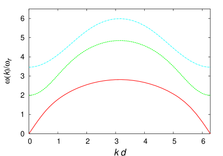
Figure 1: (Color online) Plots of the low-energy Bogoliubov-Bloch modes in the $m=0$ sector. Here, $J=0.1\hbar\omega_{r}$ and $\mu_{0}=50\hbar\omega_{r}$.

The lowest branch corresponds to the Bogoliubov-Bloch axial mode with no radial nodes. This mode has the usual form like $\omega(k)=c_{0}k$ at low momenta. The second branch corresponds to one radial node and starts at $2\omega_{r}$ for $k=0$. The breathing mode has the free-particle dispersion relation and it can be written in terms of the effective mass ($m_{b}^{*}$) of this mode as $\omega_{2}(k)=2\omega_{r}+\hbar k^{2}/2m_{b}^{*}$.

The eigenfunctions corresponding to the low-energy modes are shown in Fig. 2. The eigenfunctions also satisfy the symmetry rule: $\psi_{n_{r},k}(r)=\psi_{n_{r},2\pi-k}(r)$.

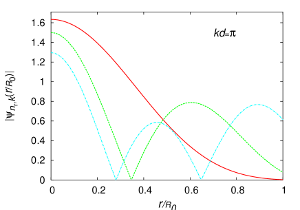
Figure 2: (Color online) Plots of the eigenfunctions of the low-energy modes for $J=0.1\hbar\omega_{r}$ and $\mu_{0}=50\hbar\omega_{r}$.

III Dynamic Structure Factor

The dynamic structure factor is the Fourier transformation of density-density correlation functions. The dynamic structure factor for the layers of quasi-2D condensates can be written as

$$S(q,\omega) = \sum_{j,j^{\prime}}\int d^{2}rd^{2}r^{\prime}dte^{iqd(j-j^{\prime})}e^{i\omega t}$$ (16)

$$\times <\delta\hat{n}_{j}^{{\dagger}}(r,t)\delta\hat{n}_{j^{\prime}}(r^{\prime},0)>.$$

Here, we have used the fact that $q$ is perpendicular to the radial plane. At zero temperature, it can be re-written as

$$S(q,\omega)=\sum_{\alpha}S_{\alpha}(q)\delta(\omega-\omega_{\alpha}(q)),$$ (17)

where weight factor $S_{\alpha}(q)$ is given by

$$S_{\alpha}(q)=|A_{\alpha,q}|^{2}|\psi_{\alpha}(q)|^{2}.$$ (18)

Here, $\psi_{\alpha}(q)=\int d^{2}r\psi_{\alpha,q}({r})$. The weight factors are shown in Fig. 3 as a function of $kd$. The weight factors $S_{\alpha}(q)$ determine how many modes are excited for a given value of $q$. For example, only $n_{r}=1$ and $2$ modes are excited when $qd=1.0$ and other modes are vanishingly small. The weight factors also satisfy the lattice symmetry, $i.e.$, $S_{\alpha}(q)=S_{\alpha}(2\pi-q)$.

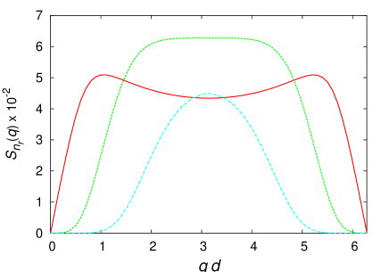
Figure 3: (Color online) Plots of the weight factor for $J=0.1\hbar\omega_{r}$ and $\mu_{0}=50\hbar\omega_{r}$

.

In Fig. 4, we also plot the dynamic structure factor as a function of the Bragg frequency $\omega$ for two values of the Bragg momenta $q$ with fixed $J$ and $\mu_{0}$.

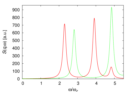
Figure 4: (Color online) Plots of the dynamic structure factor for $kd=\pi/2$ (solid) and $kd=\pi$ (dashed) with fixed $J=0.1\hbar\omega_{r}$ and $\mu_{0}=50\hbar\omega_{r}$.

We find multiple peaks in the dynamic structure factor for a given value of $q$. The location of the peaks correspond to the excitation energy for a given value of $q$ with fixed $J$ and $\mu_{0}$. These peaks show the multibranch nature of the Bogoliubov-Bloch modes.

IV Bragg Spectroscopy

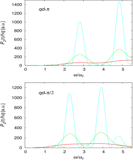
Figure 5: (Color online) Plots of the $P_{z}(t)$ for $J=0.1\hbar\omega_{r}$ and $\mu_{0}=50\hbar\omega_{r}$ for various times $t=0.5T_{r}$(solid), $t=1.0T_{r}$ (dashed) and $t=2.0T_{r}$ (dot-dashed).

The behavior of these multiple peaks in the dynamic structure factor can be resolved in a two-photon Bragg spectroscopy, as shown by Steinhauer et al. mbs2 . The Bragg scattering experiments can be done by applying an additional moving optical potential in the form of $V_{B}(t)=V_{0}\cos(qz-\omega t)$. Here, $V_{0}$ is the intensity of the Bragg pulses. The Bragg potential $V_{B}(t)$ is independent from the static lattice potential $V_{\rm op}$ and it is also much weaker than the lattice potential. We also assume that the excitations are confined within the lowest band, therefore, $\omega$ must be less than the energy gap between the first and second bands. In the two-photon Bragg spectroscopy, the dynamic structure factor can not be measured directly. Actually, the observable in the Bragg scattering experiments is the momentum transferred to the condensate which is related to the dynamic structure factor and reflects the behavior of the quasiparticle energy spectrum. The populations in the quasiparticle states can be controlled by using the two-photon Bragg pulses. When the superfluid is irradiated by an external moving Bragg potential $V_{B}(t)$ the excited states are populated by the quasiparticle with energy $\hbar\omega$ and the momentum $\hbar q$, depending on the value of $q$ and $\omega$ of the Bragg potential $V_{B}(t)$. Due to the axial symmetry, the modes having only zero angular momentum can be excited in the Bragg scattering experiments. Since the Bragg potential is much weaker than the lattice potential, we can treat the scattering process with linear response theory. When the system is subjected to a time-dependent Bragg pulses, the additional interaction term appears in the total energy functional, which is given by,

$$H_{I}(t)=\int dV\psi^{{\dagger}}(r,z,t)[V_{0}\cos(qz-\omega t)]\psi(r,z,t).$$ (19)

The Bragg potential can be approximated as $V_{B}(t)=V_{0}\cos(jqd-\omega t)$ since the atoms scatter off from the condensate by the Bragg pulses from the $j$-th layer. The above interaction energy can be re-written as

$$H_{I}(t)=\sum_{j}\int d^{2}r\psi_{j}^{{\dagger}}(r,t)V_{0}\cos(jqd-\omega t)\psi_{j}(r,t).$$

Following the Refs. tkg1 ; blak , the momentum transfer to the Bose system placed in the optical lattices due the Bragg potential can be calculated analytically and it is given by

$$P_{z}(t) = \sum_{\alpha,k}\hbar k<\hat{b}_{\alpha,k}^{{\dagger}}(t)\hat{b}_{\alpha,k}(t)>=\left(\frac{V_{0}}{2\hbar}\right)^{2}$$ (20)

$$\times \sum_{\alpha}\hbar qS_{\alpha}(\tilde{q})(F_{\alpha}[\omega_{-}t]-F_{\alpha}[\omega_{+}t]),$$

where $\hat{b}_{\alpha,k}(t)$ is the time-evolution of the quasiparticle operator of energy $\hbar\omega_{\alpha}(k)$ and

$$F_{\alpha}[\omega_{\pm}t]=\left(\frac{\sin[(\omega_{\alpha}(q)\pm\omega)t/2]}{(\omega_{\alpha}(q)\pm\omega)/2}\right)^{2}.$$ (21)

In Fig. 5, we plot $P_{z}(t)$ as a function of the Bragg frequency for two values of the Bragg momenta with various time duration. For positive $\omega$ and a given $\tilde{q}$ such that $S_{\alpha}(\tilde{q})$ is maximum, the momentum transferred $P_{z}(t)$ is resonant at the frequencies $\omega=\omega_{\alpha}(q)$. The width of the each peak goes like $2\pi/t$. Figure 5 shows that shape of the $P_{z}(t)$ strongly depends on the time duration of the Bragg pulses. When $t=0.5T_{r}$, the $P_{z}(t)$ is a smooth curve for both values of the Bragg momenta. Here, $T_{r}=2\pi/\omega_{r}$ is the radial trapping period. When $t=1.0T_{r}$, there is a clear evidence of few small peaks developed in the $P_{z}(t)$. When $t=2.0T_{r}$, the multiple peaks in the $P_{z}(t)$ appears sharply. The location of the peaks in Fig. 5 for $t\geq 1.0T_{r}$ are exactly same as in Fig. 4. It implies that $P_{z}(t)\sim S(q,\omega)$ for a long duration of the Bragg pulses. Therefore, in order to resolve the different peaks, the duration of the Bragg pulses should be at least of the order of radial trapping period $T_{r}$. By measuring the $P_{z}$ at different Bragg momenta, it is possible to get information about the MBBS.

V Summary and conclusions

In this work, we have studied excitation energies and the corresponding eigenfunctions of the axial quasiparticles with various discrete radial nodes of an array of weakly coupled quasi-two dimensional Bose condensates. Our discretized hydrodynamic description enables us to produce correctly all low-energy MBBS and the corresponding eigenfunctions by including the mode couplings among different modes within the same angular momentum sector. We have also calculated the dynamic structure factor and the momentum transferred to the system by the Bragg potential. In order to resolve the multiple peaks in the dynamic structure factor, the time duration of the Bragg pulses must be at least of the order of the radial trapping period $T_{r}$. The MBBS can be measured by measuring $P_{z}(t)$ for different values of Bragg momenta, similar to the experiment mbs2 . By measuring the MBBS, one may confirm the effect of the mode coupling on the spectrum.

- (1) B. P. Anderson and M. A. Kasevich, Science 282, 1686 (1998).
- (2) O. Morsch and M. Oberthaler, Rev. Mod. Phys. 78, 179 (2006).
- (3) F. S. Cataliotti, S. Burger, C. Fort, P. Maddaloni, F. Minardi, A. Trombettoni, A. Smerzi, and M. Inguscio, Science 293, 843 (2001).
- (4) S. Burger, F. S. Cataliotti, C. Fort, F. Minardi, M. Inguscio, M. L. Chiofalo, and M. P. Tosi, Phys. Rev. Lett. 86, 4447 (2001).
- (5) M. Ichioka and K. Machida, J. Phys. Soc. Jpn. 72, 2137 (2003).
- (6) D. Jaksch, C. Bruder, J. Cirac, C. W. Gardiner, and P. Zoller, Phys. Rev. Lett. 81, 3108 (1998).
- (7) D. van Oosten, P. van der Straten, and H. T. C. Stoof, Phys. Rev. A 63, 053601 (2001).
- (8) M. Greiner, O. Mandel, T. Esslinger, T. W. Hansch, and I. Bloch, Nature (London) 415, 39 (2002).
- (9) C. Orzel, A. K. Tuchman, M. L. Fenselau, M. Yasuda and M. A. Kasevich, Science 291, 2386 (2001).
- (10) M. Kramer, L. Pitaevskii, and S. Stringari, Phys. Rev. Lett. 88, 180404 (1998).
- (11) C. Fort, F. S. Cataliotti, L. Fallani, F. Ferlaino, P. Maddaloni, and M. Inguscio, Phys. Rev. Lett. 90, 140405 (1998).
- (12) C. Menotti, M. Kramer, L. Pitaevskii, and S. Stringari, Phys. Rev. A 67, 053609 (2003).
- (13) A. M. Rey, P. B. Blakie, G. Pupillo, C. J. Williams, and C. W. Clark, Phys. Rev. A 72, 023407 (2005).
- (14) G. Pupillo, A. M. Rey, and G. G. Bartouni, Phys. Rev. A 74, 013601 (2006).
- (15) O. Zobay and M. Rosenkranz, Phys. Rev. A 74, 053623 (2006).
- (16) K. Berg-Sorenson and K. Molmer, Phys. Rev. A 58, 1480 (1998).
- (17) J. Javannainen, Phys. Rev. A 60, 4902 (1999).
- (18) M. Machalom, C. J. Pethick, and H. Smith, Phys. Rev. A 67, 053613 (2003).
- (19) E. Taylor and E. Zaremba, Phys. Rev. A 68, 053611 (2003).
- (20) T. K. Ghosh and K. Machida, Phys. Rev. A 72, 053623 (2006).
- (21) E. Zaremba, Phys. Rev. A 57, 518 (1998).
- (22) P. O. Fedichev and G. V. Shlyapnikov, Phys. Rev. A 63, 045601 (2001).
- (23) J. Stenger, S. Inouye, A. P. Chikkatur, D. M. Stamper-Kurn, D. E. Pritchard, and W. Ketterle, Phys. Rev. Lett. 82, 4569 (1999); D. M. Stamper-Kurn, A. P. Chikkatur, A. Gorlitz, S. Inouye, S. Gupta, D. E. Pritchard, and W. Ketterle, Phys. Rev. Lett. 83, 2876 (1999).
- (24) J. Steinhauer, N. Katz, R. Orezi, N. Davidson, C. Tozzo and F. Dalfovo, Phys. Rev. Lett. 90, 060404 (2003).
- (25) S. Richard, F. Gerbier, J. H. Thywissen, M. Hugbart, P. Bouyer, and A. Aspect, Phys. Rev. Lett. 91, 010405 (2003).
- (26) F. Gerbier, J. H. Thywissen, S. Richard, M. Hugbart, P. Bouyer, and A. Aspect, Phys. Rev. A 67, 051602 (2003).
- (27) S. R. Muniz, D. S. Nayak, and C. Raman, Phys. Rev. A 73, 041605(R) (2006).
- (28) J. P. Martikainen and H. T. C. Stoof, Phys. Rev. A 69, 023608 (2004).
- (29) J. P. Martikainen and H. T. C. Stoof, Phys. Rev. A 68, 013610 (2003).
- (30) M. Fleesser, Andras Csordas, P. Szepfalusy, and R. Graham, Phys. Rev. A 56, 2533(R) (1997); P. Ohberg, E. L. Surkov, I. Tittonen, S. Stenholm, M. Wilkens, and G. V. Shlyapnikov, Phys. Rev. A 56, 3346(R) (1997).
- (31) T. K. Ghosh, Int. J Mod. Phy. B 20, 5443 (2006).
- (32) P. B. Blakie, R. J. Ballagh, and C. W. Gardiner, Phys. Rev. A 65, 033602 (2002).