Semiconductor quantum dots in high magnetic fields: The composite-fermion view

Abstract

We review and extend the composite fermion theory for semiconductor quantum dots in high magnetic fields. The mean-field model of composite fermions is unsatisfactory for the qualitative physics at high angular momenta. Extensive numerical calculations demonstrate that the microscopic CF theory, which incorporates interactions between composite fermions, provides an excellent qualitative and quantitative account of the quantum dot ground state down to the largest angular momenta studied, and allows systematic improvements by inclusion of mixing between composite fermion Landau levels (called $\Lambda$ levels).

I Introduction

The system of interacting electrons confined to a two dimensional quantum dot and exposed to a strong magnetic field has been a subject of intense theoretical study for over two decades. review ; Yoshioka ; Girvin ; Dev ; Beenakker93 ; Yang ; Tapash ; Xie ; Hawrylak ; Kawamura ; Kamilla ; Seki ; Manninen ; Cappelli ; Landman ; Ruan ; Maksym ; Harju ; RQLC ; Rei2 ; Toreblad ; Cnell ; Rei5 ; Peeters2 ; Muller Such quantum dots have been realized and studied in the laboratory. Expt1 ; Expt2 ; Expt3 ; Expt4 Exact diagonalization studies show that the ground states are strongly correlated, and the aim of theory is to achieve a satisfactory understanding of the correlations. It is also of interest to understand how this ties into our understanding of the FQHE, Tsui obtained in the thermodynamic limit without confinement.

The CF theory has been applied to parabolic quantum dots subjected to a strong magnetic field. The plot of ground state energy as a function of the angular momentum ($L$) has a rich structure. In particular, downward cusps appear at certain values of $L$, which are consequently especially favorable. Early studies Dev ; Beenakker93 ; Kawamura ; Kamilla demonstrated the CF theory to be promising. Specifically, a “mean-field model,” in which the composite fermions are taken as noninteracting particles at an effective angular momentum $L^{*}$, with their mass or the cyclotron energy treated as a phenomenological parameter, predicts cusps in the energy at certain magic angular momenta; these predictions are in agreement with the actual cusp positions in exact diagonalization studies at small angular momenta $L$, but discrepancies appear at large $L$. Seki ; Landman Further work Jeon ; Jeon2 showed that these discrepancies are special to the mean-field model of the CF theory. A perfect agreement between the actual and the predicted cusp positions was obtained when the CF energies were calculated from microscopic wave functions. One of the surprising aspects was the success of the CF theory even at the largest angular momenta studied, which appears, at first, to be at odds with the classical crystal-like correlations found in exact diagonalization studies. Seki ; Maksym While both composite fermions and the crystal are generated by the repulsive interaction between electrons, the implicit assumption had been that one excluded the other. The work in Ref. Jeon2, showed that no logical inconsistency exists between the simultaneous formations of composite fermions and crystal-like structures at low fillings, and, furthermore, the formation of composite fermions itself induces crystal structure at low fillings. This crystal has been shown to be very well described as a crystal of composite fermions. CFcrystal ; onefifth

The aim of this paper is to review and extend the CF theory of quantum dots in high magnetic fields, and also provide many details left out in earlier papers. Section II briefly outlines the basics of the CF theory for quantum dot states, giving explicit wave functions for some simple cases. Section III describes the numerical methods (exact diagonalization, Lanczos, and CF diagonalization). The mean-field CF model is discussed in Sec. IV, and the “zeroth-order” CF diagonalization in Sec. V. Section VI illustrates how the results are improved by going to higher orders in the CF theory. The paper is concluded in Sec. VII.

II The composite-fermion basics for quantum dots

Following the standard practice, we assume below parabolic confinement. This should be a good approximation for most quantum dots at low energies, and simplifies calculations because of the availability of exact solutions for single particle eigenstates. The Hamiltonian of interest is

$$H{=}\sum_{j}\frac{1}{2m_{b}}\left(\mbox{\boldmath$p$}_{j}+\frac{e}{c}\mbox{\boldmath$A$}_{j}\right)^{2}+\sum_{j}\frac{m_{b}}{2}\omega_{0}^{2}r_{j}^{2}+\sum_{j<k}\frac{e^{2}}{\epsilon r_{jk}},$$ (1)

where $m_{b}$ is the band mass of the electron, $\omega_{0}$ is a measure of the strength of the confinement, $\epsilon$ is the dielectric constant of the host semiconductor, and $r_{jk}\equiv|\mbox{\boldmath$r$}_{j}-\mbox{\boldmath$r$}_{k}|$. We will specialize to the case of very large magnetic fields, when $\omega_{c}\equiv eB/m_{b}c\gg\omega_{0}$. Only the lowest Landau level (LL) is relevant in this limit. In that limit, at each angular momentum the eigenenergy neatly separates into a confinement part and an interaction part:

$$E(L)=E_{c}(L)+V(L),$$ (2)

where $E_{c}(L)=(\hbar/2)[\Omega-\omega_{c}]L$, relative to the lowest LL, with $\Omega^{2}\equiv\omega_{c}^{2}+4\omega_{0}^{2}$, and $V(L)$ is the interaction energy of electrons without confinement, but with the magnetic length replaced by an effective magnetic length given by $\ell\equiv\sqrt{\hbar/m_{b}\Omega}$. In the following, we will consider only $V$ as a function of the angular momentum $L$; it must be remembered, however, that the confinement part must be added to determine the global ground state.

(a)

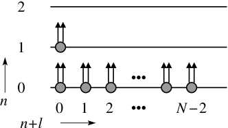
(b)

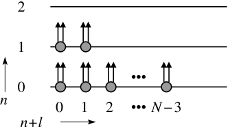
(c)

Figure 1: Schematic depiction of (a) $[N,0]$, (b) $[N-1,1]$, and (c) $[N-2,2]$ states in terms of composite fermions carrying two vortices ($2p=2$). The composite fermions are shown as electrons with two arrows, where the arrows represent the vortices bound to composite fermions. The labels $n$ and $l$ denote the $\Lambda$ level (CF Landau level) index and the angular momentum of the composite fermion, respectively.

In the CF theory, Dev ; Kawamura ; Jain the interacting state of electrons in the lowest LL at angular momentum $L$ is mapped into the noninteracting electron state at $L^{*}$, where

$$L=L^{*}+pN(N-1)\;,$$ (3)

$N$ is the number of electrons, and $p$ is an integer. The wave functions

$$\Psi^{L}_{\alpha}={\cal P}_{\rm LLL}\prod_{j<k}(z_{j}-z_{k})^{2p}\Phi^{L^{*}}_{\alpha}$$ (4)

give ansatz wave functions for interacting electrons at $L$ in terms of the known wave functions of noninteracting electrons at $L^{*}$. Here $\Phi^{L^{*}}_{\alpha}$ are the wave functions for noninteracting electrons at $L^{*}$ (which in general occupy several Landau levels), $\alpha=1,2,\cdots,D^{*}$ labels the different states, $z_{j}=x_{j}-iy_{j}$ denotes the position of the $j$th electron, ${\cal P}_{\rm LLL}$ indicates projection into the lowest LL, $\Psi_{\alpha}^{L}$ are basis functions for interacting electrons at $L$, and $D^{*}$ is the dimension of the CF basis. We will restrict $\Phi_{\alpha}^{L^{*}}$ to states with the lowest kinetic energy at $L^{*}$, and choose $p$ so as to have the smallest dimension for the basis. The composite fermions carrying $2p$ vortices are labeled ^2pCF’s. At certain values of $L$, the above prescription produces only one state ($D^{*}=1$), which is the CF theory’s answer for the ground state. In the notation of Ref. Kawamura, , this is a compact state, denoted by $[N_{0},N_{1},\cdots]$, with $N_{j}$ composite fermions compactly occupying the innermost angular momentum orbitals of the $j$th CF level. At other values of $L$, when there are many CF basis states ($D^{*}>1$), we diagonalize the Coulomb Hamiltonian in the CF basis to obtain the ground state, using methods described earlier. Kamilla ; Mandal For any $N$, there are many values of $L$ where the CF theory gives a unique answer, but in general, $D^{*}$ increases with $N$.

II.1 Examples of CF bases

Construction of the CF basis is in principle straightforward. We consider some explicit examples.

In many cases, the CF basis consists of a unique wave function, which simplifies the analysis tremendously. The simplest wave function is the one for one filled $\Lambda$ level (CF Landau level), shown schematically in Fig. 1(a):

$$\Psi = A\left[\prod_{i=1}^{N}z_{i}^{i-1}\right]\Phi_{1}^{2p}$$ (5)

$$= \prod_{j<k}(z_{j}-z_{k})^{2p+1}e^{-\sum_{l=1}^{N}|z_{l}|^{2}/4},$$

where $A$ denotes an antisymmetric Slater determinant, i.e.

$$A\left[\prod_{i=1}^{N}z_{i}^{i-1}\right] = \left|\begin{matrix}1&1&\ldots&1\\ z_{1}&z_{2}&\ldots&z_{N}\\ \vdots&\vdots&\ddots&\vdots\\ z_{1}^{N-1}&z_{2}^{N-1}&\ldots&z_{N}^{N-1}\end{matrix}\right|$$ (6)

$$= \prod_{j<k}(z_{j}-z_{k})$$

and

$$\Phi_{1}^{2p}\equiv\prod_{j<k}(z_{j}-z_{k})^{2p}e^{-\sum_{l=1}^{N}|z_{l}|^{2}/4}.$$ (7)

It corresponds to $L=(2p+1)N(N-1)/2$. It is identical to the Laughlin wave function.

The state $[N-1,1]$ at $L=(2p+1)N(N-1)/2-N$, shown in Fig. 1(b), represents the wave function

$$\Psi={\cal P}_{\rm LLL}A\left[z_{1}^{*}\cdot\prod_{i=2}^{N}z_{i}^{i-2}\right]\Phi_{1}^{2p}.$$ (8)

This state has been interpreted as a charged quasiparticle excitation of the $\nu=1/(2p+1)$ FQHE state. QP The $[N-2,2]$ state (Fig. 1(c)) occurs at $L=(2p+1)N(N-1)/2-2(N-1)$, and has the wave function

$$\Psi={\cal P}_{\rm LLL}A\left[z_{1}^{*}\cdot z_{2}z_{2}^{*}\cdot\prod_{i=3}^{N}z_{i}^{i-3}\right]\Phi_{1}^{2p}.$$ (9)

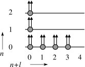
(a)

  

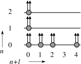
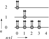
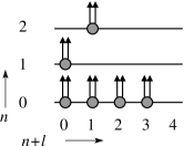
(b)

Figure 2: Schematic depiction of basis states at (a) $L=33$; (b) $L=34$ for $N=6$ particles.

For many angular momenta, the basis contains more than one state. For six composite fermions at $L=33$ we have two compact states [3,3] and [4,1,1], as depicted schematically in Fig. 2(a). The basis functions are given by

$$\Psi_{1}^{L=33} = {\cal P}_{\rm LLL}A\left[\prod_{i=1}^{3}\left(z_{i}^{*}z_{i}^{i-1}\right)\cdot\prod_{i=4}^{6}z_{i}^{i-4}\right]\Phi_{1}^{2},$$ (10a)

$$\Psi_{2}^{L=33} = {\cal P}_{\rm LLL}A\left[(z_{1}^{*})^{2}\cdot z_{2}^{*}\cdot\prod_{i=3}^{6}z_{i}^{i-3}\right]\Phi_{1}^{2}.$$ (10b)

These have the same CF kinetic energy, leading to $D^{*}=2$ at $L=33$. The five basis states at $L=34$ are shown in Fig. 2(b), derived from either [4,1,1] or [3,3] by increasing the angular momentum by one unit. The corresponding basis functions are written as

$$\Psi_{1}^{L=34} = {\cal P}_{\rm LLL}A\left[\eta_{1}^{-1}(z_{1})\cdot\eta_{1}^{0}(z_{2})\cdot\eta_{1}^{1}(z_{3})\cdot\eta_{0}^{0}(z_{4})\cdot\eta_{0}^{1}(z_{5})\cdot\eta_{0}^{3}(z_{6})\right]\Phi_{1}^{2},$$ (11a)

$$\Psi_{2}^{L=34} = {\cal P}_{\rm LLL}A\left[\eta_{1}^{-1}(z_{1})\cdot\eta_{1}^{0}(z_{2})\cdot\eta_{1}^{2}(z_{3})\cdot\eta_{0}^{0}(z_{4})\cdot\eta_{0}^{1}(z_{5})\cdot\eta_{0}^{2}(z_{6})\right]\Phi_{1}^{2},$$ (11b)

$$\Psi_{3}^{L=34} = {\cal P}_{\rm LLL}A\left[\eta_{2}^{-2}(z_{1})\cdot\eta_{1}^{-1}(z_{2})\cdot\eta_{0}^{0}(z_{3})\cdot\eta_{0}^{1}(z_{4})\cdot\eta_{0}^{2}(z_{5})\cdot\eta_{0}^{4}(z_{6})\right]\Phi_{1}^{2},$$ (11c)

$$\Psi_{4}^{L=34} = {\cal P}_{\rm LLL}A\left[\eta_{2}^{-2}(z_{1})\cdot\eta_{1}^{0}(z_{2})\cdot\eta_{0}^{0}(z_{3})\cdot\eta_{0}^{1}(z_{4})\cdot\eta_{0}^{2}(z_{5})\cdot\eta_{0}^{3}(z_{6})\right]\Phi_{1}^{2},$$ (11d)

$$\Psi_{5}^{L=34} = {\cal P}_{\rm LLL}A\left[\eta_{2}^{-1}(z_{1})\cdot\eta_{1}^{-1}(z_{2})\cdot\eta_{0}^{0}(z_{3})\cdot\eta_{0}^{1}(z_{4})\cdot\eta_{0}^{2}(z_{5})\cdot\eta_{0}^{3}(z_{6})\right]\Phi_{1}^{2}.$$ (11e)

Here

$$\eta_{n}^{l}(z)\equiv z^{l}L_{n}^{l}(zz^{*}/2)$$ (12)

with $L_{n}^{l}(x)$ being an associated Laguerre polynomial.

$L$	$D$	$D^{*}$	$V_{\rm ex}$	$V_{\rm CF}$	$L$	$D$	$D^{*}$	$V_{\rm ex}$	$V_{\rm CF}$	$L$	$D$	$D^{*}$	$V_{\rm ex}$	$V_{\rm CF}$	$L$	$D$	$D^{*}$	$V_{\rm ex}$	$V_{\rm CF}$
9	3	1	1.93481	1.93462(17)	39	378	2	0.88879	0.88986(5)	69	2178	2	0.66433	0.66487(3)	99	6528	2	0.54944	0.54965(1)
10	5	1	1.78509	1.78496(21)	40	411	4	0.88032	0.88147(7)	70	2280	1	0.65131	0.65168(2)	100	6736	4	0.54748	0.54790(3)
11	6	2	1.78509	1.78487(21)	41	441	6	0.87275	0.87410(5)	71	2376	2	0.65131	0.65167(4)	101	6936	6	0.54581	0.54625(4)
12	9	1	1.68518	1.68616(7)	42	478	1	0.84446	0.84822(7)	72	2484	1	0.64803	0.65220(4)	102	7153	1	0.53846	0.53874(2)
13	11	2	1.64157	1.64407(27)	43	511	1	0.84446	0.84813(9)	73	2586	2	0.64520	0.64678(7)	103	7361	1	0.53846	0.53879(3)
14	15	1	1.50066	1.50174(20)	44	551	2	0.83722	0.84177(10)	74	2700	1	0.63324	0.63361(3)	104	7586	2	0.53662	0.53713(3)
15	18	2	1.50066	1.50157(7)	45	588	2	0.83079	0.83160(12)	75	2808	2	0.63324	0.63362(2)	105	7803	2	0.53505	0.53527(2)
16	23	4	1.46397	1.46424(28)	46	632	1	0.80616	0.80683(7)	76	2928	4	0.63023	0.63088(4)	106	8037	1	0.52812	0.52825(2)
17	27	6	1.42958	1.42999(43)	47	672	2	0.80616	0.80680(8)	77	3042	6	0.62764	0.62843(1)	107	8262	2	0.52812	0.52825(4)
18	34	1	1.30573	1.31078(10)	48	720	1	0.79987	0.80871(4)	78	3169	1	0.61660	0.61727(2)	108	8505	1	0.52638	0.52761(3)
19	39	1	1.30573	1.31054(25)	49	764	2	0.79434	0.79747(11)	79	3289	1	0.61660	0.61732(5)	109	8739	2	0.52490	0.52543(2)
20	47	2	1.27825	1.28375(7)	50	816	1	0.77263	0.77345(10)	80	3422	2	0.61382	0.61499(3)	110	8991	1	0.51834	0.51850(2)
21	54	2	1.24416	1.24456(13)	51	864	2	0.77263	0.77337(5)	81	3549	2	0.61143	0.61186(7)	111	9234	2	0.51834	0.51850(2)
22	64	1	1.17779	1.17793(7)	52	920	4	0.76711	0.76815(4)	82	3689	1	0.60120	0.60147(2)	112	9495	4	0.51670	0.51700(4)
23	72	2	1.17779	1.17792(9)	53	972	6	0.76229	0.76350(7)	83	3822	2	0.60120	0.60146(3)	113	9747	6	0.51530	0.51570(2)
24	84	1	1.15660	1.16365(10)	54	1033	1	0.74297	0.74506(4)	84	3969	1	0.59863	0.60135(5)	114	10018	1	0.50910	0.50934(4)
25	94	2	1.13775	1.14169(19)	55	1089	1	0.74297	0.74507(2)	85	4109	3	0.59642	0.59747(5)	115	10279	1	0.50910	0.50934(2)
26	108	1	1.08038	1.08168(7)	56	1154	2	0.73807	0.74093(4)	86	4263	1	0.58690	0.58720(5)	116	10559	2	0.50754	0.50795(3)
27	120	2	1.08038	1.08170(19)	57	1215	2	0.73381	0.73440(4)	87	4410	2	0.58690	0.58719(6)	117	10830	2	0.50622	0.50640(1)
28	136	4	1.06508	1.06589(12)	58	1285	1	0.71648	0.71693(6)	88	4571	4	0.58451	0.58502(4)	118	11120	1	0.50033	0.50043(2)
29	150	6	1.05089	1.05181(17)	59	1350	2	0.71648	0.71700(10)	89	4725	6	0.58246	0.58306(4)	119	11400	2	0.50033	0.50045(5)
30	169	1	1.00340	1.00915(10)	60	1425	1	0.71209	0.71838(9)	90	4894	1	0.57358	0.57404(2)	120	11700	1	0.49885	0.49971(2)
31	185	1	1.00340	1.00922(11)	61	1495	2	0.70829	0.71053(5)	91	5055	1	0.57358	0.57402(3)	121	11990	2	0.49759	0.49801(4)
32	206	2	0.99110	0.99756(13)	62	1575	1	0.69263	0.69317(2)	92	5231	2	0.57135	0.57208(4)	122	12300	1	0.49199	0.49212(1)
33	225	2	0.97949	0.98037(14)	63	1650	2	0.69263	0.69316(4)	93	5400	2	0.56944	0.56976(3)	123	12600	2	0.49199	0.49211(2)
34	249	1	0.94091	0.94152(6)	64	1735	4	0.68868	0.68955(3)	94	5584	1	0.56112	0.56130(1)	124	12920	4	0.49059	0.49084(2)
35	270	2	0.94091	0.94159(10)	65	1815	6	0.68526	0.68631(6)	95	5760	2	0.56112	0.56132(2)	125	13230	6	0.48940	0.48969(4)
36	297	1	0.93079	0.94124(14)	66	1906	1	0.67102	0.67223(3)	96	5952	1	0.55903	0.56084(3)	126	13561	1	0.48406	0.48423(2)
37	321	2	0.92164	0.92557(8)	67	1991	1	0.67102	0.67224(8)	97	6136	2	0.55725	0.55797(2)	127	13881	1	0.48406	0.48422(1)
38	351	1	0.88879	0.88988(8)	68	2087	2	0.66743	0.66920(6)	98	6336	1	0.54944	0.54965(1)	128	14222	2	0.48273	0.48305(3)

Table 1: Comparison between the CF and the exact energies ($V_{\rm CF}$ and $V_{\rm ex}$) for $N=4$. The symbols in this and the following tables have the following meaning: $L$ is the angular momentum; $D$ is the dimension of the full lowest LL Fock space; and $D^{*}$ is the dimension of the CF basis. The energies are in units of $e^{2}/\epsilon\ell$, where $\epsilon$ is the dielectric constant of the background semiconductor and $\ell=\sqrt{\hbar c/eB}$ is the magnetic length.

$L$	$D$	$D^{*}$	$V_{\rm ex}$	$V_{\rm CF}$	$L$	$D$	$D^{*}$	$V_{\rm ex}$	$V_{\rm CF}$	$L$	$D$	$D^{*}$	$V_{\rm ex}$	$V_{\rm CF}$	$L$	$D$	$D^{*}$	$V_{\rm ex}$	$V_{\rm CF}$
13	3	1	3.20199	3.20205(29)	39	603	4	1.80374	1.80580(23)	65	5260	1	1.36535	1.36767(8)	91	21224	1	1.15674	1.16090(6)
14	5	1	3.05525	3.05557(34)	40	674	1	1.75246	1.75282(18)	66	5608	2	1.36535	1.36759(22)	92	22204	2	1.15054	1.15487(9)
15	7	1	2.91866	2.91868(43)	41	748	3	1.75246	1.75288(31)	67	5969	4	1.35517	1.35697(15)	93	23212	4	1.14579	1.14689(10)
16	10	3	2.91866	2.91927(60)	42	831	1	1.72570	1.72659(20)	68	6351	7	1.34694	1.34856(13)	94	24260	2	1.14172	1.14284(19)
17	13	1	2.83078	2.83119(66)	43	918	2	1.71164	1.71548(21)	69	6747	11	1.33969	1.34091(8)	95	25337	1	1.12540	1.12654(8)
18	18	1	2.69089	2.69274(9)	44	1014	5	1.69696	1.70152(21)	70	7166	1	1.31464	1.31980(9)	96	26455	6	1.12540	1.12645(4)
19	23	3	2.66332	2.66466(35)	45	1115	1	1.64891	1.65141(11)	71	7599	1	1.31464	1.31964(14)	97	27604	2	1.11969	1.12238(3)
20	30	1	2.53676	2.53706(42)	46	1226	2	1.64894	1.65148(25)	72	8056	2	1.30556	1.31141(4)	98	28796	1	1.11535	1.12055(7)
21	37	3	2.53676	2.53710(58)	47	1342	4	1.63127	1.63345(10)	73	8529	4	1.29822	1.29938(14)	99	30020	4	1.11166	1.11286(10)
22	47	1	2.42979	2.43092(41)	48	1469	7	1.61635	1.61828(21)	74	9027	2	1.29148	1.29258(16)	100	31289	1	1.09648	1.09737(7)
23	57	2	2.41248	2.41695(62)	49	1602	11	1.60206	1.60277(31)	75	9542	1	1.26920	1.27036(9)	101	32591	3	1.09648	1.09738(7)
24	70	5	2.37282	2.37632(85)	50	1747	1	1.56144	1.56666(3)	76	10083	6	1.26920	1.27029(12)	102	33940	1	1.09120	1.09795(6)
25	84	1	2.24724	2.24910(16)	51	1898	1	1.56144	1.56655(18)	77	10642	2	1.26100	1.26384(13)	103	35324	2	1.08722	1.09060(9)
26	101	2	2.23577	2.23796(46)	52	2062	2	1.54661	1.55380(9)	78	11229	1	1.25446	1.25857(11)	104	36756	5	1.08384	1.08634(13)
27	119	4	2.20889	2.21135(19)	53	2233	4	1.53301	1.53401(14)	79	11835	4	1.24894	1.25059(9)	105	38225	1	1.06968	1.07123(3)
28	141	7	2.17424	2.17563(68)	54	2418	2	1.51746	1.51797(7)	80	12470	1	1.22816	1.22917(4)	106	39744	2	1.06968	1.07111(20)
29	164	11	2.13794	2.13853(73)	55	2611	1	1.48714	1.48776(10)	81	13125	3	1.22816	1.22895(9)	107	41301	4	1.06477	1.06622(4)
30	192	1	2.02725	2.03083(17)	56	2818	6	1.48714	1.48809(22)	82	13811	1	1.22072	1.22684(12)	108	42910	7	1.06110	1.06269(2)
31	221	1	2.02725	2.03097(27)	57	3034	2	1.47396	1.47634(15)	83	14518	2	1.21493	1.21855(9)	109	44559	11	1.05798	1.05946(3)
32	255	2	1.99957	2.00534(11)	58	3266	1	1.46155	1.46315(4)	84	15257	5	1.21000	1.21295(24)	110	46262	1	1.04475	1.04795(4)
33	291	4	1.96593	1.96741(23)	59	3507	4	1.45293	1.45490(12)	85	16019	1	1.19085	1.19276(10)	111	48006	1	1.04475	1.04789(4)
34	333	2	1.92313	1.92424(17)	60	3765	1	1.42240	1.42328(17)	86	16814	2	1.19085	1.19276(3)	112	49806	2	1.04018	1.04349(8)
35	377	1	1.87634	1.87694(30)	61	4033	3	1.42240	1.42339(17)	87	17633	4	1.18408	1.18585(3)	113	51649	4	1.03678	1.03755(7)
36	427	6	1.87634	1.87662(29)	62	4319	1	1.41061	1.41445(13)	88	18487	7	1.17885	1.18048(10)	114	53550	2	1.03389	1.03495(8)
37	480	2	1.85037	1.85214(37)	63	4616	2	1.40132	1.40514(12)	89	19366	11	1.17438	1.17585(12)
38	540	1	1.81607	1.81678(9)	64	4932	5	1.39332	1.39690(36)	90	20282	1	1.15674	1.16095(10)

Table 2: Comparison between the CF and the exact energies ($V_{\rm CF}$ and $V_{\rm ex}$) for $N=5$.

$L$	$D$	$D^{*}$	$V_{\rm ex}$	$V_{\rm CF}$	$L$	$D$	$D^{*}$	$V_{\rm ex}$	$V_{\rm CF}$	$L$	$D$	$D^{*}$	$V_{\rm ex}$	$V_{\rm CF}$	$L$	$D$	$D^{*}$	$V_{\rm ex}$	$V_{\rm CF}$
19	5	1	4.52568	4.52563(84)	52	2702	10	2.69635	2.70122(14)	85	38677	1	2.06506	2.06929(9)	118	216705	9	1.75766	1.76108(13)
20	7	1	4.39138	4.39214(47)	53	3009	5	2.66882	2.67239(64)	86	41134	5	2.06506	2.06911(12)	119	226479	3	1.74584	1.75185(20)
21	11	1	4.26439	4.26485(31)	54	3331	2	2.63071	2.63357(25)	87	43752	2	2.05433	2.05522(17)	120	236534	1	1.73124	1.73566(10)
22	14	3	4.26439	4.26557(67)	55	3692	1	2.58540	2.58872(13)	88	46461	9	2.04622	2.04944(24)	121	247010	3	1.73124	1.73575(13)
23	20	2	4.15579	4.15623(25)	56	4070	5	2.58541	2.58807(20)	89	49342	3	2.02791	2.03308(20)	122	257783	8	1.72727	1.73012(18)
24	26	1	4.05541	4.05721(58)	57	4494	2	2.55188	2.55252(31)	90	52327	1	2.00538	2.00952(20)	123	269005	2	1.72031	1.72323(11)
25	35	1	3.92152	3.92355(10)	58	4935	9	2.54880	2.55221(22)	91	55491	3	2.00538	2.00969(35)	124	280534	4	1.70935	1.71436(23)
26	44	3	3.90771	3.90868(73)	59	5427	3	2.51327	2.51647(68)	92	58767	8	1.99893	2.00142(44)	125	292534	1	1.69562	1.69987(6)
27	58	2	3.79370	3.79420(72)	60	5942	1	2.47124	2.47423(27)	93	62239	2	1.98517	1.98615(10)	126	304865	2	1.69562	1.69984(3)
28	71	5	3.79370	3.79447(29)	61	6510	3	2.47124	2.47420(61)	94	65827	4	1.97151	1.97625(13)	127	317683	5	1.69191	1.69581(16)
29	90	2	3.69049	3.69200(92)	62	7104	8	2.45835	2.45998(31)	95	69624	1	1.95061	1.95495(22)	128	330850	9	1.68552	1.68900(11)
30	110	1	3.56719	3.56824(40)	63	7760	2	2.42388	2.42431(35)	96	73551	2	1.95061	1.95514(20)	129	344534	1	1.67503	1.68120(11)
31	136	3	3.56264	3.56580(66)	64	8442	4	2.40947	2.41278(12)	97	77695	5	1.94470	1.94832(11)	130	358579	2	1.66210	1.66513(14)
32	163	7	3.52932	3.53013(84)	65	9192	1	2.37120	2.37547(20)	98	81979	9	1.93471	1.93824(39)	131	373165	4	1.66210	1.66519(27)
33	199	2	3.41858	3.41952(30)	66	9975	2	2.37120	2.37513(14)	99	86499	1	1.91890	1.92278(10)	132	388138	7	1.65863	1.66131(18)
34	235	4	3.40210	3.40435(61)	67	10829	5	2.35951	2.36237(52)	100	91164	2	1.90010	1.90348(12)	133	403670	12	1.65264	1.65522(33)
35	282	1	3.28942	3.29204(19)	68	11720	9	2.34182	2.34476(24)	101	96079	4	1.90010	1.90329(29)	134	419609	18	1.64273	1.64584(15)
36	331	2	3.28587	3.29094(28)	69	12692	1	2.30954	2.31154(17)	102	101155	7	1.89472	1.89762(22)	135	436140	1	1.63050	1.63876(7)
37	391	5	3.25902	3.26178(31)	70	13702	2	2.28245	2.28574(35)	103	106491	12	1.88550	1.88831(53)	136	453091	1	1.63050	1.63878(14)
38	454	9	3.21604	3.21752(83)	71	14800	4	2.28245	2.28624(68)	104	111999	18	1.87118	1.87361(51)	137	470660	2	1.62723	1.63454(7)
39	532	1	3.11031	3.11221(29)	72	15944	7	2.27239	2.27584(8)	105	117788	1	1.85328	1.86170(17)	138	488678	3	1.62159	1.62801(1)
40	612	2	3.06846	3.07277(56)	73	17180	12	2.25596	2.25924(17)	106	123755	1	1.85328	1.86180(13)	139	507334	4	1.61221	1.61833(7)
41	709	4	3.06846	3.07263(46)	74	18467	18	2.23266	2.23432(46)	107	130019	2	1.84828	1.85551(23)	140	526461	2	1.60064	1.60352(19)
42	811	7	3.03681	3.03929(84)	75	19858	1	2.20188	2.20932(19)	108	136479	3	1.83963	1.84614(12)	141	546261	1	1.60064	1.60808(6)
43	931	12	3.00162	3.00288(91)	76	21301	1	2.20188	2.20944(22)	109	143247	4	1.82642	1.83222(16)	142	566547	10	1.59756	1.60028(38)
44	1057	18	2.95620	2.95640(61)	77	22856	2	2.19230	2.19868(34)	110	150224	2	1.80978	1.81276(9)	143	587535	5	1.59225	1.59806(30)
45	1206	1	2.86015	2.86444(21)	78	24473	3	2.17671	2.18392(17)	111	157532	1	1.80978	1.81507(10)	144	609040	2	1.58332	1.58980(9)
46	1360	1	2.86015	2.86427(33)	79	26207	4	2.15698	2.16067(26)	112	165056	10	1.80521	1.80836(23)	145	631269	1	1.57236	1.57642(6)
47	1540	2	2.83682	2.84249(21)	80	28009	2	2.13038	2.13341(12)	113	172929	5	1.79729	1.80306(20)	146	654039	5	1.57236	1.57638(12)
48	1729	3	2.80401	2.81080(37)	81	29941	1	2.12855	2.13017(15)	114	181038	2	1.78476	1.79071(14)	147	677571	2	1.56945	1.57511(12)
49	1945	4	2.76617	2.77264(33)	82	31943	10	2.12260	2.12620(49)	115	189509	1	1.76921	1.77344(27)	148	701661	9	1.56444	1.56751(15)
50	2172	2	2.71674	2.72205(36)	83	34085	5	2.10896	2.11372(47)	116	198230	5	1.76921	1.77351(18)
51	2432	1	2.69635	2.70145(36)	84	36308	2	2.08934	2.09405(13)	117	207338	2	1.76490	1.76806(14)

Table 3: Comparison between the CF and the exact energies ($V_{\rm CF}$ and $V_{\rm ex}$) for $N=6$.

The projection into the lowest LL is accomplished by the method outlined in the literature. Kamilla To give a simple example, consider the state $[N-1,1]$ state in Eq. (8). We use the identity (apart from the constant factor),

$$A\left[z_{1}^{*}\cdot\prod_{i=2}^{N}z_{i}^{i-2}\right]\prod_{j<k}(z_{j}-z_{k})^{2p}=A\left[z_{1}^{*}J_{1}^{p}\cdot\prod_{i=2}^{N}(z_{i}^{i-2}J_{i}^{p})\right]$$ (13)

with

$$J_{i}\equiv\prod_{j(\neq i)}(z_{i}-z_{j})$$ (14)

and project each element to the lowest LL, resulting in

$$\Psi=e^{-\sum_{l=1}^{N}|z_{l}|^{2}/4}A\left[{\cal P}_{\rm LLL}(z_{1}^{*}J_{1}^{p})\cdot\prod_{i=2}^{N}{\cal P}_{\rm LLL}(z_{i}^{i-2}J_{i}^{p})\right].$$ (15)

The final step is achieved by placing all of the $z_{j}^{*}$’s to the left, and substituting $2\partial/\partial z_{j}$ into $z_{j}^{*}$ with the assumption that the derivatives do not act on the Gaussian factor. Jain ; Girvin2 The resulting wave function is then given by

$$\Psi=A\left[\sum_{j\neq 1}\frac{1}{z_{1}-z_{j}}\cdot\prod_{i=2}^{N}z_{i}^{i-2}\right]\Phi_{1}^{2p}.$$ (16)

Lowest LL projection of other can be accomplished similarly, although the details are more complicated.

$L$	$D$	$D^{*}$	$V_{\rm ex}$	$V_{\rm CF}$	$L$	$D$	$D^{*}$	$V_{\rm ex}$	$V_{\rm CF}$	$L$	$D$	$D^{*}$	$V_{\rm ex}$	$V_{\rm CF}$	$L$	$D$	$D^{*}$	$V_{\rm ex}$	$V_{\rm CF}$
26	7	1	6.04656	6.04681(54)	52	2093	2	4.26158	4.26561(73)	78	34082	1	3.42977	3.43487(25)	104	225286	29	2.94535	2.94866(61)
27	11	1	5.92221	5.92332(86)	53	2400	5	4.23491	4.23965(35)	79	37108	9	3.41304	3.41884(47)	105	239691	1	2.91436	2.93077(20)
28	15	1	5.80240	5.80314(97)	54	2738	9	4.19836	4.20134(65)	80	40340	3	3.37769	3.38473(36)	106	254826	1	2.91436	2.93053(15)
29	21	4	5.80240	5.80278(98)	55	3120	17	4.16124	4.16382(75)	81	43819	1	3.33410	3.33890(34)	107	270775	2	2.90600	2.92167(22)
30	28	2	5.70400	5.70370(82)	56	3539	1	4.07199	4.07643(27)	82	47527	5	3.33410	3.33892(27)	108	287521	3	2.89354	2.90824(20)
31	38	2	5.56817	5.56805(59)	57	4011	2	4.01867	4.02474(63)	83	51508	1	3.32037	3.32853(26)	109	305146	5	2.88096	2.89366(14)
32	49	1	5.47914	5.48224(86)	58	4526	4	4.01774	4.02173(71)	84	55748	5	3.30206	3.30849(32)	110	323633	4	2.86002	2.86857(82)
33	65	1	5.35609	5.35854(66)	59	5102	7	3.99569	4.00145(65)	85	60289	1	3.28254	3.29191(18)	111	343074	2	2.83206	2.83653(21)
34	82	4	5.35422	5.35502(75)	60	5731	12	3.96390	3.96918(64)	86	65117	5	3.25276	3.26002(32)	112	363446	1	2.83206	2.85264(22)
35	105	2	5.24786	5.24862(35)	61	6430	19	3.92950	3.93103(66)	87	70281	1	3.21251	3.21788(44)	113	384845	18	2.82445	2.82965(75)
36	131	1	5.15820	5.16479(47)	62	7190	29	3.88434	3.88684(56)	88	75762	3	3.21251	3.21794(49)	114	407254	9	2.81316	2.82007(21)
37	164	5	5.14271	5.14442(88)	63	8033	1	3.79495	3.80220(41)	89	81612	8	3.20117	3.20516(23)	115	430768	5	2.80176	2.80944(22)
38	201	2	5.03005	5.03343(78)	64	8946	1	3.79495	3.80267(56)	90	87816	1	3.18371	3.19566(34)	116	455370	2	2.78234	2.79337(13)
39	248	1	4.91568	4.91829(53)	65	9953	2	3.77448	3.78136(54)	91	94425	3	3.16614	3.17410(51)	117	481165	1	2.75630	2.76250(23)
40	300	4	4.91568	4.91851(73)	66	11044	3	3.74470	3.75302(52)	92	101423	7	3.14026	3.14628(52)	118	508130	8	2.75630	2.76300(33)
41	364	1	4.83425	4.84080(65)	67	12241	5	3.71216	3.71858(57)	93	108869	1	3.10327	3.10994(8)	119	536375	3	2.75630	2.76198(87)
42	436	4	4.79274	4.79393(72)	68	13534	4	3.67128	3.68989(18)	94	116742	2	3.10327	3.11018(33)	120	565883	1	2.73889	2.75099(12)
43	522	1	4.72350	4.72758(51)	69	14950	2	3.62471	3.63773(40)	95	125104	5	3.09306	3.10009(18)	121	596763	9	2.72857	2.73428(26)
44	618	4	4.66883	4.67236(63)	70	16475	1	3.61998	3.63879(45)	96	133939	9	3.07797	3.08298(37)	122	628998	3	2.71052	2.72085(53)
45	733	1	4.55743	4.55945(83)	71	18138	18	3.60749	3.61584(47)	97	143307	17	3.06295	3.06674(32)	123	662708	1	2.68631	2.69274(14)
46	860	3	4.55743	4.55947(42)	72	19928	9	3.58162	3.58962(41)	98	153192	1	3.03687	3.04788(18)	124	697870	5	2.68631	2.69278(30)
47	1009	8	4.52734	4.52891(39)	73	21873	5	3.55098	3.55586(43)	99	163662	2	3.00453	3.01093(18)	125	734609	1	2.67986	2.69490(26)
48	1175	1	4.45781	4.46275(22)	74	23961	2	3.51776	3.52660(29)	100	174696	4	3.00453	3.01048(13)	126	772909	5	2.67032	2.67658(14)
49	1367	3	4.40435	4.40694(84)	75	26226	1	3.47044	3.47617(10)	101	186366	7	2.99539	3.00227(34)	127	812893	1	2.66074	2.67623(21)
50	1579	7	4.36566	4.36983(89)	76	28652	8	3.47044	3.47749(52)	102	198655	12	2.98187	2.98934(91)
51	1824	1	4.26158	4.26604(23)	77	31275	3	3.45496	3.46606(50)	103	211634	19	2.96834	2.97506(53)

Table 4: Comparison between the CF and the exact energies ($V_{\rm CF}$ and $V_{\rm ex}$) for $N=7$.

$L$	$D$	$D^{*}$	$V_{\rm ex}$	$V_{\rm CF}$	$L$	$D$	$D^{*}$	$V_{\rm ex}$	$V_{\rm CF}$	$L$	$D$	$D^{*}$	$V_{\rm ex}$	$V_{\rm CF}$	$L$	$D$	$D^{*}$	$V_{\rm ex}$	$V_{\rm CF}$
33	7	1	7.8710	7.8706(11)	55	1527	5	6.1263	6.1282(9)	77	27493	2	5.0769	5.0829(6)	99	207945	13	4.4669	4.4765(4)
34	11	2	7.7485	7.7482(5)	56	1801	2	6.0235	6.0251(7)	78	30588	4	5.0603	5.0647(7)	100	225132	6	4.4502	4.4614(11)
35	15	2	7.6316	7.6318(20)	57	2104	6	6.0235	6.0263(10)	79	33940	7	5.0527	5.0579(9)	101	243434	2	4.4221	4.4320(4)
36	22	1	7.5176	7.5191(4)	58	2462	1	5.9294	5.9380(7)	80	37638	12	5.0190	5.0266(8)	102	263081	1	4.3873	4.3940(2)
37	29	5	7.5176	7.5181(11)	59	2857	4	5.9212	5.9292(6)	81	41635	19	4.9876	4.9932(2)	103	283981	10	4.3859	4.3881(5)
38	40	3	7.3979	7.3977(3)	60	3319	1	5.8259	5.8282(7)	82	46031	30	4.9521	4.9567(4)	104	306376	4	4.3495	4.3559(3)
39	52	3	7.2975	7.2983(15)	61	3828	3	5.8116	5.8182(9)	83	50774	44	4.9183	4.9215(12)	105	330170	1	4.3104	4.3168(5)
40	70	2	7.1704	7.1711(6)	62	4417	9	5.7565	5.7612(19)	84	55974	1	4.8299	4.8373(6)	106	355626	10	4.3104	4.3161(9)
41	89	1	7.0899	7.0921(10)	63	5066	1	5.6543	5.6569(6)	85	61575	1	4.8299	4.8376(5)	107	382641	3	4.2946	4.3018(7)
42	116	1	6.9766	6.9786(8)	64	5812	4	5.6422	5.6479(2)	86	67696	2	4.8101	4.8178(4)	108	411498	1	4.2604	4.2654(6)
43	146	5	6.9723	6.9735(23)	65	6630	9	5.6246	5.6273(6)	87	74280	3	4.7816	4.7910(7)	109	442089	5	4.2521	4.2565(3)
44	186	3	6.8818	6.8830(5)	66	7564	1	5.5388	5.5427(4)	88	81457	5	4.7501	4.7589(6)	110	474715	1	4.2291	4.2325(1)
45	230	1	6.7912	6.7987(5)	67	8588	2	5.5243	5.5339(7)	89	89162	7	4.7173	4.7603(4)	111	509267	7	4.2071	4.2144(8)
46	288	1	6.6696	6.6778(5)	68	9749	6	5.4806	5.4845(6)	90	97539	4	4.6754	4.7122(3)	112	546067	2	4.1686	4.1735(1)
47	352	5	6.6648	6.6673(10)	69	11018	12	5.4370	5.4434(15)	91	106522	2	4.6418	4.6674(5)	113	584996	7	4.1686	4.1736(6)
48	434	3	6.5610	6.5627(10)	70	12450	1	5.3388	5.3429(1)	92	116263	1	4.6384	4.6787(3)	114	626401	1	4.1463	4.1508(4)
49	525	1	6.4566	6.4594(6)	71	14012	2	5.3322	5.3354(9)	93	126692	29	4.6235	4.6430(18)	115	670162	5	4.1342	4.1390(4)
50	638	6	6.4566	6.4590(6)	72	15765	5	5.2966	5.2998(6)	94	137977	17	4.5936	4.6101(20)	116	716644	1	4.1112	4.1148(4)
51	764	2	6.3745	6.3811(29)	73	17674	9	5.2755	5.2802(6)	95	150042	9	4.5644	4.5787(4)	117	765722	3	4.1022	4.1129(3)
52	919	1	6.2652	6.2738(5)	74	19805	17	5.2422	5.2470(10)	96	163069	5	4.5277	4.5395(4)	118	817789	10	4.0758	4.0840(9)
53	1090	4	6.2635	6.2713(7)	75	22122	28	5.2101	5.2135(24)	97	176978	2	4.5089	4.5254(3)
54	1297	1	6.1683	6.1722(6)	76	24699	1	5.1250	5.1323(4)	98	191964	1	4.4669	4.4770(4)

Table 5: Comparison between the CF and the exact energies ($V_{\rm CF}$ and $V_{\rm ex}$) for $N=8$.

$L$	$D$	$D^{*}$	$V_{\rm ex}$	$V_{\rm CF}$	$L$	$D$	$D^{*}$	$V_{\rm ex}$	$V_{\rm C\rm CF}$	$L$	$D$	$D^{*}$	$V_{\rm ex}$	$V_{\rm CF}$	$L$	$D$	$D^{*}$	$V_{\rm ex}$	$V_{\rm CF}$
42	11	1	9.7329	9.7325(16)	61	1291	10	8.1734	8.1758(20)	80	22380	1	7.0217	7.0237(3)	99	177884	1	6.2652	6.2749(5)
43	15	2	9.6181	9.6176(9)	62	1549	4	8.0839	8.0924(14)	81	25331	3	7.0110	7.0173(6)	100	195666	2	6.2306	6.2352(9)
44	22	2	9.5068	9.5088(20)	63	1845	2	7.9840	7.9933(6)	82	28629	8	6.9928	6.9962(19)	101	214944	4	6.1974	6.2042(7)
45	30	1	9.3978	9.3983(10)	64	2194	1	7.8813	7.8912(9)	83	32278	19	6.9402	6.9449(26)	102	235899	7	6.1911	6.1957(16)
46	41	15	9.3900	9.3894(35)	65	2592	5	7.8813	7.8904(5)	84	36347	2	6.8463	6.8500(9)	103	258569	12	6.1689	6.1762(13)
47	54	5	9.2860	9.2870(10)	66	3060	2	7.7980	7.8030(13)	85	40831	5	6.8151	6.8225(10)	104	283161	19	6.1362	6.1422(20)
48	73	6	9.1587	9.1578(13)	67	3589	9	7.7651	7.7676(24)	86	45812	12	6.8000	6.8060(7)	105	309729	30	6.1025	6.1092(12)
49	94	2	9.0657	9.0662(5)	68	4206	3	7.6707	7.6748(4)	87	51294	1	6.7133	6.7169(9)	106	338484	45	6.0679	6.0749(6)
50	123	2	8.9478	8.9482(10)	69	4904	1	7.6174	7.6263(8)	88	57358	2	6.7060	6.7125(7)	107	369499	66	6.0451	6.0493(29)
51	157	1	8.8745	8.8778(9)	70	5708	5	7.5741	7.5837(10)	89	64015	5	6.6849	6.6906(10)	108	403016	1	5.9559	5.9635(7)
52	201	1	8.7686	8.7699(9)	71	6615	1	7.4741	7.4850(7)	90	71362	11	6.6427	6.6500(6)	109	439100	1	5.9559	5.9635(3)
53	252	9	8.7625	8.7635(27)	72	7657	6	7.4729	7.4817(9)	91	79403	21	6.6008	6.6069(8)	110	478025	2	5.9366	5.9452(7)
54	318	5	8.6394	8.6383(85)	73	8824	1	7.3809	7.3839(10)	92	88252	1	6.5086	6.5136(6)	111	519880	3	5.9107	5.9195(10)
55	393	3	8.5800	8.5856(15)	74	10156	5	7.3711	7.3779(12)	93	97922	2	6.4891	6.4940(9)	112	564945	5	5.8797	5.8894(6)
56	488	1	8.4762	8.4857(5)	75	11648	1	7.2951	7.3010(7)	94	108527	5	6.4504	6.4554(13)	113	613331	7	5.8477	5.8555(12)
57	598	1	8.3625	8.3713(4)	76	13338	4	7.2324	7.2357(8)	95	120092	9	6.4416	6.4462(6)	114	665355	7	5.8130	5.8867(2)
58	732	6	8.3625	8.3691(22)	77	15224	12	7.2148	7.2222(18)	96	132751	17	6.4124	6.4172(13)	115	721125	4	5.7746	5.8360(3)
59	887	3	8.2705	8.2739(11)	78	17354	2	7.1225	7.1320(7)	97	146520	28	6.3827	6.3863(10)	116	780997	2	5.7569	5.8087(2)
60	1076	2	8.1734	8.1761(8)	79	19720	6	7.1176	7.1253(14)	98	161554	47	6.3501	6.3536(8)

Table 6: Comparison between the CF and the exact energies ($V_{\rm CF}$ and $V_{\rm ex}$) for $N=9$.

$L$	$D$	$D^{*}$	$V_{\rm ex}$	$V_{\rm CF}$	$L$	$D$	$D^{*}$	$V_{\rm ex}$	$V_{\rm CF}$	$L$	$D$	$D^{*}$	$V_{\rm ex}$	$V_{\rm CF}$	$L$	$D$	$D^{*}$	$V_{\rm ex}$	$V_{\rm CF}$
50	7	6	11.9863	11.9860(20)	66	653	6	10.4788	10.4811(27)	82	10936	2	9.4127	9.4293(6)	98	89623	3	8.5745	8.5843(18)
51	11	5	11.8667	11.8669(24)	67	807	2	10.4256	10.4327(6)	83	12690	1	9.3202	9.3308(9)	99	100654	11	8.5278	8.5317(24)
52	15	4	11.7534	11.7551(12)	68	984	1	10.3294	10.3375(11)	84	14663	6	9.2887	9.2982(17)	100	112804	1	8.4802	8.4853(5)
53	22	3	11.6444	11.6458(8)	69	1204	1	10.2240	10.2332(21)	85	16928	2	9.1955	9.2056(12)	101	126299	4	8.4092	8.4163(14)
54	30	1	11.5378	11.5388(15)	70	1455	9	10.2240	10.2312(42)	86	19466	9	9.1955	9.2052(12)	102	141136	11	8.3965	8.4038(17)
55	42	1	11.4332	11.4328(8)	71	1761	4	10.1458	10.1473(16)	87	22367	3	9.1116	9.1171(28)	103	157564	1	8.3072	8.3110(3)
56	55	18	11.4270	11.4273(33)	72	2112	2	10.0508	10.0564(6)	88	25608	12	9.1038	9.1127(12)	104	175586	3	8.2823	8.2898(5)
57	75	18	11.3010	11.3010(9)	73	2534	1	9.9478	9.9625(15)	89	29292	3	9.0219	9.0330(18)	105	195491	9	8.2716	8.2805(5)
58	97	11	11.2044	11.2052(9)	74	3015	9	9.9478	9.9545(12)	90	33401	1	8.9264	8.9346(11)	106	217280	19	8.2485	8.2536(8)
59	128	13	11.0855	11.0864(15)	75	3590	5	9.8563	9.8679(14)	91	38047	4	8.9148	8.9258(17)	107	241279	1	8.1759	8.1818(7)
60	164	6	10.9979	11.0002(14)	76	4242	2	9.7660	9.7782(17)	92	43214	14	8.8712	8.8822(12)	108	267507	3	8.1204	8.1261(20)
61	212	5	10.8879	10.8895(18)	77	5013	1	9.6703	9.6807(8)	93	49037	3	8.7784	8.7886(8)	109	296320	8	8.0824	8.0906(16)
62	267	1	10.8212	10.8254(27)	78	5888	7	9.6703	9.6803(15)	94	55494	10	8.7710	8.7808(10)	110	327748	17	8.0589	8.0661(7)
63	340	1	10.7207	10.7232(13)	79	6912	3	9.5992	9.6085(26)	95	62740	2	8.6840	8.6886(6)	111	362198	1	7.9774	7.9822(8)
64	423	19	10.7050	10.7051(36)	80	8070	1	9.5034	9.5225(7)	96	70760	7	8.6704	8.6790(12)	112	399705	2	7.9717	7.9757(2)
65	530	11	10.5949	10.5976(40)	81	9418	8	9.4836	9.4884(21)	97	79725	1	8.5839	8.5912(7)	113	440725	5	7.9457	7.9511(4)

Table 7: Comparison between the CF and the exact energies ($V_{\rm CF}$ and $V_{\rm ex}$) for $N=10$.

III Numerical methods

III.1 Exact diagonalization

We calculate the exact interaction energy for small systems by either numerical diagonalization using standard routines for small $L$, or a modified Lanczos algorithm for larger $L$. In either cases, it is essential to know the Coulomb matrix elements. In the second quantization language, the Coulomb Hamiltonian is written as

$${\cal H}=\frac{1}{2}\sum_{r,s,t,u}\,\langle r,s|V|t,u\rangle\,a_{r}^{\dagger}\,a_{s}^{\dagger}\,a_{u}\,a_{t},$$ (17)

where the operator $a_{r}^{\dagger}$ ($a_{r}$) creates (annihilates) an particle at state $|r\rangle$ with angular momentum $r$. $V$ is the Coulomb interaction in real space and $\langle r,s|V|t,u\rangle$ is its restriction to the lowest Landau level Hilbert space. Several expressions for $\langle r,s|V|t,u\rangle$ exist in the literature. Girvin ; Dev ; Stone In this work we use the formula derived by Tsiper Tsiper :

$$\langle s+r,t|V|s,t+r\rangle=\sqrt{\frac{(s+r)!(t+r)!}{s!t!}}\,\frac{\Gamma(r+s+t+\frac{3}{2})}{\pi\,2^{r+s+t+2}}[A_{st}^{r}\,B_{ts}^{r}+B_{st}^{r}\,A_{ts}^{r}],$$ (18)

where

$$A_{st}^{r}=\sum_{i=0}^{s}\left(\begin{array}[]{c}s\\ i\end{array}\right)\frac{\Gamma(\frac{1}{2}+i)\Gamma(\frac{1}{2}+r+i)}{(r+i)!\Gamma(\frac{3}{2}+r+t+i)},\,\,\,\,\,\,\,\,\,\,B_{st}^{r}=\sum_{i=0}^{s}\left(\begin{array}[]{c}s\\ i\end{array}\right)\frac{\Gamma(\frac{1}{2}+i)\Gamma(\frac{1}{2}+r+i)}{(r+i)!\Gamma(\frac{3}{2}+r+t+i)}(\frac{1}{2}+r+2i).$$ (19)

Each term in the sum on the right hand side of Eq. (19) is positive definite, which makes this expression more stable in numerical calculations, which is especially important for large $L$.

Exact numerical diagonalization is limited to systems with small numbers of particles at small angular momentum $L$, because the size of the Hilbert space grows exponentially fast with $N$ and $L$. For example, for $N=6$, the Fock space dimension grows from 21 to 701661 as $L$ is increased from 21 to 148. When $D$ becomes large, we have obtained the ground state energy using the modified Lanczos algorithm of Gagliano et al.. Gagliano Briefly, the algorithm begins with an initial guess of the ground state $|\psi_{0}\rangle$. By applying the Hamiltonian ${\cal H}$ onto $|\psi_{0}\rangle$, a new state $|\psi_{1}\rangle$ is defined as the following

$$|\psi_{1}\rangle=\frac{{\cal H}|\psi_{0}\rangle-\langle{\cal H}\rangle|\psi_{0}\rangle}{\sqrt{\langle{\cal H}^{2}\rangle-\langle{\cal H}\rangle^{2}}},$$ (20)

where the notation $\langle{\cal H}^{n}\rangle$ represents the expectation value $\langle\psi_{0}|{\cal H}^{n}|\psi_{0}\rangle$. It is straightforward to verify that $|\psi_{1}\rangle$ is normalized and orthogonal to $|\psi_{0}\rangle$ by this construction. The Hamiltonian ${\cal H}$ is now diagonalized in the subspace spanned by $\{|\psi_{0}\rangle,\,|\psi_{1}\rangle\}$, and the lowest eigenvalue $\varepsilon$ and its corresponding eigenvector $|\tilde{\psi_{1}}\rangle$ are chosen as a better approximation the to true ground state and its energy than $\langle{\cal H}\rangle$ and $|\psi_{0}\rangle$. In terms of $\langle{\cal H}^{n}\rangle$ and $|\psi_{0}\rangle$, the “better” ground state energy and corresponding state can be written as

$$\varepsilon = \langle{\cal H}\rangle+b\alpha,$$ (21)

$$|\tilde{\psi_{0}}\rangle = \frac{|\psi_{0}\rangle+\alpha|\psi_{1}\rangle}{\sqrt{1+\alpha^{2}}},$$ (22)

in which

$$\alpha = f-\sqrt{f^{2}+1},$$ (23)

$$f = \frac{\langle{\cal H}^{3}\rangle-3\langle{\cal H}\rangle\langle{\cal H}^{2}\rangle+2\langle{\cal H}\rangle^{3}}{2(\langle{\cal H}^{2}\rangle-\langle{\cal H}\rangle^{2})^{3/2}},$$ (24)

$$b = \sqrt{\langle{\cal H}^{2}\rangle-\langle{\cal H}\rangle^{2}}.$$ (25)

The state $|\tilde{\psi_{0}}\rangle$ is then used as a new initial guess and the entire procedure is iterated until the relative energy difference $|\varepsilon-\langle{\cal H}\rangle|$ is smaller than a predefined tolerance.

We place the program on a node of a Beowulf type PC cluster, each node consists a dual PentiumIII 1GHz processor. The modified Lanczos algorithm converges relatively fast to the true ground state. The most time consuming part of the calculation is the Coulomb matrix element, especially when $L$ is very large. For example, when $N=6$ it takes approximately 24 CPU hours to obtain the ground state energy for $L=135$. The largest system we have studied by the Lanczos method has a Fock space dimension of 817789. We note that for large $L$, our energies are slightly lower than those in Ref. Landman, , presumably because they work with a truncated basis.

III.2 CF diagonalization

CF diagonalization refers to a diagonalization of the full Coulomb Hamiltonian in a correlated CF basis. The basis wave functions correspond to states with low “CF kinetic energies” (the kinetic energy is given by $\sim\sum_{j=1}^{N}n_{j}$) with the restriction that the total angular momentum is $L$, i.e.,

$$\sum_{j=1}^{N}l_{j}+pN(N-1)=L,$$ (26)

where $n_{j}$ and $l_{j}$ are the $\Lambda$-level and the angular momentum indices, respectively, for composite fermions. In most of this paper, we choose states that have the lowest CF kinetic energy (zeroth order CF diagonalization). By allowing hybridization with CF states with higher kinetic energies (higher order CF diagonalization), more accurate approximations can be obtained, as seen explicitly below. As illustrated in the previous section, the wave function $\Psi_{\alpha}^{L}$ corresponding to the $\alpha$th basis at $L$ is then given by

$$\Psi_{\alpha}^{L} = A\left[\psi_{n_{1}^{(\alpha)},l_{1}^{(\alpha)}}(z_{1})\cdot\psi_{n_{2}^{(\alpha)},l_{2}^{(\alpha)}}(z_{2})\cdots\psi_{n_{N}^{(\alpha)},l_{N}^{(\alpha)}}(z_{N})\right]$$ (27)

$$\times\Phi_{1}^{2p},\quad\quad\quad\quad(\alpha=1,2,\ldots,D^{*})$$

where

$$\psi_{n,l}(z_{i})\equiv J_{i}^{-p}{\cal P}_{\rm LLL}[\eta_{n}^{l}(z_{i})J_{i}^{p}].$$ (28)

(a)

(b)

(c)

Figure 3: The exact interaction energy (circle) vs. the mean-field CF ground-state energy (square) as a function of the angular momentum $L$ for $N=6$. The exact energy is plotted in units of $e^{2}/\epsilon\ell$ while the CF energy is in arbitrary units.

(a)

(b)

(c)

(d)

Figure 4: The relative errors of CF ground-state energy compared with the exact energies for (a) $N=4$; (b) $N=5$; (c) $N=6$; (d) $N=7$.

(a)

(b)

Figure 5: The exact interaction energies $V$ (dashes) are given as a function of the angular momentum $L$ for (a) $N=4$ (b) $N=6$ particles. The dots are the predictions of the zeroth-order CF theory. Different panels correspond to $L$ regions where composite fermions of different flavors are relevant. The energies are quoted in units of $e^{2}/\epsilon\ell$.

The CF basis states $\Psi_{\alpha}^{L}$ constructed in this manner are not orthogonal to one another at given $L$, and sometimes not even linearly independent. We use Gram-Schmidt procedure to orthogonalize the states. The orthogonal basis states $|\xi\rangle$ are expressed as

$$|\xi_{\alpha}\rangle=|\eta_{\alpha}\rangle-\sum_{\gamma=1}^{\alpha-1}\frac{\langle\xi_{\gamma}|\eta_{\alpha}\rangle}{\langle\xi_{\gamma}|\xi_{\gamma}\rangle}|\xi_{\gamma}\rangle,$$ (29)

where the normalized state $|\eta_{\alpha}\rangle$ is defined by

$$|\eta_{\alpha}\rangle\equiv\frac{|\Psi_{\alpha}\rangle}{\sqrt{\langle\Psi_{\alpha}|\Psi_{\alpha}\rangle}}.$$ (30)

From the relation in Eq. (29) we can find the recursion relation for the transformation matrix $U_{\alpha\beta}$, defined by $|\xi_{\alpha}\rangle\equiv\sum_{\beta}U_{\alpha\beta}|\eta_{\beta}\rangle$,

$$U_{\alpha\beta}=\left\{\begin{array}[]{cc}\displaystyle-\sum_{\gamma=1}^{\alpha-1}\frac{\sum_{\delta=1}^{\gamma}U_{\gamma\delta}^{*}{\cal O}_{\delta\alpha}}{\sum_{\delta,\epsilon=1}^{\gamma}U_{\gamma\delta}^{*}U_{\gamma\epsilon}{\cal O}_{\delta\epsilon}}U_{\gamma\beta}&\hbox{for }\beta<\alpha,\\ 1&\hbox{for }\beta=\alpha,\\ 0&\hbox{for }\beta>\alpha,\end{array}\right.$$ (31)

where ${\cal O}_{\alpha\beta}\equiv\langle\eta_{\alpha}|\eta_{\beta}\rangle$. The computation of $U_{\alpha\beta}$ enables us to calculate the Coulomb Hamiltonian matrix elements $V_{\alpha\beta}$ in orthonormal basis sets,

$$V_{\alpha\beta}=\frac{\langle\xi_{\alpha}|V|\xi_{\beta}\rangle}{\sqrt{\langle\xi_{\alpha}|\xi_{\alpha}\rangle\langle\xi_{\beta}|\xi_{\beta}\rangle}},$$ (32)

where

$$\langle\xi_{\alpha}|V|\xi_{\beta}\rangle = \sum_{\gamma,\delta}U_{\alpha\gamma}^{*}U_{\beta\delta}\langle\eta_{\gamma}|V|\eta_{\delta}\rangle,$$ (33)

$$\langle\xi_{\alpha}|\xi_{\alpha}\rangle = \sum_{\gamma,\delta}U_{\alpha\gamma}^{*}U_{\beta\delta}{\cal O}_{\gamma\delta}.$$ (34)

The Coulomb Hamiltonian matrix in Eq. (32) is diagonalized to obtain the energy and the wave function of the ground state in the CF theory.

The matrix elements ${\cal O}_{\alpha\beta}$ and $\langle\eta_{\alpha}|V|\eta_{\beta}\rangle$ have been evaluated by the Metropolis Monte Carlo method. We have performed in access of $4\times 10^{6}$ Monte Carlo steps for each energy, which correctly gives five significant digits for $N\leq 7$ and four significant digits for $N\geq 8$. The error bar denotes the standard deviation obtained from four independent runs.

IV Mean-field model

It is customary to first consider the mean-field version of CF model, in which the interaction between composite fermions is assumed to vanish. Then the interaction energy of electron systems is completely transformed into the “kinetic energy” of composite fermions. and can be evaluated in units of CF cyclotron energy $\hbar\omega^{*}$ by summing the $\Lambda$-level indices of all occupied CF states

$$V_{\rm CF-MF}=\left(\sum_{j=1}^{N}n_{j}\right)\hbar\omega^{*}.$$ (35)

Figure 3 compares the interaction energies predicted by the mean-field CF theory with the exact ground-state energies as a function of total angular momentum $L$ for $N=6$. For small angular momenta the mean-field CF model predicts correctly the positions of cusps on ground-state energy (e.g. see Fig. 3(a)). However, with increasing $L$, it gradually fails to capture the correct positions of cusp states. Such discrepancies between the exact results and the mean-field predictions motivate the need for an investigation of the residual interactions between composite fermions, considered in the subsequent sections.

Figure 6: Exact energy spectrum for $N=6$.

Figure 7: Exact energies (dashes) and the CF energies (dots) for six particles as a function of the angular momentum $L$. The left, center, and right panels correspond to ²CFs, ⁴CFs, and ⁶CFs, respectively. The CF energies are obtained in the zeroth order calculation (explained in text). For $L>62$, the exact spectrum is truncated because the energies are obtained by the Lanczos method. The energies are multiplied by $\sqrt{L}$ for convenience of illustration.

Figure 8: Same as in Fig. 7, but with the CF energies obtained in the first order calculation.

V Zeroth-order composite fermion theory

Based on the CF diagonalization procedure described in Sec. III.2 we have computed the CF ground state energies at the zeroth order, i.e. by including only the lowest kinetic energy CF basis states. We have also carried out exact diagonalization for $N\leq 10$. It is possible to go to arbitrarily large values of $L$ within the CF theory, but available computer memory and execution time restricts our exact diagonalization study to $L\leq 148,127,118,116$, and 113 for $N=6$, 7, 8, 9, and 10, respectively. (To our knowledge, onefifth ; Tsiper2 ; hole the largest systems for which exact results have been computed are $N=8,L=140$ with $D_{\rm ex}=3023010$ and $N=10,L=135$ with $D_{\rm ex}=2977866$.) The results are listed in Tables 1–7, which show that the CF energies compare well to the exact ones. (Many of the exact energies have been reported previously in the literature, Kamilla ; Landman ; CFcrystal ; onefifth but are included here for completeness.) The deviation between the CF and the exact energies ($V_{\rm CF}$ and $V_{\rm ex}$) is $L$ dependent but small in the entire range of $L$ studied in this work. The largest deviations are 1.1% ($L=36,N=4$), 0.6% ($L=102,N=5$), 0.5% ($L=135,N=6$), 0.7% ($L=112,N=7$), 0.9% ($L=89,N=8$), 1.3% ($L=114,N=9$), and 0.2% ($L=80,N=10$). For $N=4$, the maximum deviation occurs for composite fermions carrying 6-8 vortices; for $N\geq 5$, the deviation grows generally with $L$ in the range considered in this work (see Fig. 4).

The plot of interaction energy as a function of $L$ in Fig. 5 gives a demonstration of the accuracy of the CF predictions. In addition to the quantitative accuracy, the qualitative features of the energy versus $L$ plot are reproduced faithfully by the CF theory. For $N=4$, the major cusps occurs at $L=4n+2$. The system with six particles exhibits more complicated features. For system of ²CFs (top panel) shows cusps at $L=21,25,27,30,33,35,39,40$ and $45$. As the flavor increases, the cusps at angular momenta other than $L=5n$ become less prominent and eventually disappear. Such periodic behavior is consistent with the geometric interpretation. Ruan ; Landman

VI Next order CF theory

The CF theory allows a systematic perturbative way of improving the results. Above we considered only the CF states with the lowest CF kinetic energy, called the zeroth-order CF theory. The next step is to include states with one more unit of the kinetic energy in the CF basis. Jeon The degree of improvement can be seen in Figs. 6, 7, and 8. Figure 6 shows the full spectrum for six electrons in a range of angular momentum; Figure 7 shows the spectrum from the zeroth order CF diagonalization, and Fig. 8 from the first order. Both the zeroth and first order spectra capture the qualitative behavior and the positions of the cusps, but the first order theory is quantitatively much more accurate. In both cases, the discrepancy between the CF and the exact energies ($V_{\rm CF}$ and $V_{\rm ex}$) grows with $L$, because while the dimension of the CF basis remains the same when $L$ is changed by $N(N-1)$, the dimension of the full lowest LL Fock space increases rapidly. In spite of the small basis (which sometimes contains only one state at the zeroth order), the CF theory is quantitatively satisfactory.

VII Concluding remarks

Several authors Seki ; Landman have noted that the CF theory fails to produce the cusp positions for large $L$. These comparisons, however, refer only to the mean-field model of composite fermions, in which the interaction energy of electrons at $L$ is viewed as the kinetic energy of free fermions at an effective angular momentum $L^{*}$, with the cyclotron energy treated as a parameter. The validity of the CF theory should not be confused with the validity of the mean-field picture, which serves, at best, as a useful guide; given its crudeness, it is in fact surprising it works as well as it does. A more substantive, microscopic test of the CF theory requires working with the correlated wave functions produced by the CF theory.

Our extensive study of quantum dot states shows that the microscopic composite fermion theory, defined through wave functions, gives an excellent description in regions including both liquid-like and crystal-like ground states, and continues to be satisfactory from very low angular momenta to the largest angular momenta studied to date. It provides an accurate approximation for the ground state wave function and the ground state energy at every single $L$ in the wide range studied, and correctly reproduces all cusps in plot of the ground state energy vs. $L$. Taken together, these results constitute a detailed verification for the validity of the composite fermion theory for quantum dots.

It is expected, from general considerations, that the ground state at large $L$ will resemble a classical crystal, because large $L$ implies small density (or small filling factor) with particles far from one another, as a result of which the system behaves more or less classically. Reference Landman, has studied a Hartree-Fock crystal trial wave function based on an analogy to the classical crystal ground state in a quantum dot. No crystalline correlations are put in by hand in our calculations described above, however. As implied by the successful comparisons with the exact results, and also confirmed by an explicit calculation of the pair correlation function Jeon ; Jeon2 , the CF theory automatically generates a crystal of correct symmetry. The CF approach offers many other advantages over the Hartree-Fock electron crystal description. The latter obtains wave functions and energies only for certain special values of $L$, and even then only for the ground state. The CF theory, on the other hand, provides a quantitative understanding of states at all $L$. For $N=6$, Reference Landman, explicitly quotes energies from their approach for seven values of $L$ in the range $75\leq L\leq 135$. For these angular momenta, the zeroth order CF theory gives lower energy in every case except at $L=135$. (The state at $L=135$ has one filled $\Lambda$ level, described by the Laughlin wave function.) At the first order, the CF results improve substantially for large $L$. As shown in Ref. CFcrystal, , an almost exact description of the crystallite at large $L$ is obtained in terms of a crystal of composite fermions, wherein a combination of the crystal and CF physics are introduced right at the outset. It is gratifying that the principle that applies to the fractional quantum Hall effect in a bulk two-dimensional electron system also produces an understanding of the quantum dot physics at high magnetic fields.

Partial support by the National Science Foundation under grant no. DMR-0240458 is gratefully acknowledged.

References

- (1) For reviews on quantum dots and their possible applications, see L.P. Kouwenhoven, G. Schön, and L.L. Sohn, in Mesoscopic Transport NATO ASI Series E (Kluwer Academic, Boston, 1997), Vol. 345; G. Burkard and D. Loss, in Semiconductor Spintronics and Quantum Computation, edited by D.D. Awschalom, D. Loss, and N. Samarth (Springer-Verlag, New York, 2002), pp. 230-276; S.M. Reimann and M. Manninen, Rev. Mod. Phys. 74, 1283 (2002).
- (2) D. Yoshioka, B.I. Halperin, and P.A. Lee, Phys. Rev. Lett. 50, 1219 (1983).
- (3) S.M. Girvin and T. Jach, Phys. Rev. B 28, 4506 (1983).
- (4) G. Dev and J.K. Jain, Phys. Rev. B 45, 1223 (1992).
- (5) C.W.J. Beenakker and B. Rejaei, Physica B 189, 147 (1993).
- (6) S.-R. Eric Yang, A.H. MacDonald, and M.D. Johnson, Phys. Rev. Lett. 71, 3194 (1993).
- (7) P.A. Maksym and T. Chakraborty, Phys. Rev. Lett. 65, 108 (1990).
- (8) X.C. Xie, S. Das Sarma, and S. He, Phys. Rev. B 47, 15942 (1993).
- (9) P. Hawrylak, Phys. Rev. Lett. 71, 3347 (1993).
- (10) J.K. Jain and T. Kawamura, Europhys. Lett. 29, 321 (1995).
- (11) J.K. Jain and R.K. Kamilla, Int. J. Mod. Phys. B 11, 2621 (1997).
- (12) T. Seki, Y. Kuramoto, and T. Nishino, J. Phys. Soc. Jpn. 65, 3945 (1996).
- (13) M. Manninen, S. Viefers, M. Koskinen, and S.M. Reimann, Phys. Rev. B 64, 245322 (2001).
- (14) A. Cappelli, C. Mendez, J. Simonin, and G.R. Zemba, Phys. Rev. B 58, 16291 (1998); J.H. Han and S.-R. Eric Yang, Phys. Rev. B 58, R10163 (1998).
- (15) C. Yannouleas and U. Landman, Phys. Rev. B 68, 035326 (2003).
- (16) W.Y. Ruan, Y.Y. Liu, C.G. Bao, and Z.Q. Zhang, Phys. Rev. B 51, R7942 (1995); W.Y. Ruan and H.-F. Cheung, J. Phys.: Condens. Matter 11, 435 (1999).
- (17) P.A. Maksym, Phys. Rev. B 53, 10871 (1996).
- (18) A. Harju, S. Siljämaki, and R.M. Nieminen, Phys. Rev. Lett. 88, 226804 (2002);
- (19) S.M. Reimann, M. Koskinen, Y. Yu, and M. Manninen, New J. Phys. 8, 59 (2006).
- (20) M. Koskinen, S.M. Reimann, J.-P. Nikkarila, and M. Manninen, cond-mat/0605321.
- (21) M. Toreblad, M. Borgh, M. Koskinen, M. Manninen, and S.M. Reimann, Phys. Rev. Lett. 93, 090407 (2004).
- (22) A.D. Güçlü J.-S. Wang and H. Guo, Phys. Rev. B 68, 245323 (2002); A.D. Güçlü and C.J. Umrigar, ibid. 72, 045309 (2003); A.D. Güçlü, G.S. Jeon, C.J. Umrigar, and J.K. Jain, ibid. 72, 205327(2005); G.S. Jeon, A.D. Güçlü, C.J. Umrigar, and J.K. Jain, ibid. 72, 245312 (2005).
- (23) S.M. Reimann, M. Koskinen, M. Manninen, and B.R. Mottelson, Eur. Phys. J. D 16, 381 (2001).
- (24) M.B. Tavernier, E. Anisimovas, and F.M. Peeters, Phys. Rev. B 74, 125305 (2006).
- (25) H.-M. Müller and S.E. Koonin, Phys. Rev. B 54, 14532 (1996).
- (26) B. Su, V.J. Goldman, and J.E. Cunningham, Science 255, 313 (1992); Phys. Rev. B 46, 9644 (1992).
- (27) R.C. Ashoori, H.L. Stormer, J.S. Weiner, L.N. Pfeiffer, K.W. Baldwin, and K.W. West, Phys. Rev. Lett. 71, 613 (1993); Phys. Rev. Lett. 68, 3088 (1992); R. C. Ashoori, Nature (London) 379, 413 (1996).
- (28) B. Meurer, D. Heitman, and K. Ploog, Phys. Rev. Lett. 68, 1371 (1992).
- (29) F. Findeis, M. Baier, A. Zrenner, M. Bichler, G. Abstreiter, U. Hohenester, and E. Molinari, Phys. Rev. B 63, 121309 (2001).
- (30) D.C. Tsui, H.L. Stormer, and A.C. Gossard, Phys. Rev. Lett. 48, 1559 (1982).
- (31) G.S. Jeon, C.-C. Chang, and J.K. Jain, Phys. Rev. B 69, 241304(R) (2004).
- (32) G.S. Jeon, C.-C. Chang, and J.K. Jain, J. Phys.: Condens. Matter 16, L271 (2004).
- (33) C.-C. Chang, G.S. Jeon, and J.K. Jain, Phys. Rev. Lett. 94, 016809 (2005).
- (34) C.-C. Chang, C. Töke, G.S. Jeon, and J.K. Jain, Phys. Rev. B 73, 155323 (2006).
- (35) J.K. Jain, Phys. Rev. Lett. 63, 199 (1989); Physics Today 53 (4), 39 (2000); Composite Fermions, in press (Cambridge University Press).
- (36) S.S. Mandal and J.K. Jain, Phys. Rev. B 66, 155302 (2002).
- (37) M. Kasner and W. Apel, Phys. Rev. B 48, 11435 (1993): U. Girlich and M. Hellmund, ibid. 49, R17488 (1994): V. Melik-Alaverdian and N.E. Bonesteel, ibid. 58, 1451 (1998); G.S. Jeon and J.K. Jain, ibid. 68, 165346 (2003).
- (38) S.M. Girvin and T. Jach, Phys. Rev. B 29, 5617 (1984).
- (39) M. Stone, H. W. Wyld, and R. L. Schult, Phys. Rev. B 45, 14156 (1992).
- (40) E.V. Tsiper, J. Math. Phys. 43, 1664 (2002).
- (41) E.R. Gagliano, E. Gagotto, A. Moreo, and F.C. Alcaraz, Phys. Rev. B 34, 1677 (1986).
- (42) E.V. Tsiper and V.J. Goldman, Phys. Rev. B 64, 165311 (2001).
- (43) G.S. Jeon and J.K. Jain, Phys. Rev. B 71, 045337 (2005).