Bistable Spin Currents from Quantum Dots Embedded in a Microcavity

Abstract

We examine the spin current generated by quantum dots embedded in an optical microcavity. The dots are connected to leads, which allow electrons to tunnel into and out of the dot. The spin current is generated by spin flip transitions induced by a quantized electromagnetic field inside the cavity with one of the Zeeman states lying below the Fermi level of the leads and the other above. In the limit of strong Coulomb blockade, this model is analogous to the Jaynes-Cummings model in quantum optics. We find that the cavity field amplitude and the spin current exhibit bistability as a function of the laser amplitude, which is driving the cavity mode. Even in the limit of a single dot, the spin current and the Q-distribution of the cavity field have a bimodal structure.

I Introduction

Optical bistability (OB) occurs when a nonlinear dielectric is placed inside of optical resonator, which provides a feedback mechanism for the light. The output intensity from the resonator can, as a result, have two or more stable values for a given input intensity that is driving the cavity and can be made to switch between these two outputs by varying the input intensity beyond the bistable regionMeystre . The interest in OB systems started in the 1960’s with $Sz\ddot{o}ke^{\prime}s$ et al theory of absorptive optical bistability where the bistability is a result of absorption by the dielectric mediumSzoke . OB was first observed experimentally and explained by Gibbs et al. Gibbs for a cavity containing a medium with a nonlinear index of refraction and no absorption or gain (dispersive bistability). Interest in OB has been stimulated by its practical applications including optical switches, logic gates, and optically bistable memory devicesMiller ; Abraham2 ; Gibbs2 ; Mandel ; Waren . In addition to device applications, OB is also interesting because it exhibits novel physical behavior such as phase transitions between stationary but non-equilibrium statesAbraham ; Bonifacio .

In a completely independent development, spintronics has emerged as new field in which the spin degrees of freedom of charge carriers in solid state devices are exploited for the purpose of information processing. Manipulation of the spin degrees of freedom rather than the charge has the advantage of longer coherence and relaxation times zutic . In order to manipulate the spin degree of freedom for the purpose of information processing, there is a demand for efficient and readily fabricated spin devices such as spin batteries, spin filters, spin transistors, etc.. Much of this work has focused on ways to generate pure spin currents in semiconductor nanostructures using, for example, the extrinsic Spin-Orbit (SO) interaction extrinsic_SO , Rashba SO interactions rashba , optical absorption stevens , Raman scattering najmaie , shape deformations of open quantum dots mucciolo ; watson , as well as various types of quantum pumps sharma ; benjamin ; blaauboer ; sela . Pure spin currents, $I_{s}=s(I_{\uparrow}-I_{\downarrow}),$ are the result of an equal number of spin up ($\uparrow$) and spin down ($\downarrow$) charge carriers moving in the opposite direction so that the charge current is zero, $I_{c}=q(I_{\uparrow}+I_{\downarrow})$. Here, $I_{\sigma}$ are the spin polarized particle currents, $s=\hbar/2$ the spin of the particle, and $q=e$ the charge.

Another model for a spin battery that has recently been proposed is electron spin resonance (ESR) in a quantum dot connected to leads, which generates a pure spin current by spin flip transitions when there is a large Zeeman splitting wang-zhang ; dong . A classical transverse magnetic field was used to induce the spin flips and hence create the spin current. We recently extended this model by considering spin flips induced by a quantized mode of an optical microcavityDjuric-Search-1 . In this case, a two-photon Raman transition via an intermediate charged exciton (trion) state was used to induce spin flips. The spin current was found to be significantly larger in our case than for a classical undepleted field as a result of the cavity decay. Also, the shot noise exhibited a rich structure that was consequence of the discrete photon numbers in the cavity.

In our previous work, a spin flip from the lower to upper Zeeman states involved the absorption of a photon from a classical pump laser and creation of photon in the cavity mode. As a result, the cavity field was built up out of the vacuum without any need for driving the cavity Djuric-Search-1 . Here, we consider the reverse process in which a photon from the cavity mode must be absorbed in order to flip the electron spin. This requires that the cavity mode now be driven by an external source.

We show here that the driven cavity system exhibits absorptive OB for the amplitude of the cavity field. Because the spin current is a function of the cavity field amplitude, the spin current also exhibits bistability as function of the amplitude of the driving field. We study the limit of both a single quantum dot coupled to the cavity as well as $N\gg 1$ quantum dots coupled to the cavity. In the later case, we can use a semiclassical treatment for the dots and cavity field armen . This behavior indicates that the system could be used as an optically controlled spin current switch. While optical bistability has been studied in quantum wells embedded in semiconductor microcavities gurioli , this is the first study of OB in the presence of electrical transport through quantum dots.

In Section II, we outline our model. In Section III, we analyze the steady state solution of the master equation for a single quantum dot coupled to the cavity. In Section IV, we consider the semiclassical solution for $N\gg 1$ dots coupled to the cavity mode. We examine the effect that inhomogeneous broadening of the dots’ Zeeman splitting and variations of dots’ vacuum Rabi frequency have on the bistability.

II Model

We consider self-assembled quantum dots embedded in a high-Q microcavity, as depicted in Fig. 1. Strong coupling between individual self-assembled and interface fluctuation quantum dots with a single mode of an optical microcavity has recently been achieved reithmaier ; peter . Here we are interested in simultaneous coupling of dots to a cavity mode and electrical transport through the dots due to tunnelling from a doped reservoir. Although self-assembled quantum dots are usually used for optical studies, there have been several experimental studies of electrical transport through individual self-assembled InAs quantum dots schmidt ; ota ; barthold as well as through a thin sheet containing a large number of InAs dots kieblich . Along a similar line, the ability to control the tunnelling of electrons or holes between self-assembled dots and a doped GaAs reservoir by a gate voltage combined with simultaneous spectroscopic studies of these charged quantum dots has been demonstrated petroff ; atature .

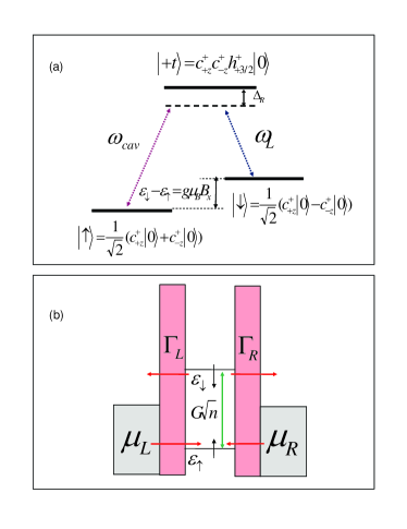
Figure 1: (a) Raman transition between the dot Zeeman states, $|\uparrow,\downarrow\rangle$, via an intermediate trion state, $|+t\rangle$, induced by a laser with frequency $\omega_{L}$ and a cavity mode with frequency $\omega_{cav}$. The spin eigenstates along the direction of the magnetic field are superpositions of spin eigenstates in the growth direction, $\hat{c}^{\dagger}_{\pm z}|0\rangle$. (b) Schematic of a single quantum dot indicating Zeeman energy levels in the dot and allowed tunnelling between leads and dot.

We assume that there are two electron reservoirs at chemical potential, $\mu_{L}=\mu_{R}=\mu$, that are coupled to the dots via tunnelling. We note, however, that our results are equally valid in the case of only a single reservoir. Only a single empty orbital energy level, $\varepsilon_{i}$, of the dot lies close to $\mu$. Here, the subscript $i$ denotes the particular dot. The Zeeman splitting between the two electron spin states is $\Delta_{i}=\varepsilon_{i,\downarrow}-\varepsilon_{i,\uparrow}=g^{(i)}_{x}\mu_{B}B$ where $B$ is a static magnetic field along the x-axis that is perpendicular to the growth direction (z). $\mu_{B}$ is the Bohr magneton and $g^{(i)}_{x}$ is the electronic g-factor of the $i^{th}$ dot along the direction of the magnetic field. The energy levels satisfy $\varepsilon_{i,\uparrow}=\varepsilon_{i}-\Delta_{i}/2<\mu<\varepsilon_{i,\downarrow}=\varepsilon_{i}+\Delta_{i}/2$ so that only spin up electrons can tunnel into the dot and only spin down electrons can tunnel out. In the limit of very large Coulomb blockade energy, only a single electron from the reservoir can occupy the dot resulting in the bare Hamiltonian for the dots and cavity field,

$$H_{0}=\hbar\omega_{cav}\hat{a}^{\dagger}\hat{a}+\sum_{i=1}^{N}\varepsilon_{i,\uparrow}\hat{c}^{\dagger}_{i,\uparrow}\hat{c}_{i,\uparrow}+\varepsilon_{i,\downarrow}\hat{c}^{\dagger}_{i,\downarrow}\hat{c}_{i,\downarrow}$$ (1)

where $\hat{c}_{{}_{i},\sigma}(\hat{c}^{\dagger}_{i,\sigma})$ are annihilation (creation) operators for electrons in dot $i$ with spin $\sigma$ in the x-direction of the magnetic field.

Transitions between the different electronic Zeeman states of a dot are induced via a two-photon Raman transition involving a strong laser field that may be treated classically and a quantized mode of the microcavity Djuric-Search-1 ; imamoglu . The two optical fields couple the electron spin states to a higher energy charged exciton state (trion) atature ; chen ; greilich ; dutt . The lowest energy trion states excited by $\sigma^{+}$ and $\sigma^{-}$ circularly polarized light are $|+t_{i}\rangle=\hat{c}^{\dagger}_{i,\uparrow}\hat{c}^{\dagger}_{i,\downarrow}\hat{h}^{\dagger}_{i,+3/2}|0\rangle$ and $|-t_{i}\rangle=\hat{c}^{\dagger}_{i,\uparrow}\hat{c}^{\dagger}_{i,\downarrow}\hat{h}^{\dagger}_{i,-3/2}|0\rangle$ , respectively. They consist of an electron singlet state and a heavy hole, where $\hat{h}^{\dagger}_{i,\pm 3/2}$ are heavy hole creation operators with spin projections $\pm\hbar 3/2$ along the z-axis and $|0\rangle$ is the empty dot state. The $\sigma^{+}$ polarized pump laser with frequency $\omega_{l}$ and Rabi frequency $\Omega_{l}$ couples each of the electron spin states to the $|+t_{i}\rangle$ trion state. Similarly, we assume that the cavity field, with vacuum Rabi frequency $g_{cav,i}$ for each dot and frequency $\omega_{cav}$, is also $\sigma^{+}$ polarized due to either the cavity construction or because it is driven by a $\sigma^{+}$ pump as discussed below note . When the two fields are far detuned from the creation energy for the $|+t_{i}\rangle$ state, the intermediate trion state can be adiabatically eliminated to give

$$H_{I}=i\hbar\sum_{i=1}^{N}g_{i}(\hat{a}\hat{c}^{\dagger}_{i,\downarrow}\hat{c}_{i,\uparrow}e^{i\omega_{l}t}-h.c.).$$ (2)

where $g_{i}=g_{cav,i}\Omega_{l}/4\Delta_{R}$ and $\Delta_{R}$ is the detuning from the trion state. In deriving Eq. 2, we have assumed that $|\Delta_{i}-(\omega_{cav}-\omega_{l})|\ll|\Delta_{i}+(\omega_{cav}-\omega_{l})|$ so that the non-resonant terms $\hat{a}^{\dagger}\hat{c}^{\dagger}_{i,\downarrow}\hat{c}_{i,\uparrow}e^{-i\omega_{l}t}+h.c.$ can be neglected. Since electrons enter the dot in the spin $\uparrow$ state, a photon must be absorbed from the cavity mode in order to generate a spin current. It is therefore necessary to pump the cavity field. We assume that the cavity is driven by a classical source oscillating at frequency $\omega_{p}$,

$$H_{P}=i\hbar\epsilon(\hat{a}^{\dagger}e^{-i\omega_{p}t}-h.c.),$$ (3)

which generates a coherent state in an empty cavity armen ; savage ; walls-milburn .

The explicit time dependence can be removed from $H_{I}$ and $H_{P}$ by transforming to a rotating frame for the field operators, $\hat{a}=\hat{A}e^{-i\omega_{p}t}$ and the dot operators, $\hat{c}_{i,\uparrow}=\hat{C}_{i,\uparrow}\exp(-i(\omega_{l}-\omega_{p})t/2)$ and $\hat{c}_{i,\downarrow}=\hat{C}_{i,\downarrow}\exp(i(\omega_{l}-\omega_{p})t/2)$. The Hamiltonian in the rotating frame is $H^{\prime}=H^{\prime}_{0}+H^{\prime}_{P}+H^{\prime}_{I}$,

$$H^{\prime}_{0} = \hbar(\omega_{cav}-\omega_{p})\hat{A}^{\dagger}\hat{A}+\sum_{i=1}^{N}\left(\varepsilon_{i}(\hat{C}^{\dagger}_{i,\uparrow}\hat{C}_{i,\uparrow}+\hat{C}^{\dagger}_{i,\downarrow}\hat{C}_{i,\downarrow})+(\Delta_{i}+\omega_{l}-\omega_{p})(\hat{C}^{\dagger}_{i,\downarrow}\hat{C}_{i,\downarrow}-\hat{C}^{\dagger}_{i,\uparrow}\hat{C}_{i,\uparrow})/2\right)$$ (4)

$$H^{\prime}_{I}+H^{\prime}_{P} = i\hbar\sum_{i=1}^{N}g_{i}(\hat{A}\hat{C}^{\dagger}_{i,\downarrow}\hat{C}_{i,\uparrow}-h.c.)+i\hbar\epsilon(\hat{A}^{\dagger}-h.c.)$$ (5)

From Eq. 4, one can clearly see that the resonance conditions are $\omega_{cav}=\omega_{p}$ and $\Delta_{i}=\omega_{p}-\omega_{l}$. We assume that former condition is always satisfied, while the latter condition cannot be satisfied for all dots due to variations in the magnetic moments between dots.

The dynamics of the system can be described in terms of the density operator, $\rho$ for the cavity plus dots. The master equation for $\rho$ is given by,

$$\dot{\rho}=-i[H^{\prime},\rho]-\Gamma_{cav}(\hat{A}^{\dagger}\hat{A}\rho-2\hat{A}\rho\hat{A}^{\dagger}+\rho\hat{A}^{\dagger}\hat{A})/2+\dot{\rho}|_{lead}$$ (6)

The first term describes coherent dynamics of the coupled QD-cavity system, the second term stands for the cavity decay walls-milburn , and the third term describes QD-lead coupling. Here we assume that the Coulomb blockade is so large that a second electron cannot tunnel into the dot if there is already one electron in the dot. The lead-dot coupling is most easily expressed in terms of the matrix elements of the density operator, $\rho^{(n,m)}_{\sigma_{i},\sigma^{\prime}_{i}}=\langle n,\sigma_{i}|\rho|\sigma^{\prime}_{i},m\rangle$ where $|\sigma_{i},n\rangle$ represents a state with $n$ photons in the cavity and $\sigma_{i}=0,\uparrow,\downarrow$ corresponding to no electrons, one spin up, or one spin down electron, respectively, on the $i^{th}$ dot. The specific form of the master equations for the lead coupling are dong ; Djuric-Search-1

$$\dot{\rho}^{(n,m)}_{0_{i},0_{i}}|_{lead} = \Gamma^{(-)}_{i}\rho^{(n,m)}_{\downarrow_{i},\downarrow_{i}}-\Gamma^{(+)}_{i}\rho^{(n,m)}_{0_{i},0_{i}}$$ (7)

$$\dot{\rho}^{(n,m)}_{\uparrow_{i},\uparrow_{i}}|_{lead} = \Gamma^{(+)}_{i}\rho_{0_{i},0_{i}}^{(n,m)}$$ (8)

$$\dot{\rho}^{(n,m)}_{\downarrow_{i},\downarrow_{i}}|_{lead} = -\Gamma^{(-)}_{i}\rho^{(n,m)}_{\downarrow_{i},\downarrow_{i}}$$ (9)

$$\dot{\rho}^{(n,m)}_{\uparrow_{i},\downarrow_{i}}|_{lead} = -\Gamma^{(-)}_{i}\rho^{(n,m)}_{\uparrow_{i},\downarrow_{i}}/2.$$ (10)

Here, $\Gamma_{i}^{(-)}=\Gamma^{(-)}_{i,L}+\Gamma^{(-)}_{i,R}$ is the rate at which spin down electrons tunnel out of the dots into the left and right leads and $\Gamma_{i}^{(+)}=\Gamma^{(+)}_{i,L}+\Gamma^{(+)}_{i,R}$ is the rate at which spin up electrons tunnel into the dots. (The subscripts $L$ and $R$ denote the tunnelling rates for the left and right leads, respectively.) We also assume that the coupling between the left and right leads and the dots are the same and that the tunnelling between the leads and the dot is spin independent, $\Gamma^{(+)}_{i,L}=\Gamma^{(-)}_{i,L}=\Gamma^{(+)}_{i,R}=\Gamma^{(-)}_{i,R}=\Gamma$. It is worth pointing out that because Eqs. 7-10 take into account large Coulomb blockade in the dots, they are slightly different from other master equations for dots that assume noninteracting electrons sun .

III Single Quantum Dot

First we consider the limit of a single quantum dot and exact two-photon resonance, $\Delta=\omega_{cav}-\omega_{l}$. We numerically solve for the steady state density matrix by first expressing the density matrix in vector form, $\rho^{(n,m)}_{\sigma_{i},\sigma^{\prime}_{i}}\rightarrow\vec{\rho}$, and rewriting Eq. 6 in matrix form,

$$d\vec{\rho}/dt=M\vec{\rho}$$ (11)

The steady state solution, $\vec{\rho}^{(0)}$, is given by the eigenvector of $M$ with zero eigenvalue djuric .

The steady state behavior of the system can be characterized by the Q-distribution for the intracavity optical fieldMeystre ; walls-milburn , $Q(\alpha)=\sum_{\sigma=0,\uparrow,\downarrow}\langle\alpha,\sigma|\rho^{(0)}|\alpha,\sigma\rangle/\pi$ where $|\alpha\rangle$ is a coherent state, $\hat{a}|\alpha\rangle=\alpha|\alpha\rangle$. The advantage of the Q-distribution is that it is positive semi-definite and can be used to make comparisons to classical phase space probability distributions. Figures 2 and 3 show $Q(\alpha)$ as well as the probability distribution for the photon number, $P(n)$. One can clearly see two peaks corresponding to the two stationary average cavity field amplitudes.

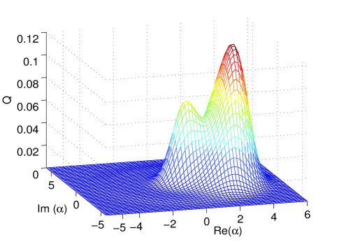
Figure 2: Q-distribution vs. $Re[\alpha]$ and $Im[\alpha]$ for $\Gamma_{cav}=0.2\Gamma$, $g=1.4\Gamma$ and $\epsilon=0.5\Gamma$.

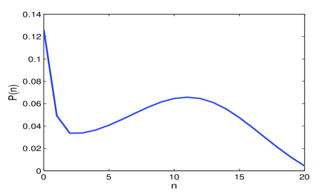
Figure 3: Photon probability distribution, $P(n)$, vs. cavity field photon number, $n$, for same parameters as Fig. 2, $\Gamma_{cav}=0.2\Gamma$, $g=1.4\Gamma$ and $\epsilon=0.5\Gamma$

The average spin current, $I_{s}=s(I_{\uparrow}-I_{\downarrow})$, is the same in the left and right leads with the stationary currents given by $\langle I_{\uparrow}\rangle=\Gamma\rho^{(0)}_{0,0}$ and $\langle I_{\downarrow}\rangle=-\Gamma\rho^{(0)}_{\downarrow,\downarrow}$. Here $\rho^{(0)}_{\sigma,\sigma}$ are the populations of the dot after tracing over the state of the cavity field. The average spin current can be expressed in terms of expectation values of the cavity field using Eq. 6,

$$\langle I_{S}\rangle=2s(2\epsilon Re[\langle\hat{a}\rangle]-\Gamma_{cav}\langle\hat{a}^{\dagger}\hat{a}\rangle)$$ (12)

Since the bimodality in $Q(\alpha)$ is in the amplitude, $|\alpha|$, both $Re[\hat{a}]$ and $\hat{a}^{\dagger}\hat{a}$ have two most probable values corresponding to the two peak locations, $\alpha_{j}$ for $j=1,2$. Consequently, individual measurements of the spin current would give results clustered around two most probable values

$$I_{S,j}=2s(2\epsilon Re[\alpha_{j}]-\Gamma_{cav}\alpha^{*}_{j}\alpha_{j}).$$ (13)

By contrast, the ensemble averaged spin current of Eq. 12 is $\langle I_{S}\rangle=Tr[I_{S}\rho^{(0)}]\approx P_{1}I_{S,1}+P_{2}I_{S,2}$ where $P_{j}$ are the total integrated probabilities for the two peaks in $Q(\alpha)$. Because of the large quantum fluctuations associated with a single dot, $\alpha^{(j)}$ are not truly stable points of the system. Instead, this system should behave in a similar manner to individual atoms in optical cavities, which exhibit stochastic jumps between the two stationary cavity field values induced by quantum noise armen ; savage ; Carmichael ; Mabuchi2 .

IV Semiclasical Bistability

Here we consider the equations of motion for the field and dot expectation values,

$$\alpha = \langle\hat{A}\rangle$$ (14)

$$s_{i} = \langle\hat{C}^{\dagger}_{i,\uparrow}\hat{C}_{i,\downarrow}\rangle$$ (15)

$$p_{i,\downarrow} = \langle\hat{C}_{i,\downarrow}^{\dagger}\hat{C}_{i,\downarrow}\rangle$$ (16)

$$p_{i,\uparrow} = \langle\hat{C}^{\dagger}_{i,\uparrow}\hat{C}_{i,\uparrow}\rangle,$$ (17)

which can be derived from Eq. 6 using $\langle\dot{O}\rangle=Tr[O\dot{\rho}]$. In order to have a finite system of equations, we must factorize the expectation values involving the cavity field and dots, $\langle\hat{A}^{\dagger}\hat{C}^{\dagger}_{i,\uparrow}\hat{C}_{i,\downarrow}\rangle\rightarrow\langle\hat{A}^{\dagger}\rangle\langle\hat{C}^{\dagger}_{i,\uparrow}\hat{C}_{i,\downarrow}\rangle=\alpha^{*}s_{i}$. The resulting equations are then,

$$\dot{p}_{i,\downarrow} = g_{i}(s_{i}\alpha^{*}+s_{i}^{*}\alpha)-\Gamma p_{i,\downarrow}$$ (18)

$$\dot{p}_{i,\uparrow} = -g_{i}(s_{i}\alpha^{*}+s_{i}^{*}\alpha)+\Gamma(1-p_{i,\downarrow}-p_{i,\uparrow})$$ (19)

$$\dot{\alpha} = -\sum_{i=1}^{N}g_{i}s_{i}-\Gamma_{cav}\alpha/2+\epsilon$$ (20)

$$\dot{s_{i}} = -i\delta_{i}s_{i}+g_{i}\alpha(p_{i,\uparrow}-p_{i,\downarrow})-\Gamma s_{i}/2$$ (21)

where $\delta_{i}=\Delta_{i}+\omega_{l}-\omega_{p}$. This ’semiclassical’ factorization ansatz amounts to neglecting quantum mechanical correlations between the cavity field and dots and is usually assumed to be valid in the limit of large ‘classical’ systemsarmen . Experiments with atoms in optical cavities in the strong coupling regime showed good agreement with such a semiclassical theory for $N>15$ atoms except for very close to the end points of the bistable regionrempe . We therefore restrict our treatment to $N\gg 1$ dots.

In order to derive analytic expressions, we will first neglect inhomogeneous broadening, $\delta_{i}=0$, and variations of the vacuum Rabi frequency due to random positions of the dots relative to the cavity mode, $g_{i}=g_{0}$. We will account for these effects later by numerical averaging over $\delta_{i}$ and $g_{i}$. We then define new variables for the total population and polarization, $P_{\sigma}=\sum_{i}p_{i,\sigma}$ and $S=\sum_{i}s_{i}$. By introducing the polar representation, $S=|S|e^{i\theta}$, $\alpha=|\alpha|e^{i\varphi}$ and $\epsilon=|\epsilon|e^{i\phi}$, and using the positive definiteness of $P_{\sigma}$, one sees that the phases are locked, $\varphi=\phi=\theta$.

The differential equations for $|\alpha|$, $|S|$, and $P_{\sigma}$ have steady state solutions given by

$$12g_{0}^{2}\Gamma_{cav}|\alpha|_{j}^{3} - 24g_{0}^{2}|\epsilon||\alpha|_{j}^{2}+(4g_{0}^{2}\Gamma N+\Gamma^{2}\Gamma_{cav})|\alpha|_{j}$$ (22)

$$- 2\Gamma^{2}|\epsilon|=0$$

$$|S|_{j} = \frac{2|\epsilon|-\Gamma_{cav}|\alpha|_{j}}{2g_{0}}$$ (23)

$$P_{\downarrow j} = \frac{-\Gamma_{cav}|\alpha|_{j}^{2}+2|\epsilon||\alpha|_{j}}{\Gamma}$$ (24)

$$P_{\uparrow j} = N-2P_{\downarrow j}.$$ (25)

Here, $|\alpha|_{j}$ for $j=1,2,3$, are the roots of Eq.  22 and the steady spin current is given by $I_{sj}=2s\Gamma P_{\downarrow j}$

In the limit of negligibly small cavity decay, $\Gamma_{cav}\ll|\epsilon|$, $\Gamma$, $g_{0}$, Eq.  (22) becomes quadratic with the two stationary solutions,

$$|\alpha|_{1,2}=\frac{\Gamma N}{12|\epsilon|}\left(1\pm\sqrt{1-\frac{12|\epsilon|^{2}}{N^{2}g_{0}^{2}}}\right)$$ (26)

for $0<12|\epsilon|^{2}/N^{2}g_{0}^{2}<1$. By contrast, in the limit $\Gamma\rightarrow 0$, the only nonzero solution for the cavity field is $|\alpha|=2|\epsilon|/\Gamma_{cav}$. This limit is different from the case of atomic OB where bistability in the phase of $\alpha$ exists in the limit that the spontaneous emission rate goes to zero Mabuchi2 ; Carmichael . The difference arises from the fact that $\Gamma$ represents both the pumping rate and the decay rate for electrons in the dots. When $\Gamma=0$, electrons cannot tunnel into the dots and interact with the cavity, which effectively decouples the dots from the cavity field.

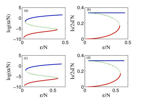
Figure 4: (a,c) Cavity field amplitude $\log_{10}(|\alpha|/N)$ vs. $|\epsilon|/N$.(b, d) Spin current, $I_{S}/2s\Gamma N$ vs. $|\epsilon|/N$. For (a) and (b), $g_{0}=1.4\Gamma$ and $\Gamma_{cav}=0.2\Gamma$. For (c) and (d), $g_{0}=2.0\Gamma$, $\Gamma_{cav}=0.5\Gamma$. In all cases the number of dots is $N=50$ and $|\epsilon|/N$ is plotted in units of $\Gamma$.

Solutions of Eq. 22 are presented in Fig. 4 as a function of the driving field, $\epsilon$. Three positive real solutions of Eq. 22 exist for $\epsilon$ in the interval $|\epsilon|_{1}<|\epsilon|<|\epsilon|_{2}$, where

$$|\epsilon|_{1,2}=\frac{g_{0}N}{2\sqrt{6}}\sqrt{1+\frac{5}{2}\frac{N_{0}}{N}-\frac{1}{8}\left(\frac{N_{0}}{N}\right)^{2}\mp\left(1-\frac{N_{0}}{N}\right)^{3/2}}$$ (27)

where $N_{0}=2\Gamma\Gamma_{cav}/g_{0}^{2}$ is the critical dot number. By analogy to atomic cavity QED, it is the number of dots necessary to significantly modify the resonant properties of the cavity armen . The requirement that $(1-N_{0}/N)^{3/2}$ be real implies that $N_{0}<N$, which reduces to the requirement of strong coupling to the cavity when $N=1$, as one would expect. Eq. 27 corresponds to the range of $|\epsilon|$ for which bistability occurs. One can clearly see from Fig. 4 that the bistability of $\alpha$ also leads to bistability and hysteresis for the spin current. We have analyzed the stability of the three steady state solutions as outlined in the appendix and determined that the two positive slope solutions in Fig. 4 (represented by the solid lines) are stable while the negative slope solutions (dotted lines) are unstable. For the cavity field, the lower stable branch corresponds to a nearly empty cavity, $\alpha\approx 0$ but with a finite increasing spin current, $I_{S}\approx 0$ up to $I_{S}\approx 2sN\Gamma\times 0.2$. Since $g_{0},\Gamma>\Gamma_{cav}$, this solution corresponds to a photon entering the cavity and being almost instantaneously absorbed by a dot, which then leads to the creation of one unit of spin current. The upper stable branch corresponds to a large cavity field, $\alpha\approx 0.1N$ up to $\alpha\approx 10N$, with a constant spin current of $I_{S}=2s\Gamma N/3$. This value of the spin current corresponds to a saturated transition in the dot with equal probabilities for the two spin states along with the empty dot state, $\rho^{(0)}_{0_{i},0_{i}}=\rho^{(0)}_{\uparrow_{i},\uparrow_{i}}=\rho^{(0)}_{\downarrow_{i},\downarrow_{i}}=1/3$. In this case, a spin current per dot of $2s\Gamma/3$ was previously found to be the maximum spin current that could be generated by a single dot using a classical field dong .

In order to account for variations in $\delta_{i}$ and $g_{i}$ as a result of the random sizes and positions of the dots during the growth process, we assume that the variations can be modelled using Gaussian probability distributions,

$$P_{d}(\delta_{i}) = \frac{1}{\sigma_{d}\sqrt{2\pi}}e^{-\delta_{i}^{2}/2\sigma_{d}^{2}}$$ (28)

$$P_{g}(g_{i}) = \frac{1}{\sigma_{g}\sqrt{2\pi}}e^{-(g_{i}-g_{0})^{2}/2\sigma_{g}^{2}}.$$ (29)

The contribution of each of the dots to the cavity field appears as a summation over the dot polarizations in Eq. 20, which must now be replaced with an integration over the probability distributions, $\sum_{i}g_{i}s_{i}\rightarrow N\int\int d\delta_{i}dg_{i}P_{d}(\delta_{i})P_{g}(g_{i})g_{i}s_{i}$. The resulting equation for the steady state cavity field is then

$$|\epsilon|-\Gamma_{cav}|\alpha|/2 = N\int d\delta_{i}dg_{i}P_{d}(\delta_{i})P_{g}(g_{i})f(\delta_{i},g_{i})$$ (30)

$$f(\delta_{i},g_{i}) = \frac{g_{i}^{2}|\alpha|\Gamma}{6g_{i}^{2}|\alpha|^{2}+\Gamma^{2}/2+2\delta_{i}^{2}}.$$ (31)

The cavity field amplitude can then be used to calculate the spin current using $I_{s}=2s\Gamma\sum_{i}p_{i,\downarrow}=2s(2|\alpha||\epsilon|-\Gamma_{cav}|\alpha|^{2})$. Note that in deriving Eq. 30 we have made use of the fact that the sine of the phase difference between the cavity and driving fields, $\sin(\phi-\varphi)$, vanishes when averaged over a probability distribution that is even about $\delta_{i}=0$. One can see from Eq. 30-31, that for small cavity fields $g_{i}|\alpha|\ll\Gamma$, the homogenous broadening of the dot levels due to the leads dominates over the inhomogeneous broadening of the dot levels when $\sigma_{d}\ll\Gamma$. On the other hand for large cavity fields, $g_{i}|\alpha|\gg\Gamma,\sigma_{d}$, power broadening dominates over homogeneous and inhomogeneous broadening of the dot levels and the cavity field is independent of $\sigma_{d}$.

Figures 5 and 6 show the cavity field amplitude and spin current as a function of the driving field amplitude, $\epsilon$, for different $\sigma_{d}$ and $\sigma_{g}$. For the Rabi frequencies, $\sigma_{g}$ was chosen to be $20\%$ or $40\%$ of the mean while for the Zeeman splitting we chose $\sigma_{d}>\Gamma$ for all curves. One can see that for increasing $\sigma_{d}$ and $\sigma_{g}$ the range of $\epsilon$ where bistability occurs is reduced. This can be understood as the result of fewer dots that are both resonant with the cavity mode and strongly coupled to it.

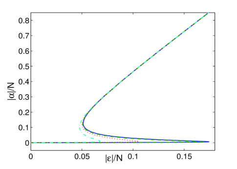
Figure 5: Cavity field amplitude, $|\alpha|/N$, vs. $|\epsilon|/N$ in units of $\Gamma$ for $N=50$ dots, $g_{0}=1.6\Gamma$, and $\Gamma_{cav}=0.4\Gamma$. The different curves correspond to: $\sigma_{d}=2\Gamma$ and $\sigma_{g}=0.2g_{0}$ (solid line); $\sigma_{d}=2\Gamma$ and $\sigma_{g}=0.4g_{0}$ (dashed line); $\sigma_{d}=4\Gamma$ and $\sigma_{g}=0.2g_{0}$ (dotted line); $\sigma_{d}=7\Gamma$ and $\sigma_{g}=0.2g_{0}$ (dashed dot line).

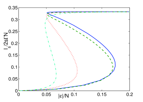
Figure 6: Spin current, $I_{s}/2s\Gamma N$, vs. $|\epsilon|/N$ in units of $\Gamma$ for the same parameters as Fig. 5: $N=50$ dots and $g_{0}=1.6\Gamma$, $\Gamma_{cav}=0.4\Gamma$. The different curves correspond to: $\sigma_{d}=2\Gamma$ and $\sigma_{g}=0.2g_{0}$ (solid line); $\sigma_{d}=2\Gamma$ and $\sigma_{g}=0.4g_{0}$ (dashed line); $\sigma_{d}=4\Gamma$ and $\sigma_{g}=0.2g_{0}$ (dotted line); $\sigma_{d}=7\Gamma$ and $\sigma_{g}=0.2g_{0}$ (dashed dot line).

V Conclusion

In conclusion, we have studied the generation of spin currents by electrical transport through quantum dots coupled to a single mode of an optical microcavity. We have shown that when the cavity field is coherently driven, absorptive optical bistability occurs in the cavity field. Since the steady state spin current is proportional to both the cavity field amplitude and number of photons in the cavity, OB necessarily leads to bistability in the spin current. Moreover, we have shown that this bistability persists in the presence of inhomogeneous broadening of the dots’ Zeeman splitting and vacuum Rabi frequencies.

The cavity field and spin current could be made to switch between the two stable states by varying the driving field amplitude, $\epsilon$, beyond the endpoints of the bistable regionMeystre . One might then envision using this system as an optically controlled spin current switch, which could be used, for example, to transfer optically encoded digital information into a spin current. In a future publication we plan to explore quantum noise induced switching between stationary spin currents states for the single quantum dot case using a stochastic master equation Mabuchi2 .

VI Appendix: Linear Stability Analysis

In order to analyze the stability of the steady state solutions, we consider small fluctuations $\delta P_{\downarrow}$, $\delta P_{\uparrow}$, $\delta\alpha$ and $\delta s$ about steady the state solutions of Eqs. 18-21,

$$P_{\downarrow}(t) = P_{\downarrow}^{(0)}+\delta P_{\downarrow}(t)$$ (32)

$$P_{\uparrow}(t) = P_{\uparrow}^{(0)}+\delta P_{\uparrow}(t)$$ (33)

$$\alpha(t) = \alpha^{(0)}+\delta\alpha(t)$$ (34)

$$s(t) = s^{(0)}+\delta s(t).$$ (35)

where $P_{\downarrow}^{(0)}$, $P_{\uparrow}^{(0)}$, $\alpha^{(0)}$ and $s^{(0)}$ correspond to one of the three steady solutions solutions given by Eq. 22. By inserting Eqs. 32-35 into Eqs. 18-21 and discarding terms that are quadratic in the fluctuations, we obtain the following linear equations for the fluctuations,

$$\frac{d}{dt}\left(\begin{array}[]{c}\delta P_{\downarrow}\\ \delta P_{\uparrow}\\ \delta\alpha\\ \delta\alpha^{*}\\ \delta s\\ \delta s^{*}\\ \end{array}\right)=\left(\begin{array}[]{cccccc}-\Gamma&-\Gamma&gs^{*(0)}&gs^{(0)}&g\alpha^{*(0)}&g\alpha^{(0)}\\ 0&-\Gamma&-gs^{*(0)}&-gs^{(0)}&-g\alpha^{*(0)}&-g\alpha^{(0)}\\ 0&0&-\frac{\Gamma_{cav}}{2}&0&g&0\\ 0&0&0&-\frac{\Gamma_{cav}}{2}&0&g\\ -g\alpha^{(0)}&g\alpha^{(0)}&g(P_{\uparrow}^{(0)}-P_{\downarrow}^{(0)})&0&-\frac{\Gamma}{2}&0\\ -g\alpha^{*(0)}&g\alpha^{*(0)}&0&g(P_{\uparrow}^{(0)}-P_{\downarrow}^{(0)})&0&-\frac{\Gamma}{2}\\ \end{array}\right)\left(\begin{array}[]{c}\delta P_{\downarrow}\\ \delta P_{\uparrow}\\ \delta\alpha\\ \delta\alpha^{*}\\ \delta s\\ \delta s^{*}\\ \end{array}\right)={\bf J}\left(\begin{array}[]{c}\delta P_{\downarrow}\\ \delta P_{\uparrow}\\ \delta\alpha\\ \delta\alpha^{*}\\ \delta s\\ \delta s^{*}\\ \end{array}\right)$$ (36)

The associated characteristic equation for the eigenvalues of ${\bf J}$ is a sixth order polynomial

$$\sum_{i=1}^{6}a_{l}\lambda^{l}=0$$ (37)

A particular steady state solution, $\{P_{\downarrow}^{(0)},P_{\uparrow}^{(0)},\alpha^{(0)},s^{(0)}\}$, is stable if $Re[\lambda]<0$ for all six of the eigenvalues since any small noise induced fluctuation will then decay away exponentially. Steady state solutions with at least one eigenvalue satisfying $Re[\lambda]>0$ are unstable since small fluctuations will grow exponentially with time. Numerical solutions for the eigenvalues for each of the three steady states in Figs. 4-6 indicate that two of the roots are stable and one is unstable. The stable roots correspond to the upper and lower branches in Figs. 4-6 that have positive slope while the middle branch with negative slope is unstable.

References

- (1) P. Meystre and M. Sargent III, Elements of Quantum Optics, Springer.
- (2) A. Szöke , V. Danue , J. Goldhar, and N. A. Kurnit , Appl. Phys. Lett. 15 376 (1969).
- (3) H. M. Gibbs, S. L. McCall and T. N. C. Venkatesan, Phys. Rev. Lett. 36, 1135 (976).
- (4) A. Miller , D. A. B. Miller and S. D. Smith, Adv. Phys. 30 697 (1981)’
- (5) E. Abraham, and S. D. Smith, Rep. Prog. Phys. 45, 815 (1982).
- (6) H. M. Gibbs, Optical Bistability: Controlling Light with Light (academic, New York) (1885).
- (7) P. Mandel, S. D. Smith, and B. S. Wherrett, From Optical Bistability towards Optical Computing (North-Holland, Amsterdam) (1987).
- (8) M. Warren, S. W. Koch, and H. M. Gibbs, IEEE Comput. Sci. Eng. 20, 68 (1987).
- (9) E. Abraham and S. D. Smith, Rep. Prog. Phys. 45, 815 (1981).
- (10) R. Bonifacio and L. A. Lugiato ,Opt. Commun. 19, 172 (1976).
- (11) Igor Zutic, Jaroslav Fabian, S. Das Darma, Rev. Mod. Phys. 76, 323 (2004).
- (12) M. A. M. Gijs and G. E. W. Bauer, Adv. Phys. 46, 285 (1997).
- (13) M. I. D’yakonov and V. I. Perel’, JETP Lett. 13, 467 (1971); J. E. Hirsch, Phys. Rev. Lett. 83, 1834 (1999); S. Zhang, Phys. Rev. Lett. 85, 393 (2000); T. P. Pareek, Phys. Rev. Lett. 92, 076601 (2004).
- (14) E. I. Rashba, Physica E (Amsterdam) 20, 189 (2004).
- (15) Martin J. Stevens, Arthur L. Smirl, R. D. R. Bhat, Ali Najmaie, J. E. Sipe, and H. M. van Driel, Phys. Rev. Lett. 90, 136603 (2003); R. D. R. Bhat and J. E. Sipe, Phys. Rev. Lett. 85, 5432 (2000).
- (16) A. Najmaie, E. Ya. Sherman, J. E. Sipe, Phys. Rev. Lett. 95, 056601 (2005).
- (17) E. R. Mucciolo, C. Chamon, and C. M. Marcus, Phys. Rev. Lett. 89, 146802 (2002).
- (18) Susan K. Watson, R. M. Potok, and C. M. Marcus, and V. Umansky, Phys. Rev. Lett. 91, 258301 (2003).
- (19) P. Sharma and C. Chamon, Phys. Rev. Lett. 87, 096401 (2001); R. Citro, N. Andrei, Q. Niu, Phys. Rev. B 68, 165312 (2003).
- (20) R. Benjamin and C. Benjamin, Phys. Rev. B 69, 085318 (2004).
- (21) M. Blaauboer and C. M. L. Fricot, Phys. Rev. B 71, 041303(R).
- (22) E. Sela and Y. Oreg, Phys. Rev. B 71, 075322 (2005).
- (23) B. G. Wang, J. Wang, and Hong Guo, Phys. Rev. B 67, 92408 (2003); P. Zhang, Qi-Kun Xue, and X. C. Xie, Phys. Rev. Lett. 91, 196602 (2003).
- (24) Bing Dong, H. L. Cui, and X. L. Lei, Phys. Rev. Lett. 94, 066601 (2005).
- (25) Ivana Djuric and Chris P. Search, Phys. Rev. B 74, 115327 (2006).
- (26) M. A. Armen and H. Mabuchi, Phys. Rev. A 73, 063801 (2006).
- (27) M. Gurioli, L. Cavigli, G. Khitrova, and H. Gibbs, Phy. Stat. Sol. (a) 201, 661 (2004); M. Gurioli, L. Cavigli, G. Khitrova, and H. Gibbs, Semicond. Sci. Technol. 19, S345 (2004).
- (28) J. P. Reithmaier, G. Sȩk, A. Löffler, C. Hofmann, S. Kuhn, S. Reitzenstein, L. V. Keldysh, V. D. Kulakovskii, T. L. Reinecke and A. Forchel, Nature 432, 197 (2004); T. Yoshie, A. Scherer, J. Hendrickson, G. Khitrova, H. M. Gibbs, G. Rupper, C. Ell, O. B. Shchekin, and D. G. Deppe, Nature 432, 200 (2004).
- (29) E. Peter, P. Senellart, D. Martrou, A. Lemaître, J. Hours, J. M. Gérard, and J. Bloch, Phys. Rev. Lett. 95, 067401 (2005).
- (30) K. H. Schmidt, M. Versen, U. Kunze, D. Reuter, and A. D. Wieck, Phys. Rev. B 62, 15879 (2000).
- (31) T. Ota, K. Ono, M. Stopa, T. Hatano, S. Tarucha, H. Z. Song, Y. Nakata, T. Miyazawa, T. Ohshima, and N. Yokoyama, Phys. Rev. Lett. 93, 066801 (2004).
- (32) P. Barthold, F. Hohls, N. Maire, K. Pierz, and R. J. Haug, Phys. Rev. Lett. 96, 246804 (2006).
- (33) G. Kieblich, A. Wacker, and E. Scholl, S. A. Vitusevich, A. E. Belyaev, S. V. Danylyuk, A. Forster, N. Klein, and M. Henini, Phys. Rev. B 68, 125331 (2003).
- (34) D. Heis, M. Kroutvar, J. J. Finley, and G. Abstreiter, Solid State Communications 135, 591 (2005).
- (35) Mete Atatüre, Jan Dreiser, Antonio Badolato, Alexander Högele, Khaled Karrai, and Atac Imamoglu, Science 312, 551 (2006).
- (36) A. Imamoḡlu, D. D. Awschalom, G. Burkard, D. P. DiVincenzo, D. Loss, M. Sherwin, and A. Small, Phys. Rev. Lett. 83, 4204 (1999).
- (37) Pochung Chen, C. Piermarocchi, L. J. Sham, D. Gammon, D. G. Steel, Phys. Rev. B 69, 075320 (2004).
- (38) A. Greilich, R. Oulton, E. A. Zhukov, I. A. Yugova, D. R. Yakovlev, M. Bayer, A. Shabaev, Al. L. Efros, I. A. Merkulov, V. Stavarache, D. Reuter, and A. Wieck, Phys. Rev. Lett. 96, 227401 (2006).
- (39) M. V. Gurudev Dutt, Jun Cheng, Bo Li, Xiaodong Xu, Xiaoqin Li, P. R. Berman, D. G. Steel, A. S. Bracker, D. Gammon, Sophia E. Economou, Ren-Bao Liu, and L. J. Sham, Phys. Rev. Lett. 94, 227403 (2005).
- (40) A linearly polarized cavity will also suffice. However it will also couple the Zeeman states to the trion state leading to additional AC stark shifts.
- (41) C. M. Savage and H. J. Carmichael, IEEE J. Quantum Electronics 24, 1495 (1988).
- (42) D. F. Walls and G. J. Milburn, Quantum Optics (Springer-Verlab, Berlin, 1994).
- (43) He Bi Sun and G. J. Milburn, Phys. Rev. B 59 10748 (1999).
- (44) Ivana Djuric, Bing Dong, and H.L. Cui, J. Appl. Phys. 99, 063710 (2006).
- (45) P. Alsing and H. J. Carmichael, Quantum Opt. 3 13 (1991).
- (46) H. Mabuchi and H. M. Wiseman, Phys. Rev. Lett. 81, 4620 (1998).
- (47) G. Rempe, R. J. Thompson, R. J. Brecha, W. D. Lee, and H. J. Kimble, Phys. Rev. Lett. 67, 1727 (1991).