Gap solitons in Bose-Einstein condensates in linear and nonlinear optical lattices

Abstract

Properties of localized states on array of BEC confined to a potential, representing superposition of linear and nonlinear optical lattices are investigated. For a shallow lattice case the coupled mode system has been derived. The modulational instability of nonlinear plane waves is analyzed. We revealed new types of gap solitons and studied their stability. For the first time a moving soliton solution has been found. Analytical predictions are confirmed by numerical simulations of the Gross-Pitaevskii equation with jointly acting linear and nonlinear periodic potentials.

I Introduction

The Bose-Einstein condensate in a linear periodic potential attracts a great attention for last years. Many fascinating phenomena like Josephson oscillations, macroscopic quantum tunnelling and localization, gap solitons etc have been predicted and observed in the experiments Morsh ; BK . The description of these phenomena is based on the Gross-Pitaevskii equation governing the condensate wave function and having terms corresponding to the external linear (varying in space and time) potential and a mean field nonlinearity(taking into account many body effects). The strength of the mean field nonlinearity is proportional to the atomic scattering length. We can imagine the BEC system, when the strength of two body interaction is varying in spaceAS03 ; kevrekidis ; AGKT ; GA . For a periodic variation of scattering length it leads to appearance of a nonlinear periodic potential. The ground state and dynamics of localized states of BEC under action of the nonlinear periodic potential have been studied recently in papers SM ; AG ; Fibich .

Periodic potential in BECOFR1 ; OFR2 can be generated by optical methods. Two types of optical lattices are considered: a linear periodic potential induced by the standing laser field Morsh and a nonlinear optical lattice produced by two counter propagating laser beams with parameters near the optically induced Feshbach resonance (FR) SM ; AG . Periodic variation of the laser field intensity in space by proper choice of the resonance detuning can lead to the spatial dependence of the scattering length OFR2 . Then the nonlinear term in the GP equation becomes periodically modulated in space, leading to the generation of nonlinear optical lattice.

In real physical situations exact resonance condition is not attained and the potential represents the mixture of linear and nonlinear optical lattices. This type of periodic potential also can be produced by two pairs of counter propagating laser beams, when one pair produces linear optical lattice, and second pair - a nonlinear one. Another interesting system where the superposition of linear and nonlinear periodic potentials can be realized is the array of fermion-boson mixturesKonotop06 . Gap solitons(GS) in a photorefractive crystal, considered recently in Malomed05 , also originate from the jointly acting linear and nonlinear periodic potentials. But the last system is different from ones considered here, since its nonlinearity has saturable nature.

Two types of optical lattices can be distinguished: a shallow and a deep. The first type is realized for $V<E_{R}$, and the second one for $V>5E_{R}$, where $V$ is the strength of the periodic potential and $E_{R}=\hbar^{2}k^{2}/2m$ is the recoil energy, $k$ is the laser beam wavenumber.

In the case of a shallow optical lattice (that will be considered in this work) we can apply a coupled mode approach. The coupled-mode theory describes general properties of gap solitons, taking into account interaction of counter propagating waves. Analytical solutions have been found for the case of the Kerr nonlinearity in AW . In our case the system of coupled-mode theory has more complicated character and is analogous to the studied in the nonlinear optics for a deep Bragg grating caseIizuka and a nonlinear layered structuresPel1 . In the case of vanishing nonlinear lattice a periodic potential transforms into the standard linear one Sterke ; YS ; EC . We study the modulational instability(MI) of nonlinear plane waves which is important mechanism for the soliton and solitonic pattern generation. The gap soliton solutions of this modified coupled mode system are obtained and their stability is analyzed.

The emphasis is also given to the travelling gap soliton (GS) solutions. We obtain solutions for moving GS and study collisions between solitons having an inelastic character. In optics they have been experimentally observed in fibers with Bragg gratingEggleton . It will be interesting to observe the travelling GS in BEC with linear and nonlinear optical lattices.

The case of deep optical lattice can be investigated in the framework of the tight-binding approximation. The GP equation then transforms into the modified discrete nonlinear Schrödinger equation (NLSE) with a nonlocal nonlinearityTS ; ABDKS ; Khare . Analysis of MI and the discrete breathers for this model requires separate investigation.

The paper is organized as follows. In Section II we describe the model and derive the coupled mode system. In Section III modulational instability of cw solutions is investigated. The gap soliton solutions and their stability is discussed in Section IV. The moving gap soliton solutions and the solitons collision are studied in Section V. Main results of the paper are summarized in Section VI.

II The model. Coupled-mode equations

We consider here the dynamics of BEC under jointly acting linear and nonlinear optical lattices. First type of potential is induced by a periodic interference pattern from the counter propagating laser beamsMorsh . Second type of potential is produced by the optically induced Feshbach resonance OFR2 . According to this technique, periodic variation of laser field intensity in the standing wave $I(x)=I_{0}\cos^{2}(kx)$ produces periodic variation of the atomic scattering length $a_{s}$, i.e.

$$a_{s}=a_{s0}+\alpha\frac{I(x)}{\delta+\alpha I},$$ (1)

where $\delta$ is the detuning. At large detunings from FR $a_{s}=a_{s0}+a_{s1}\cos^{2}(kx)$.

In the recent experiment with the ⁸⁷Rb condensate the scattering length has been optically manipulatedOFR1 . The number of of atoms was $10^{6}$ and laser power was approximately $500W/cm^{2}$. By choice of the laser power and detuning of the laser beam around the photo-association resonance the scattering length was changed over one order of magnitude, from $10a_{0}$ to $190a_{0}$ ($a_{0}$ is the Bohr radius).

The quasi 1D GP equation for the BEC wavefunction under action of superposition of a linear and nonlinear optical lattice is SM ; AG :

$$i\hbar\psi_{T}=-\frac{\hbar^{2}}{2m}\psi_{XX}+V_{0}\cos^{2}(kx)\psi+(g_{1D}^{(0)}$$

$$+g_{1D}^{(1)}\cos^{2}(kx))|\psi|^{2}\psi,$$ (2)

where $g_{1D}^{(0,1)}=2\hbar a_{s0,1}\omega_{\perp}$, and $a_{s}$ is the atomic scattering length. Introducing dimensionless variables

$$\epsilon=\frac{V_{0}}{2E_{R}},\ E_{R}=\frac{\hbar^{2}k^{2}}{2m},\ x=Xk,\ t=\frac{T}{T_{0}},$$

$$T_{0}=\frac{E_{R}}{\hbar},\ u=\sqrt{\frac{2|a_{s0}|\omega_{\perp}}{E_{R}}}\psi e^{-i\epsilon t},\ \kappa=\frac{a_{s1}}{a_{s0}}.$$

we can rewrite the equation in the form

$$iu_{t}+u_{xx}+(\gamma_{0}+\kappa\cos(2x))|u|^{2}u-\epsilon\cos(2x)u=0.$$ (3)

$\gamma_{0}>0$ corresponds to the attractive and $\gamma_{0}<0$ - to the repulsive condensates respectively. We will consider the shallow lattice case, when $\epsilon\ll 1$. In this case one can derive the system of coupled mode equations. Let us represent the field $u(x,t)$ in the form

$$u(x,t)=(A(x,t)e^{ix}+B(x,t)e^{-ix})e^{-it}.$$ (4)

Collecting terms at $e^{\pm ix}$ we obtain the system of coupled mode equations

$$iA_{t}+2iA_{x}+\gamma_{0}(|A|^{2}A+2|B|^{2}A)$$

$$-\frac{\epsilon}{2}B+\frac{\kappa}{2}(|B|^{2}B+2|A|^{2}B+A^{2}B^{\ast})=0,$$ (5)

$$iB_{t}-2iB_{x}+\gamma_{0}(|B|^{2}B+2|A|^{2}B)$$

$$-\frac{\epsilon}{2}A+\frac{\kappa}{2}(|A|^{2}A+2|B|^{2}A+B^{2}A^{\ast})=0.$$ (6)

In comparison with the standard coupled-mode system, this system includes terms corresponding to the nonlinear coupling $\sim\kappa$.

Note that at small amplitudes of waves $A,B\sim\exp(ikx-i\omega t)$ the dispersion law is $\omega^{2}=\epsilon^{2}/4+k^{2}$, and this system has the forbidden gap for $-\epsilon/2<\omega<\epsilon/2$. The system is unchanged if we perform transformations $\gamma_{0}\rightarrow-\gamma_{0},\ \kappa\rightarrow\kappa,\ \ (A,B,\omega)\rightarrow(A^{\ast},-B^{\ast},-\omega)$.

It means that results obtained for the first excited band $\omega>\epsilon/2$ with repulsive interactions can be valid for the zero order allowed band $\omega<-\epsilon/2$ with attractive interactionsYS .

The Eqs. (II), (II) read as

$$iA(B)_{t}=\frac{\delta H}{\delta A^{\ast}(B^{\ast})}.$$

The Hamiltonian $H$ has the following form

$$H=\int dx[\frac{i}{2}(A^{\ast}A_{x}-AA^{\ast}_{x}-B^{\ast}B_{x}+BB^{\ast}_{x})-$$

$$\frac{\epsilon}{2}(BA^{\ast}+AB^{\ast})+\frac{\gamma_{0}}{2}(4|A|^{2}|B|^{2}+$$

$$|A|^{4}+|B|^{4})+\frac{\kappa}{2}(|A|^{2}+|B|^{2})(BA^{\ast}+B^{\ast}A)].$$ (7)

The number of atoms is conserved

$$N=\int_{-\infty}^{\infty}dx[|A|^{2}+|B|^{2}].$$ (8)

III Modulational instability

We start with consideration of the modulational instability(MI) phenomena in this model. The MI is a general phenomenon originating from the interplay between nonlinearity and dispersion and it consists in the instability of nonlinear plane wave solutions against long wavelength modulations. In periodic media the periodicity leads to modification of the dispersion law. MI is known to be an important mechanism for the generation of solitons and solitonic trains in nonlinear optics and Bose-Einstein condensates Sterke2 ; ADG ; KS . The MI in photonic crystals with a deep Bragg grating recently has been investigated numerically in Ref.Porz . The cw solutions of the coupled-mode system are sought using the parametrization suggested in Sterke2

$$A=\frac{\alpha}{\sqrt{1+f^{2}}}e^{i(Qx-\Omega t)},\ B=\frac{\alpha f}{\sqrt{1+f^{2}}}e^{i(Qx-\Omega t)},$$ (9)

where $\alpha^{2}=|A|^{2}+|B|^{2}$ and we have

$$\Omega = -\frac{3\gamma_{0}}{2}\alpha^{2}-\frac{\epsilon}{4}\frac{1+f^{2}}{f}-\frac{\kappa\alpha^{2}}{4}\frac{1+6f^{2}+f^{4}}{f(1+f^{2})},$$ (10)

$$Q = -\frac{\gamma_{0}\alpha^{2}}{4}\frac{1-f^{2}}{1+f^{2}}+\frac{\epsilon}{8}\frac{1-f^{2}}{f}-\frac{\kappa\alpha^{2}}{8}\frac{1-f^{2}}{f}.$$ (11)

When $\kappa=0$ the result for a standard coupled-mode system is reproduced. The physical mean of the parameter $f$: $f<0$ corresponds to the top of a band gap of the linear dispersion curve, and $f>0$ to the bottom of a band gap .

To study MI we look for the solution of the form

$$A=\left(\frac{\alpha}{\sqrt{1+f^{2}}}+\delta A(x,t)\right)e^{i(Qx-\Omega t)},$$

$$B=\left(\frac{\alpha f}{\sqrt{1+f^{2}}}+\delta B(x,t)\right)e^{i(Qx-\Omega t)},$$ (12)

where $\delta A$ and $\delta B$ are perturbations of the cw solution. Substituting these expressions into Eqs.(II) and using a linear approximation, we get the system for $\delta A(x,t),\delta B(x,t)$

$$i\delta A_{t}+2i\delta A_{x}+\frac{\epsilon}{2}f\delta A-\frac{\epsilon}{2}\delta B+$$

$$G[\delta A+\delta A^{\ast}+2f(\delta B+\delta B^{\ast})]+$$

$$K\left[\delta B^{\ast}+2\delta B+\frac{f(1-f^{2})}{1+f^{2}}\delta A+\frac{2f}{1+f^{2}}\delta A^{\ast}\right]=0,$$

$$i\delta B_{t}-2i\delta B_{x}+\frac{\epsilon}{2f}\delta B-\frac{\epsilon}{2}\delta A+$$

$$G[f^{2}(\delta B^{\ast}+\delta B)+2f(\delta A+\delta A^{\ast})]+$$

$$K\left[\delta A^{\ast}+2\delta A-\frac{1-f^{2}}{f(1+f^{2})}\delta B+\frac{2f}{1+f^{2}}\delta B^{\ast}\right]=0.$$ (13)

Here $G=\gamma_{0}\alpha^{2}/(1+f^{2}),\ K=\kappa\alpha^{2}/2$. The solution of Eqs. (III) can be sought in the form

$$\delta A(B)=C(D)\cos(qx-\omega t)+iE(F)\sin(qx-\omega t).$$ (14)

Substituting these expressions into the system (III), we get the characteristic determinant for it. The full expression is cumbersome and only some numerical simulations has been performed for the photonic crystal casePorz .

Here we perform the analytical consideration, for the case $f=\pm 1$.

For Eqs.(III) we obtain the following characteristic equation

$$\omega^{4}-\left[(\epsilon-2K)^{2}-2fG(\epsilon-2K)+8q^{2}\right]\omega^{2}-$$

$$8q^{2}(2K+3fG)(\epsilon-2K)+16q^{4}=0.$$ (15)

It should be reminded that here $|f|=1$.

Let us rewrite this equation in the form

$$\omega^{4}-(8q^{2}+N_{0})\omega^{2}-8M_{0}q^{2}+16q^{4}=0$$ (16)

where

$$N_{0}=(\epsilon-2K)^{2}-2fG(\epsilon-2K),$$

$$M_{0}=(2K+3fG)(\epsilon-2K).$$

$f=1$ and $f=-1$ correspond to the bottom (negative effective mass) and the top (positive effective mass) of the band gap, respectively, The coefficients of Eq. (16) are real and this equation can be solved analytically

$$\omega^{2}_{1}=\frac{1}{2}\left[N_{0}+8q^{2}+\sqrt{N_{0}^{2}+16(N_{0}+2M_{0})q^{2}}\right],$$ (17)

$$\omega^{2}_{2}=\frac{1}{2}\left[N_{0}+8q^{2}-\sqrt{N_{0}^{2}+16(N_{0}+2M_{0})q^{2}}\right].$$ (18)

Complex roots of Eqs. (17), (18) correspond to the MI of cw solutions. Analysis of these equations shows, existence of complex roots is possible in two cases:

$q^{2}>-R_{0},\quad R_{0}<0$
and

$q^{2}<M_{0},\quad\ M_{0}>0$
where

$$R_{0}=\frac{N_{0}^{2}}{16(N_{0}+2M_{0})}.$$

Let us analyze these MI conditions depending on the nonlinear coupling coefficient, $\kappa$. There is a threshold value $\kappa_{0}=\epsilon/\alpha^{2}$, when $N_{0}=0$,   $M_{0}=0$,  $R_{0}=0$ and the MI condition $q^{2}>-R_{0}$ is replaced by $q^{2}>M_{0}$.

We consider two cases:

a) $f=1$ The root $\omega_{2}$ is complex at

$$\kappa>\kappa_{0},\quad q^{2}>-R_{0};\quad\kappa<\kappa_{0},\quad q^{2}<M_{0}.$$

b) $f=-1$ The root $\omega_{2}$ is complex at

$$\kappa>\kappa_{0}+\gamma_{0},\quad q^{2}>-R_{0};$$

$$\kappa_{0}+\gamma_{0}<\kappa<\kappa_{0},\quad-R_{0}<q^{2}<M_{0};$$

$$\kappa<\kappa_{0}\quad q^{2}>-R_{0}.$$

As to the root $\omega_{1}$ it is complex for all values of $\kappa$ at $\quad q^{2}>-R_{0}$ except two points $\kappa=\kappa_{0}+\gamma_{0}$ and $\kappa=\kappa_{0}$.

When $f=1$ and $\kappa=0$ the instability of cw exists in the interval

$$-\sqrt{\frac{3}{2}\epsilon G}<q<\sqrt{\frac{3}{2}\epsilon G},$$

that is the same as the result obtained for the standard coupled mode system Sterke2 .

The dependence of MI gain versus the wavenumber of modulations of plane wave is presented in Fig. 1. The dashed line corresponds to $\gamma=1$, $\alpha=1$ and solid line to $\gamma=0$, $\alpha=0.35$. Other parameters of the system are the same in both cases: $\epsilon=0.2,\ \kappa=1,\ f=-1$.

Figure 1: MI gain versus the wavenumber of modulations $q$. Parameters are $\kappa=1,\ \epsilon=0.2,\ f=-1$. Solid line corresponds to the case $\gamma_{0}=0,\ \alpha=0.35$, and dashed line to $\gamma_{0}=1,\ \alpha=1$ .

Results of numerical simulations of MI when $\gamma_{0}=1,\kappa=1,\epsilon=0.2,\alpha=1,f=-1$ is presented in Fig. 2. The evolution of amplitudes for $q=0.1$ and $q=0.5$ are shown. Initial value of the wave function amplitude at $t=0$ is 1.44. By the time $t=20$ the amplitude value grows up to 5.83.

Figure 2: Modulational instability development. Parameters are $\gamma_{0}=1,\ \kappa=1,\ \epsilon=0.2,\ \alpha=1,\ f=-1$. a) $q=0.1$, b) $q=0.5$

A curious behaviour of the modulational instability has been observed when numerical simulating MI at $\gamma=0$. (Other parameters of the system were $\kappa=1,\ \epsilon=0.2$ and initial cw amplitude $\alpha=0.8$). The result of simulation is shown in Fig. 3.

Figure 3: Suppressed modulational instability. Parameters are $\gamma_{0}=0,\ \kappa=1,\ \epsilon=0.2,\ \alpha=0.8,\ f=-1\ q=0.1$ .

In this case one can observe suppressed MI evolution with no growth in the wave function amplitude. Such a development of MI can be explained from the dependence of MI gain versus the cw amplitude $\alpha$ given in Fig. 4.

Figure 4: MI gain versus the initial wavefunction amplitude $\alpha$. Parameters are $\kappa=1,\ \epsilon=0.2,\ f=-1$. Solid line corresponds to the case $\gamma_{0}=0,\ \alpha=0.8$ and dashed line to $\gamma_{0}=1,\ \alpha=1$ .

As seen, in the case of $\gamma=0$ MI gain exists in some limited range $0.42<\alpha<0.82$. Taking into account that $\alpha=max|\Psi|$ and that outside of this limited range the solution is stable, we can conclude that the growth of the wave function amplitude must be suppressed.

In general dependence of MI gain on the system parameters is very complicated that is demonstrated in Figs. 6 - 7. Results of numerical simulations confirm predictions of the theory.

Figure 5: MI gain versus the wavenumber of modulations $q$ and the initial wavefunction amplitude $\alpha$. Parameters are $\kappa=1,\ \epsilon=0.2,\ f=-1,\ \gamma_{0}=-1$. (The same is for $f=1,\ \gamma_{0}=1$.)

Figure 6: MI gain versus the wavenumber of modulations $q$ and the initial wavefunction amplitude $\alpha$. Parameters are $\kappa=1.1,\ \epsilon=0.2,\ f=-1,\ \gamma_{0}=1$. (The same is for $f=1,\ \gamma_{0}=-1$.)

Figure 7: MI gain versus the wavenumber of modulations $q$ and the initial wavefunction amplitude $\alpha$. Parameters are $\kappa=1,\ \epsilon=0.2,\ f=-1,\ \gamma_{0}=1$. (The same is for $f=1,\ \gamma_{0}=-1$.)

IV Gap soliton in linear-nonlinear lattice

To find gap soliton solution let us look for the particular solution of the form $A,B\rightarrow(a(x),b(x))\exp(-i\omega t)$.

The symmetry of the system (II) allows to consider the case $a(x)=b^{\ast}(x)$pelinovsky . Then we get the equation for $a(x)$

$$\omega a+2ia_{x}+3\gamma_{0}|a|^{2}a-\frac{\epsilon}{2}a^{\ast}+$$

$$\frac{3}{2}\kappa|a|^{2}a^{\ast}+\frac{\kappa}{2}a^{3}=0.$$ (19)

The solution will be sought in the form

$$a(x)=\sqrt{U(x)}e^{-i\theta(x)/2}.$$

Substituting this expression into Eq.(IV) we get the following system of equations

$$\theta_{x}=-\omega-3\gamma_{0}U+\frac{\epsilon}{2}\cos{\theta}-2\kappa U\cos{\theta},$$ (20)

$$U_{x}=\frac{\epsilon}{2}U\sin{\theta}-\kappa U^{2}\sin{\theta}.$$ (21)

The system has the Hamiltonian $H_{g}$ and can be written in the form

$$\theta_{x}=\frac{\partial H_{g}}{\partial U},\quad U_{x}=-\frac{\partial H_{g}}{\partial\theta},$$ (22)

where

$$H_{g}=-\omega U-\frac{3}{2}\gamma_{0}U^{2}+\frac{\epsilon}{2}U\cos{\theta}-\kappa U^{2}\cos{\theta}.$$ (23)

We will consider solutions that rapidly decay in the space, i.e. $U\rightarrow 0,|x|\rightarrow\infty$. In this case $H_{g}=0$, that corresponds to separatrix in the phase-plane portrait (see Fig. 8).

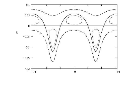
Figure 8: Phase-plane portrait $U=U(\theta,H_{g})$ at $\gamma_{0}=1$, $\epsilon=0.2$, $\kappa=1$ and $\omega=-0.04$. Solid line is for $H=0$, dashed line for $H=-0.04$, dotted line for $H=0.00085$.

Then for $\theta$ we have the following equation

$$\theta_{x}=\omega-\frac{\epsilon}{2}\cos{\theta},$$ (24)

with $U$ determined as

$$U=-\frac{2\omega-\epsilon\cos{\theta}}{3\gamma_{0}+2\kappa\cos{\theta}}.$$ (25)

Integrating Eq.(24) provided that $|\tan(\theta/2)|<\gamma$ we find

$$\cos{\theta}=\frac{1-\gamma^{2}\tanh^{2}(\beta x)}{1+\gamma^{2}\tanh^{2}(\beta x)},$$ (26)

where

$$\gamma=\sqrt{\frac{\epsilon-2\omega}{\epsilon+2\omega}},\quad\beta=\frac{\sqrt{\epsilon^{2}-4\omega^{2}}}{4}.$$

From Eq.(25) we obtain expression for the amplitude U

$$U(x)=\frac{\epsilon-2\omega}{(3\gamma_{0}+2\kappa)\cosh^{2}(\beta x)+(3\gamma_{0}-2\kappa)\gamma^{2}\sinh^{2}(\beta x)}.$$ (27)

Finally the gap solution takes the form

$$u(x,t)=2\sqrt{U}\cos\left(x-\frac{\theta(x)}{2}\right)e^{-i(\omega+1)t},$$ (28)

with

$$-\epsilon/2<\omega<\epsilon/2.$$ (29)

The number of atoms in the soliton is

$$N=\int_{-\infty}^{\infty}|u(x,t)|^{2}dx=2\int_{-\infty}^{\infty}Udx.$$ (30)

When $3\gamma_{0}>2\kappa$

$$N=\frac{8}{\sqrt{9\gamma_{0}^{2}-4\kappa^{2}}}\arctan\frac{(3\gamma_{0}-2\kappa)\gamma}{\sqrt{9\gamma_{0}^{2}-4\kappa^{2}}},$$ (31)

and when $3\gamma_{0}<2\kappa$

$$N=\frac{8}{\sqrt{4\kappa^{2}-9\gamma_{0}^{2}}}\ln\left|\frac{3\gamma_{0}+2\kappa+\gamma\sqrt{4\kappa^{2}-9\gamma_{0}^{2}}}{3\gamma_{0}+2\kappa-\gamma\sqrt{4\kappa^{2}-9\gamma_{0}^{2}}}\right|$$ (32)

In the case

$$3\gamma_{0}>2\kappa$$ (33)

solution (27) is stable for all values of $\omega$ within condition (29), i.e. the soliton exists everywhere in the gap.

In the case $3\gamma_{0}<2\kappa$ for stable solutions we have another condition for $\omega$

$$-\frac{3\epsilon\gamma_{0}}{4\kappa}<\omega<\frac{\epsilon}{2}.$$ (34)

Chemical potential $\omega$ versus norm $N$ is depicted in Fig.9.

Figure 9: The chemical potential $\omega$ versus norm $N$. The curve (a) corresponds to condition (33) and the curve (b) to (34).

According to the Vakhitov-Kolokolov criterionVK the soliton is stable provided that $dN/d\omega<0$.

Evolution of the stable solution for $\gamma_{0}=1$, $\epsilon=0.2$ is given in Fig. 10, The initial wave packet envelope is taken in the form of Eq.(27).

Figure 10: Stable solution for $\gamma_{0}=1$, $\epsilon=0.2$, $\kappa=1$ and $\omega=0.05$ at different times : (a) $t=0$ and (b) $t=100$. The initial wave packet envelope is taken in the form of Eq.(27).

An interesting case we have when $\gamma_{0}=0$. It can be realized with the Feshbach resonance method. Then the soliton exists in the interval $0<\omega<\epsilon/2$, i.e. in the upper half of the gap. The number of atoms for $\omega=\Delta\ll\epsilon$ near the center of the gap can be estimated as

$$N\approx\frac{4}{\pi}\ln|\frac{\epsilon}{\Delta}|.$$

When $\omega=\epsilon/2-\Delta$, i.e. the parameter near the band edge, the number of atoms in gap soliton tends to zero like

$$N\rightarrow\frac{4}{\pi}\sqrt{\frac{\Delta}{\epsilon}}.$$

Numerical simulation of this case is shown in Fig. 11.

Figure 11: Stable solution for $\gamma_{0}=0$, $\epsilon=0.2$, $\kappa=1$ and $\omega=0.05$ at different times : (a) $t=0$ and (b) $t=100$. The initial wave packet envelope is taken in the form Eq.(27).

We performed numerical simulations of the GP equation with the linear-nonlinear optical potentials. In Figs. 10, 11 evolution of the initial state in Eq.(3) is given in the form of Eq.(27).

When $|\tan(\theta/2)|>\gamma$ the expressions for the amplitude $U$ and $\cos\theta$ take the forms

$$\cos{\theta}=\frac{\tanh^{2}(\beta x)-\gamma^{2}}{\tanh^{2}(\beta x)+\gamma^{2}},$$ (35)

$$U(x)=-\frac{\epsilon-\omega}{(3\gamma_{0}+2\kappa)\sinh^{2}(\beta x)+(3\gamma_{0}-2\kappa)\gamma^{2}\cosh^{2}(\beta x)}.$$ (36)

In this case the solution is evidently unstable. Indeed, in this case $dN/d\omega>0$ and in accordance with the Vakhitov-Kolokolov criterionVK such a solution is unstable. PDE simulation of the evolution of an unstable solution for $\gamma_{0}=1$, $\epsilon=0.2$ and $\kappa=2$ is given in Fig. 12, The initial wave packet envelope is taken in the form of Eq.(36).

Figure 12: Unstable solution for $\gamma_{0}=1$, $\epsilon=0.2$, $\kappa=2$ and $\omega=-0.08$ at different times : (a) $t=0$, (b) $t=40$ and (c) $t=140$. The initial wave packet envelope is taken in the form Eq.(36).

V Travelling gap-soliton solution. Solitons collision

Travelling solitons can be obtained proceeding from the anzatz of workIizuka . The solution of Eqs.(II-II) should be sought in the form of the sum of travelling waves with different amplitudes and phases

$$A(x,t)=\sqrt{\Delta}\sqrt{F_{A}(\xi)}e^{i(\theta_{A}(\xi)-\omega t)},$$ (37)

$$B(x,t)=\frac{1}{\sqrt{\Delta}}\sqrt{F_{B}(\xi)}e^{i(\theta_{B}(\xi)-\omega t)},$$ (38)

where

$$\Delta=\sqrt{\frac{2+v}{2-v}},\ \xi=x-vt.$$

Substituting these expressions into Eqs.(II-II) we have

$$F_{\xi}=\frac{\widetilde{\epsilon}}{2}F\sin({\theta_{B}-\theta_{A}})-\widetilde{\kappa}F^{2}\sin({\theta_{B}-\theta_{A}}),$$ (39)

$$(\theta_{B}-\theta_{A})_{\xi}=-\widetilde{\omega}+\frac{\widetilde{\epsilon}}{2}\cos({\theta_{B}-\theta_{A}})-$$

$$3\widetilde{\gamma_{0}}F-2\widetilde{\kappa}F\cos({\theta_{B}-\theta_{A}}),$$ (40)

$$(\theta_{B}+\theta_{A})_{\xi}=\frac{v}{2}\Bigl{[}\widetilde{\omega}+\frac{8}{4+v^{2}}\widetilde{\gamma}_{0}F+$$

$$\widetilde{\kappa}F\cos(\theta_{B}-\theta_{A})\Bigr{]},$$ (41)

where $F=F_{A}=F_{B}$ ,

$$\widetilde{\omega}=\lambda^{2}\omega,\quad\widetilde{\epsilon}=\lambda\epsilon,\quad\widetilde{\kappa}=\lambda^{2}\kappa,$$

$$\widetilde{\gamma}_{0}=\frac{(4+v^{2})}{4}\lambda^{3}\gamma_{0},\quad\lambda=\frac{1}{\sqrt{1-\displaystyle\frac{v^{2}}{4}}}.$$ (42)

The first two equations of this system coincide with Eqs. (20-21) with renormalized parameters. Thus the region of the solitons stability are determined again by conditions Eqs.(29), (34) with renormalized parameters as in Eq.(V).

The gap is given by

$$-\frac{\epsilon}{2}\sqrt{1-\frac{v^{2}}{4}}<\omega<\frac{\epsilon}{2}\sqrt{1-\frac{v^{2}}{4}}.$$ (43)

When the velocity tends to the limiting value $v\rightarrow 2$, the gap region shrinks to zero. Also the gap does not exist for the velocity $v>2$.

The stability condition is

$$-\frac{3(4+v^{2})\epsilon\gamma_{0}}{4\kappa}<\omega<\frac{\epsilon}{2}\sqrt{1-\frac{v^{2}}{4}}.$$ (44)

Numerical simulations with the initial wave packet taken in the form

$$u(x,t)=(A(\xi)e^{ix}+B(\xi)e^{ix})e^{-i(\omega+1)t}$$ (45)

show that obtained solution of Eq.(3) has the form of an automodel soliton.

In the course of evolution of the initial wave-packet the soliton parameters, the soliton speed, amplitude and width, approach their stationary values. Evolution of the soliton speed is shown in Fig. 13.

Figure 13: The time dependence of the travelling soliton speed for $\gamma_{0}=1$, $\epsilon=0.2$, $\kappa=1$ and $\omega=0.05$ when the initial speed $v=0.2$.

To check the nature of obtained moving solutions in Fig. 14 the result of simulation of two solitary waves collision taken in the form of Eq.(45) is shown.

Figure 14: Collision of two moving solitons for $\gamma_{0}=1$, $\epsilon=0.2$, $\kappa=1$ and $\omega=0.05$.

As is evident from this figure, collision of two solitons is nearly elastic. A small radiation at the solitons tails seems to be caused by the nonintegrability of the system.

VI Conclusion

In conclusion, we have investigated the dynamics of BEC under joint action of the linear and nonlinear optical lattices. These lattices can be created by counter propagating laser beams via optically induced Feshbach resonances. Also such structures can be generated in arrays of the Fermi-Bose mixtures. For the case of shallow lattices we derive the coupled mode system of equations and have investigated the modulational instability of cw matter waves in such periodic media. We find the instability regions of cw nonlinear matter waves. The knowledge of MI regions can be useful for generation of gap solitons in such structures. New types of gap soliton solutions are found and the stability regions are analyzed. In particular, the gap soliton can exist in the upper half of the forbidden gap, when the background atomic scattering length is equal to zero($\gamma_{0}=0$). We find the travelling gap soliton solution in BEC and study collision of gap solitons by numerical simulations. It is shown that the collisions are nearly elastic, with the emitting of small radiation, due to the nonintegrability of the couple-mode system.

References

• (1) O. Morsh and M. Oberthaler, Rev.Mod.Phys. 78, 179 (2006).
• (2) V.A. Brazhnyi and V.V. Konotop, Mod.Phys.Lett. B 18, 627 (2004).
• (3) F.Kh. Abdullaev and M. Salerno, J.Phys. B 36, 2851 (2003).
• (4) G. Theocharis, P. Schmelcher, P.G. Kevrekidis, and D.J. Frantzeskakis, Phys.Rev. A 72, 033614 (2005).
• (5) F.Kh. Abdullaev, A. Gammal, A.M. Kamchatnov, and L. Tomio, Int.J. Mod.Phys. B 19, 3415 (2005).
• (6) J. Garnier and F.Kh. Abdullaev, Phys.Rev. A 74, 013604 (2006).
• (7) H. Sakaguchi and B.A. Malomed, Phys.Rev. E 72, 046610 (2005).
• (8) F.Kh. Abdullaev and J. Garnier, Phys.Rev. A 72 061605(R) (2005).
• (9) G. Fibich, Y. Sivan, and M.I. Weinstein, Physica D 217, 31 (2006).
• (10) M. Theis, G. Thalhammaer, K. Winkler, M. Hellwig, G. Ruff, R. Grimm, and J.H. Denshlag, Phys.Rev.Lett. 93, 123001 (2004).
• (11) P.O. Fedichev, Yu. Kagan, G.V. Shlyapnikov, and J.T.M. Walraven, Phys.Rev.Lett. 77, 2913 (1996).
• (12) Yu. Bludov and V.V. Konotop, arXive cond-mat/0606815.
• (13) B.A. Malomed, T. Mayteevarunyoo, E. Ostrovskaya, and Y.S. Kivshar, Phys.Rev.E 71, 056616 (2005).
• (14) A.B. Aceves and S. Wabnitz, Phys.Lett. A 141, 37 (1989); D.N. Christodoulides and R.I. Joseph, Phys.Rev.Lett. 62, 1746 (1989).
• (15) T. Iizuka and C.M. de Sterke, Phys.Rev. E 61, 4491 (2000).
• (16) D. Pelinovsky, J. Sears, L. Brzozowski, and E.H. Sargent, J.Opt.Soc.Am. B 19, 43 (2002).
• (17) C.M. de Sterke and J.E. Sipe, Progress in Optics, 33, 203 (1994).
• (18) A.V. Yulin and D.V. Skryabin, Phys.Rev. A 67, 023611 (2003).
• (19) N.K. Efremidis and C.N. Christodoulides, Phys.Rev. A 67, 063608 (2003).
• (20) B.J. Eggleton, R.R. Slusher, C.M. de Sterke, P.A. Krug, and J.E. Sipe, Phys.Rev.Lett. 76, 1627 (1996).
• (21) A. Trombettoni and A. Smerzi, Phys.Rev.Lett. 86, 2353 (2001).
• (22) F.Kh. Abdullaev, B.B.Baizakov, S.A. Darmanyan, V.V. Konotop, and M. Salerno, Phys.Rev. A 64, 043606 (2001).
• (23) A. Khare, K.O. Rasmussen, M. Salerno, M.R. Samuelsen, and A. Saxena, Phys.Rev.E 74, 016607 (2006).
• (24) F.Kh. Abdullaev, S.A. Darmanyan, and J. Garnier, In Progress in Optics, 44, 303 (2002).
• (25) V.V. Konotop and M. Salerno, Phys.Rev.A 65, 021602 (2002).
• (26) C.M. de Sterke, J.Opt.Soc.Am. B 15, 2660 (1998).
• (27) K. Porsezian and K. Senthilnathan, Chaos 15, 037109 (2005).
• (28) M. Chugunova and D. Pelinovsky, SIAM J. Appl. Dyn. Sys. 5, 66 (2006).
• (29) N.G. Vakhitov and A.A. Kolokolov, Radiophysics and Quantum Electronics, 16, 783 (1973).
• (30) F.Kh. Abdullaev and M. Salerno, Phys.Rev. A 72, 033617 (2005).