Quantum vacuum radiation spectra from a semiconductor microcavity
with a time-modulated vacuum Rabi frequency

Abstract

We develop a general theory of the quantum vacuum radiation generated by an arbitrary time-modulation of the vacuum Rabi frequency for an intersubband transition of a doped quantum well system embedded in a semiconductor planar microcavity. Both non-radiative and radiative losses are included within an input-output quantum Langevin framework. The intensity and the main spectral signatures of the extra-cavity emission are characterized as a function of the amplitude and the frequency of the vacuum modulation. A significant amount of photon pairs, which can largely exceed the black-body radiation in the mid and far infrared, is shown to be produced with realistic parameters. For a large amplitude resonant modulation, a parametric oscillation regime can be also achieved.

The radiation generated by a time-modulation of the quantum vacuum is a very general and fascinating phenomenon, and has been predicted to occur in a variety of physical systems ranging from non-uniformly accelerated boundaries (dynamical Casimir effect  RMP ; dyn_Casimir ) to semiconductors with rapidly changing dielectric properties Yablonovitch . These quantum vacuum phenomena have some analogies with the Unruh-Hawking radiationHawking in the curved space-time around a black hole. Recent years have seen the appearance of a number of proposals to enhance the intensity of the quantum vacuum radiation, exploting, e.g., high-finesse Fabry-Pérot  resonatorsReynaud , a time-modulation of the dielectric constant of a monolithic solid-state cavity epsilon_var , or even the reflectivity change of semiconductor mirrors induced by an ultrafast photogeneration of carriers Braggio . Still, the very weak intensity of the emitted radiation has so far hindered its experimental observation.

Planar semiconductor microcavities embedding a doped multiple quantum well structure have attracted a considerable interest in the last few years. As demonstrated by several spectroscopic experiments in the mid infrared range Dini_PRL ; Dupont ; Aji_APL ; SNS_unpub ; SST ; Luca , the strong coupling between the cavity mode and the electronic transition between the first two quantum well subbands results in an elementary excitation spectrum consisting of intersubband polaritons, i.e. linear superpositions of cavity photon and intersubband excitation states. The most interesting property of these systems from the point of view of the quantum vacuum radiation is given by the large vacuum Rabi frequency $\Omega_{R}$, being as high as a significant fraction of the intersubband transition frequency $\omega_{12}$ Ciuti_vacuum . In this unusual ultrastrong coupling regime Ciuti_vacuum ; Ciuti_PRA , the antiresonant terms of the vacuum Rabi coupling play in fact a significant role and the quantum ground state of the system is a squeezed vacuum state containing a significant amount of correlated pairs of cavity photons. The photon pairs in the ground state are virtual and cannot escape the cavity if its parameters are time-independentCiuti_PRA .

In order to release these bound photons into extracavity radiation, the quantum vacuum has to be modulated in time. The recent experimental demonstration of a wide tunability of the cavity parameters (in particular of the vacuum Rabi frequency $\Omega_{R}$ Aji_APL ) via an external gate bias and the possibility of ultrafast modulation SNS_unpub makes the present system a very promising one in view of the observation of quantum vacuum radiation. A first theoretical study for an ideal isolated cavity Ciuti_vacuum has indeed suggested that a non-adiabatic switch-off of $\Omega_{R}$ results in a significant number of photon pairs being emitted from the cavity.

A general theory which includes the effect of non-radiative and radiative losses for arbitrary time-modulations is however still missing, as well as a complete characterization of the intensity and spectral signatures of the emitted radiation for realistic cavity systems. In this letter, we address these fundamental issues by developing a theory of the quantum vacuum radiation for an arbitrary modulation of the microcavity properties. The properties of the extracavity emission for the most promising case of a periodic modulation of $\Omega_{R}$ are calculated by means of the generalized input-output formalism Ciuti_PRA : remarkably, the emitted quantum vacuum radiation turns out to be much stronger than the radiation by spurious effects such as black body emission. The instability regions in which the vacuum modulation produces a parametric oscillation of the cavity field are identified and shown to be within experimental reach.

A theoretical description of the system can be obtained by means of the formalism developed in Ciuti_vacuum ; Ciuti_PRA . The photon mode in the planar microcavity and the bright intersubband electronic excitation of the doped quantum well system (see Fig. 1) are described as two bosonic modes. Given the translational symmetry of the system along the cavity plane, the in-plane wavevector ${\mathbf{k}}$ is a good quantum number. The creation operators for respectively a cavity photon and an electronic excitation of wavevector ${\mathbf{k}}$ are denoted by $\hat{a}^{\dagger}_{\mathbf{k}}$ and $\hat{b}^{\dagger}_{\mathbf{k}}$. The in-plane dispersion relation of the cavity-photon is defined as $\omega_{c,{\mathbf{k}}}$, while the frequency $\omega_{12}$ of the intersubband excitation is taken dispersionless. As explained in detail in Ref. Ciuti_vacuum , the electric-dipole coupling between one cavity photon and one bright intersubband excitation is quantified by the vacuum Rabi frequency $\Omega_{R,k}=\left(\frac{2\pi e^{2}}{\epsilon_{\infty}m_{0}L^{\rm eff}_{\rm cav}}~{}\sigma_{el}~{}N^{eff}_{QW}~{}f_{12}\sin^{2}\theta\right)^{1/2}~{}$, where $L^{\rm eff}_{\rm cav}$ is the effective length of the cavity mode, $\epsilon_{\infty}$ the dielectric constant of the cavity spacer, $\sigma_{el}$ the density of the two-dimensional electron gas, $N^{eff}_{QW}$ the effective number of quantum wells, $f_{12}$ the oscillator strength of the intersubband transition and $\theta$ is the intracavity photon propagation angle such that $\sin\theta=ck/(\omega_{12}\sqrt{\epsilon_{\infty}})$.

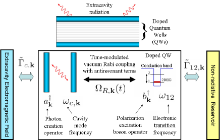
Figure 1: (color online). Top: a sketch of the considered semiconductor planar microcavity system. Bottom: a scheme of the quantum model.

The second quantization Hamiltonian of the present cavity system reads

$$H=\frac{1}{2}\,\hat{v}^{\dagger}_{{\mathbf{k}}}\,\eta\,{\mathcal{M}}_{\mathbf{k}}\,\hat{v}_{{\mathbf{k}}}$$ (1)

where the column vector of operators $\hat{v}_{{\mathbf{k}}}$ is defined as $\hat{v}_{{\mathbf{k}}}\equiv(\hat{a}_{{\mathbf{k}}},\hat{b}_{{\mathbf{k}}},\hat{a}^{\dagger}_{-{\mathbf{k}}},\hat{b}^{\dagger}_{-{\mathbf{k}}})^{T}$, $\eta$ is the diagonal metric $\eta=\textrm{diag}[1,1,-1,-1]$ and the Hopfield-Bogoliubov matrix ${\mathcal{M}}_{\mathbf{k}}$ is defined as

$${\mathcal{M}}_{\mathbf{k}}\equiv\left(\begin{array}[]{cccc}\omega_{c,{\mathbf{k}}}+2D_{{\mathbf{k}}}&i\Omega_{R,{\mathbf{k}}}&2D_{{\mathbf{k}}}&-i\Omega_{R,{\mathbf{k}}}\\ -i\Omega_{R,{\mathbf{k}}}&\omega_{12}&-i\Omega_{R,{\mathbf{k}}}&0\\ -2D_{{\mathbf{k}}}&-i\Omega_{R,{\mathbf{k}}}&-\omega_{c,{\mathbf{k}}}-2D_{{\mathbf{k}}}&i\Omega_{R,{\mathbf{k}}}\\ -i\Omega_{R,{\mathbf{k}}}&0&-i\Omega_{R,{\mathbf{k}}}&-\omega_{12,{\mathbf{k}}}\\ \end{array}\right).$$

For a quantum well, the diamagnetic coupling constant is approximately $D_{{\mathbf{k}}}\simeq\Omega_{R,{\mathbf{k}}}^{2}/\omega_{12}$ Ciuti_vacuum . The ultra-strong coupling regime is characterized by a value of $\Omega_{R,{\mathbf{k}}}$ comparable to $\omega_{c,{\mathbf{k}}}$ and $\omega_{12}$. In this regime, a central role is played by the anti-resonant light-matter coupling terms corresponding to the off-diagonal (1,3), (1,4), (2,3), (2,4) terms of ${\mathcal{M}}$ (and their transposed). In the following, a general time-dependence of the Rabi frequency is considered: $\Omega_{R,{\mathbf{k}}}(t)=\bar{\Omega}_{R,{\mathbf{k}}}+\Omega^{mod}_{R,{\mathbf{k}}}(t)$ and $D_{k}(t)=\bar{D}_{k}+D^{mod}_{k}(t)$.

Non-radiative as well as radiative losses will be taken into account by means of the generalized input-output formalism developed in Ciuti_PRA : the system is in interaction with two baths of harmonic oscillators, which are responsible for dissipation and fluctuations of both the cavity-photon and the electronic polarization fields. The radiative and non-radiative complex damping rates are denoted by ${\tilde{\Gamma}}_{c,{\mathbf{k}}}(\omega)$ and ${\tilde{\Gamma}}_{12,{\mathbf{k}}}(\omega)$. The real part (zero for $\omega<0$ Ciuti_PRA ) quantifies the frequency-dependent losses, while the imaginary part represents the Lamb-shift of the mode due to the coupling to the external bath. The resulting quantum Langevin equations are conveniently written in frequency space as the vector equation:

$$\int_{-\infty}^{+\infty}\!\!\!\!d\omega^{\prime}\,\left[\bar{\mathcal{M}}_{{\mathbf{k}},\omega}\,\delta(\omega-\omega^{\prime})+{\mathcal{M}}^{mod}_{{\mathbf{k}},\omega-\omega^{\prime}}\right]\,\tilde{v}_{{\mathbf{k}}}(\omega^{\prime})=-i\tilde{\mathcal{F}}_{{\mathbf{k}}}$$ (2)

where $\tilde{v}_{\mathbf{k}}(\omega)$ is the Fourier transform of the operator vector $\hat{v}_{\mathbf{k}}(t)$ and the quantum Langevin operator vector

$$\tilde{\mathcal{F}}_{{\mathbf{k}}}=\left(\tilde{F}_{c,{\mathbf{k}}}(\omega),\tilde{F}_{12,{\mathbf{k}}}(\omega),\tilde{F}^{\dagger}_{c,-{\mathbf{k}}}(-\omega),\tilde{F}^{\dagger}_{12,-{\mathbf{k}}}(-\omega)\right)^{T}$$

takes into account the quantum fluctuations due to the coupling to the baths. The matrix

$$\bar{\mathcal{M}}_{{\mathbf{k}},\omega}={\mathcal{M}}_{\mathbf{k}}-\mathbf{1}\,\omega\\ -i\,\textrm{diag}[\tilde{\Gamma}_{c,{\mathbf{k}}}(\omega),\tilde{\Gamma}_{12,{\mathbf{k}}}(\omega),\tilde{\Gamma}^{*}_{c,-{\mathbf{k}}}(-\omega),\tilde{\Gamma}^{*}_{12,-{\mathbf{k}}}(-\omega)]$$ (3)

summarizes the time-independent properties of the system, while ${{\mathcal{M}}}^{mod}_{{\mathbf{k}},\omega}$ describes the time-modulation. For the case of a time-dependent vacuum Rabi frequency $\Omega_{R,{\mathbf{k}}}(t)$, this has the form:

$${{\mathcal{M}}}^{mod}_{{\mathbf{k}},\omega}=\left(\begin{array}[]{cccc}2\tilde{D}^{mod}_{{\mathbf{k}},\omega}&i\tilde{\Omega}^{mod}_{R,{\mathbf{k}},\omega}&2\tilde{D}^{mod}_{{\mathbf{k}},\omega}&-i\tilde{\Omega}^{mod}_{R,{\mathbf{k}},\omega}\\ -i\tilde{\Omega}^{mod}_{R,{\mathbf{k}},\omega}&0&-i\tilde{\Omega}^{mod}_{R,{\mathbf{k}},\omega}&0\\ -2\tilde{D}^{mod}_{{\mathbf{k}},\omega}&-i\tilde{\Omega}^{mod}_{R,{\mathbf{k}},\omega}&-2\tilde{D}^{mod}_{{\mathbf{k}},\omega}&i\tilde{\Omega}^{mod}_{R,{\mathbf{k}},\omega}\\ -i\tilde{\Omega}^{mod}_{R,{\mathbf{k}},\omega}&0&-i\tilde{\Omega}^{mod}_{R,{\mathbf{k}},\omega}&0\end{array}\right)~{},$$

where ${\tilde{\Omega}}^{mod}_{R,{\mathbf{k}},\omega}$ and $\tilde{D}_{{\mathbf{k}},\omega}^{mod}$ are the Fourier transforms of respectively $\Omega^{mod}_{R,{\mathbf{k}}}(t)$ and $D_{\mathbf{k}}^{mod}(t)$.

The exact solution of (2) is given by

$$\tilde{v}_{{\mathbf{k}}}(\omega)=-i\int_{-\infty}^{\infty}d\omega^{\prime}{{\mathcal{G}}}_{{\mathbf{k}}}(\omega,\omega^{\prime})\tilde{\mathcal{F}}_{{\mathbf{k}}}(\omega^{\prime})~{},$$ (4)

where ${\mathcal{G}}_{{\mathbf{k}}}(\omega,\omega^{\prime})$ is the inverse of ${{\mathcal{M}}}_{{\mathbf{k}}}(\omega,\omega^{\prime})\equiv\bar{\mathcal{M}}_{{\mathbf{k}},\omega^{\prime}}\delta(\omega-\omega^{\prime})+{{\mathcal{M}}}^{mod}_{{\mathbf{k}},\omega-\omega^{\prime}}$, i.e.,

$$\int_{-\infty}^{\infty}d\omega^{\prime}\sum_{s}{\mathcal{G}}^{rs}_{{\mathbf{k}}}(\omega,\omega^{\prime}){{\mathcal{M}}}_{{\mathbf{k}}}^{st}(\omega^{\prime},\omega^{\prime\prime})\equiv\delta_{rt}\delta(\omega-\omega^{\prime\prime}).$$

Using the input-output scheme Ciuti_PRA , we obtain the spectral density of emitted photons from the cavity $S_{\mathbf{k}}^{out}(\omega)$ as a function of the incident one $S_{\mathbf{k}}^{in}(\omega)$ and the quantum Langevin forces $\tilde{\mathcal{F}}_{{\mathbf{k}}}$:

$$S_{{\mathbf{k}}}^{out}(\omega)=S_{{\mathbf{k}}}^{in}(\omega)-\frac{i}{2\pi}\int_{-\infty}^{\infty}d\omega^{\prime}\sum_{s}{{\mathcal{G}}}_{{\mathbf{k}}}^{*1s}(\omega,\omega^{\prime})\tilde{\mathcal{F}}_{{\mathbf{k}}}^{\dagger\,s}(\omega^{\prime})\tilde{\mathcal{F}}_{{\mathbf{k}}}^{1}(\omega)+\frac{i}{2\pi}\int_{-\infty}^{\infty}d\omega^{\prime}\sum_{s}{{\mathcal{G}}}^{1s}_{{\mathbf{k}}}(\omega,\omega^{\prime})\tilde{\mathcal{F}}^{\dagger\,1}_{{\mathbf{k}}}(\omega)\tilde{\mathcal{F}}_{{\mathbf{k}}}^{s}(\omega)\\ +\frac{1}{\pi}\Re(\tilde{\Gamma}_{c,{\mathbf{k}}}(\omega))\int_{-\infty}^{\infty}\!\!\!d\omega^{\prime}\,\int_{-\infty}^{\infty}\!\!\!d\omega^{\prime\prime}\,\sum_{rs}\bar{{\mathcal{G}}}_{{\mathbf{k}}}^{*1r}(\omega,\omega^{\prime}){{\mathcal{G}}}_{{\mathbf{k}}}^{1s}(\omega,\omega^{\prime\prime})\tilde{\mathcal{F}}_{{\mathbf{k}}}^{\dagger\,r}(\omega^{\prime})\tilde{\mathcal{F}}_{{\mathbf{k}}}^{s}(\omega^{\prime\prime})~{}.$$ (5)

If one is interested in the quantum vacuum radiation due to the time-modulation of the cavity parameters, a vacuum state has to be considered for the input state, so that $\langle S_{\mathbf{k}}^{in}(\omega)\rangle=0$, and the fluctuating quantum Langevin forces acting on the cavity-photon and the electronic polarization modes ($j,j^{\prime}\in\{c,12\}$) are such that:

$$\left\langle\tilde{F}_{j,{\mathbf{k}}}(\omega)\,\tilde{F}^{\dagger}_{j^{\prime},{\mathbf{k}}^{\prime}}(\omega^{\prime})\right\rangle = 4\pi\,\delta(\omega-\omega^{\prime})\,\delta_{jj^{\prime}}\,\textrm{Re}[\Gamma_{j,{\mathbf{k}}}(\omega)]\,\delta_{{\mathbf{k}},{\mathbf{k}}^{\prime}}$$

$$\left\langle\tilde{F}^{\dagger}_{j,{\mathbf{k}}}(\omega)\,\tilde{F}_{j^{\prime},{\mathbf{k}}^{\prime}}(\omega^{\prime})\right\rangle = \left\langle\tilde{F}_{j,{\mathbf{k}}}(\omega)\,\tilde{F}_{j^{\prime},{\mathbf{k}}^{\prime}}(\omega^{\prime})\right\rangle=0.$$ (6)

This implies that only the last term of (5) gives a finite contribution to the emitted radiation. After some algebra, we get :

$$\langle S_{{\mathbf{k}}}^{out}(\omega)\rangle=4\Re(\tilde{\Gamma}_{c,{\mathbf{k}}}(\omega))\int_{0}^{\infty}\!\!\!\!\!d\omega^{\prime}\,\left\{\lvert\bar{{\mathcal{G}}}_{{\mathbf{k}}}^{13}(\omega,-\omega^{\prime})\rvert^{2}\Re[\tilde{\Gamma}_{c,{\mathbf{k}}}(\omega^{\prime})]\right.\\ \left.+\lvert\bar{{\mathcal{G}}}_{{\mathbf{k}}}^{14}(\omega,-\omega^{\prime})\rvert^{2}\Re[\tilde{\Gamma}_{12,{\mathbf{k}}}(\omega^{\prime})]\right\}~{}.$$ (7)

The total number of emitted photons with in-plane wave-vector ${\mathbf{k}}$ is given by $N^{out}_{{\mathbf{k}}}=\int_{-\infty}^{\infty}\langle S_{{\mathbf{k}}}^{out}(\omega)\rangle d\omega$. Note that in the absence of anti-resonant couplings in the Hamiltonian (1), $\bar{{\mathcal{G}}}_{{\mathbf{k}}}^{13}=\bar{{\mathcal{G}}}_{{\mathbf{k}}}^{14}=0$ giving a vanishing emitted radiation.

This general theory can be applied to calculate the intensity of quantum vacuum radiation emitted by the cavity for an arbitrary modulation of the cavity parameters and for arbitrary frequency-dependent losses. In the following, we shall focus ourselves on the case of a periodic modulation of the vacuum Rabi frequency, i.e.

$$\Omega^{mod}_{R,{\mathbf{k}}}(t)=\Delta\Omega_{R,{\mathbf{k}}}\cos(\omega_{mod}t).$$ (8)

If the modulation frequency is tuned on resonance with the cavity modes, one expects Reynaud that the quantum vacuum radiation can be strongly enhanced as compared to the case of a single sudden change of $\Omega_{R,{\mathbf{k}}}$ discussed in Ciuti_vacuum . In the stationary state, the relevant quantity to characterize the intensity of the emission is the total number of photons emitted per unit time $dN^{out}_{\mathbf{k}}/dt$.

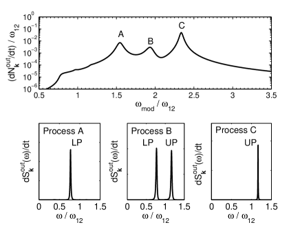
Figure 2: Top panel: rate of emitted photons $dN_{{\mathbf{k}}}^{out}/dt$ (in units of $\omega_{12}$) as a function of the normalized modulation frequency $\omega_{mod}/\omega_{12}$. Parameters: $(\omega_{c,{\mathbf{k}}}+2D_{k})/\omega_{12}=1$, $\Gamma/\omega_{12}=0.025$, $\bar{\Omega}_{R,{\mathbf{k}}}/\omega_{12}=0.2$, $\Delta\Omega_{R,{\mathbf{k}}}/\omega_{12}=0.04$. Note that, due to the scaling properties of the present model, the results do not depend on the specific value of $\omega_{12}$. The letters A,B,C indicate three different resonantly enhanced processes. Bottom panels: the spectral density (arb. u.) for the processes A, B, C respectively. The resonant peaks occur at the LP (Lower Polariton) and/or UP (Upper Polariton) frequency.

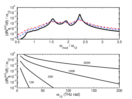
Figure 3: (color online). Top panel: rate $dN^{out}_{\mathbf{k}}/dt$ (in units of $\omega_{12}$) of emitted photons as a function of $\omega_{mod}/\omega_{12}$ for different values of the damping $\Gamma/\omega_{12}=0.025$ (solid), $0.05$ (dashed), $0.075$ (dot-dashed). Other parameters as in Fig. 2. Bottom panel: normalized rate of emitted photons from a black-body emitter as a function of $\omega_{12}$ for different temperatures.

Predictions for the rate $dN^{out}_{\mathbf{k}}/dt$ (in units of $\omega_{12}$) of emitted photons as a function of the modulation frequency $\omega_{mod}$ are shown in the top panel of Fig.2. For the sake of simplicity, a frequency-independent damping rate has been considered $\Re\{\tilde{\Gamma}_{c,{\mathbf{k}}}(\omega>0)\}=\Re\{\tilde{\Gamma}_{12,{\mathbf{k}}}(\omega>0)\}=\Gamma$; the imaginary part has been consistently determined via the Kramers-Kronig relations Ciuti_PRA . Values inspired from recent experiments Dini_PRL ; Aji_APL ; SNS_unpub have been used for the cavity parameters. The structures in the integrated spectrum shown in the top panel of Fig.2 can be identified as resonance peaks when the modulation is phase-matched. Indeed, the vacuum modulation induces the creation of pairs of real cavity polaritons. This sort of nonlinear parametric process is enhanced when the phase-matching condition $r\,\omega_{mod}=\omega_{j,{\mathbf{k}}}+\omega_{j^{\prime},-{\mathbf{k}}}$ is fulfilled, $r$ being a generic positive integer number, and $j,j^{\prime}\in\{LP,UP\}$. The dominant features A,B,C are the three lowest-order $r=1$ peaks corresponding to the processes where either two Lower Polaritons (LPs), or one LP and one Upper Polariton (UP), or two UP’s are generated. This interpretation is supported by the spectral densities plotted in the three lower panels of Fig.2 for modulation frequencies corresponding to respectively A,B,C peaks. In each case, the emission is strongly peaked at the frequencies of the final polariton states involved in the process; for the parameter chosen, we have indeed Ciuti_vacuum ; Ciuti_PRA $\omega_{LP,{\mathbf{k}}}\simeq\omega_{12}-\bar{\Omega}_{R,{\mathbf{k}}}=0.8\,\omega_{12}$ for the lower polariton and $\omega_{UP,k}\simeq\omega_{12}+\bar{\Omega}_{R,{\mathbf{k}}}=1.2\,\omega_{12}$ for the upper polariton. The shoulder and the smaller peak at $\omega_{mod}/\omega_{12}<1$ can be attributed to $r=2$ processes, while higher order processes require a weaker damping to be visible.

More insight into the properties of the quantum vacuum emission are given in Fig.3. In the top panel, the robustness of the emission has been verified for increasing values of the damping rate $\Gamma$, the resonant enhancement is quenched, but the main features remain unaffected even for rather large damping rates. In the bottom panel, comparison with the black body emission in the absence of any modulation is made: the total rate of emitted black body photons at given ${\mathbf{k}}$ is shown as a function of $\omega_{12}$ (ranging from the terahertz to the mid infrared range) for ${\mathbf{k}}$ correspoding to an intracavity photon propagation angle of $60^{\circ}$ and different temperatures. Note how the black body emission decreases almost exponentially with $\omega_{12}$, while the quantum vacuum radiation, being a function of $\bar{\Omega}_{R,{\mathbf{k}}}/\omega_{12}$ only, linearly increases with $\omega_{12}$ at fixed $\bar{\Omega}_{R,{\mathbf{k}}}/\omega_{12}$. From this plot, one is quantitatively reassured that for reasonably low temperatures the quantum vacuum radiation can exceed the black-body emission even by several orders of magnitude.

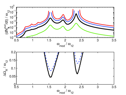
Figure 4: (color online). Top panel: rate $dN^{out}_{\mathbf{k}}/dt$ (in units of $\omega_{12}$) of emitted photons as a function of $\omega_{mod}/\omega_{12}$ for different values of the normalized modulation amplitude $\Delta\Omega_{R,k}/\omega_{12}=0.01,0.04,0.07,0.1$ (from bottom to top). Other parameters as in Fig. 2. Bottom panel: instability boundaries for $\Gamma/\omega_{12}=0.025$ (solid), $0.05$ (dashed). Above the lines, the system is parametrically unstable.

The increase of the emitted intensity versus the modulation amplitude $\Delta\Omega_{R,{\mathbf{k}}}/\omega_{12}$ is shown in the top panel of Fig.4. In particular, note the strongly superlinear increase of the emission intensity around the A and C resonance peaks. In these regions, if the modulation amplitude is large enough, the system can even develop a parametric instability, the incoherent quantum vacuum radiation being replaced by a coherent parametric oscillation OPO . Above the instability threshold, the results obtained from the solution of Eq. (2) in Fourier space are no longer valid, being the field amplitudes exponentially growing with time. Hence they are not shown here. The instability boundaries for parametric oscillation can be calculated applying the Floquet methodFloquet to the mean-field equations for the intracavity fields $\langle a_{{\mathbf{k}}}\rangle$ and $\langle b_{{\mathbf{k}}}\rangle$. The result is shown in the bottom panel of Fig.4 as a function of $\omega_{mod}/\omega_{12}$ and $\Delta\Omega_{R,k}/\omega_{12}$: agreement with the position of the vertical asymptotes of the spectra in the top panel of of Fig.4 is found.

In conclusion, we have presented a complete theory with exact solutions for the quantum vacuum radiation from a semiconductor microcavity with a time-modulated vacuum Rabi frequency. In order to isolate it from spurious effects such as black-body radiation, the main signatures of the quantum vacuum radiation as a function of the modulation parameters have been characterized. Our results show that semiconductor microcavities in the ultrastrong coupling regime are a very promising system for the observation of quantum vacuum radiation phenomena.

References

(1) M. Kardar and R. Golestanian, Rev. Mod. Phys.
71, 1233 (1999).
(2) G. T. Moore, J. Math. Phys. (N.Y.) 11, 2679
(1970); S. A. Fulling and P. C. W. Davies, Proc. R. Soc. London A
348, 393 (1976)
(3) E. Yablonovitch, Phys. Rev. Lett. , 1742 (1989).
(4) W. G. Unruh, Phys. Rev. D 10, 3194 (1974);
S. W. Hawking, Nature (London) 248, 30 (1974).
(5) A. Lambrecht, M. T. Jaekel, and S. Reynaud,
Phys. Rev. Lett. 77, 615 (1996). For a recent review, see:
A. Lambrecht, J. Opt. B: Quantum Semiclass. Opt. 7, S3 (2005).
(6) V. V. Dodonov, A. B. Klimov, D. E. Nikonov,
Phys. Rev. A 47, 4422 (1993); C. K. Law, Phys. Rev. A 49, 433 (1994).
(7) C. Braggio, et al.,
Rev. Sc. Instr. 75, 4967 (2004);
Europhys. Lett. 70 754 (2005).
(8) D. Dini, R. Kohler, A. Tredicucci, G. Biasiol, and L. Sorba,
Phys. Rev. Lett. 90, 116401 (2003).
(9) E. Dupont, H. C. Liu, A. J. SpringThorpe, W. Lai, and M. Extavour, Phys. Rev.
B 68, 245320 (2003).
(10) A. A. Anappara, A. Tredicucci, G. Biasiol, L. Sorba, Appl.
Phys. Lett. 87, 051105 (2005).
(11) R. Colombelli, C. Ciuti, Y. Chassagneux, C.
Sirtori, Semicond. Sci. Technol. 20, 985 (2005).
(12) A. A. Anappara, A. Tredicucci, F. Beltram, G. Biasol, L. Sorba,
Appl. Phys. Lett. 89, 171109 (2006).
(13) L. Sapienza, A. Vasanelli, C. Sirtori et al., in preparation
(14) C. Ciuti, G. Bastard, I. Carusotto, Phys.
Rev. B 72, 115303 (2005).
(15) C. Ciuti, I. Carusotto, Phys. Rev. A 74,
033811 (2006).
(16) D. F. Walls and G. J. Milburn, Quantum
Optics (Springer, Berlin, 1994).
(17) R. Grimshaw, Nonlinear Ordinary Differential equations (CRC Press,
1993).