Phase diagram of an Ising model for ultrathin magnetic films: comparing mean field and Monte Carlo predictions

Abstract

We study the critical properties of a two–dimensional Ising model with competing ferromagnetic exchange and dipolar interactions, which models an ultra-thin magnetic film with high out–of–plane anisotropy in the monolayer limit. In this work we present a detailed calculation of the $(\delta,T)$ phase diagram, $\delta$ being the ratio between exchange and dipolar interactions intensities. We compare the results of both mean field approximation and Monte Carlo numerical simulations in the region of low values of $\delta$, identifying the presence of a recently detected phase with nematic order in different parts of the phase diagram, besides the well known striped and tetragonal liquid phases. We also found that, in the regions of the phase diagram where Monte Carlo simulations display nematic order, the mean field approximation predicts hybrid solutions composed by stripes of different widths. Another remarkable qualitative difference between both calculations is the absence, in this region of the Monte Carlo phase diagram, of the temperature dependency of the equilibrium stripe width predicted by the mean field approximation.

I Introduction

Many ultrathin magnetic films, like e.g. Co/Cu, Co/Au, Fe/Cu, undergo a reorientation transition at a temperature $T_{R}$; for temperatures below $T_{R}$ the spins align preferentially in a direction perpendicular to the film, while above $T_{R}$ they align in a magnetized state parallel to the plane of the film Allenspach et al. (1990); Vaterlaus et al. (2000); De’Bell et al. (2000). This reorientation transition is due to the competition between the in-plane part of the dipolar interaction and the surface anisotropy Politi (1998). Furthermore, in the range of temperatures where the magnetization points out of the plane, the competition between exchange and dipolar interaction causes the global magnetization to be effectively zero but instead striped magnetic domain patterns emergeVaterlaus et al. (2000); Portmann et al. (2003); De’Bell et al. (2000). In the limit of a monolayer film, the following dimensionless Ising Hamiltonian emerges as a minimal model to describe many of the relevant physical properties of those materialsDe’Bell et al. (2000):

$${\cal H}=-\delta\sum_{<i,j>}S_{i}S_{j}+\sum_{(i,j)}\frac{S_{i}S_{j}}{r^{3}_{ij}}$$ (1)

where $\delta$ stands for the ratio between the exchange $J_{0}>0$ and the dipolar $J_{d}>0$ interactions parameters, i.e., $\delta=J_{0}/J_{d}$. The first sum runs over all pairs of nearest neighbor Ising spins $S_{i}=\pm 1$ in a square lattice and the second one over all distinct pairs of spins of the lattice (every pair is counted once); $r_{ij}$ is the distance, measured in crystal units, between sites $i$ and $j$ and the energy is measured in units of $J_{d}$. In spite of intense theoretical workCzech and Villain (1989); De’Bell et al. (2000); MacIsaac et al. (1995); Booth et al. (1995); Stoycheva and Singer (2000); Gleiser et al. (2002); Cannas et al. (2004a, b); Casartelli et al. (2004); Cannas et al. (2006); Rastelli et al. (2006), there are still many important open questions regarding the critical properties of this model. A detailed understanding of those critical properties is the cornerstone of the theoretical framework needed to explain complex phenomena in ultrathin magnetic films, such as the recently observed inverse transition in Fe on Cu filmsPortmann et al. (2003).

The main difficulties to analyze the critical properties of this model are related to the long range character of the dipolar interactions, which combined with the frustration derived from the competition between interactions, adds to any theoretical approach an extra degree of complexity. Then, even the simplest approach, namely mean field approximation (MF), leads to an infinite number of coupled equations that, except for some particular situations cannot be solved exactly. For instance, in an early work Czech and VillainCzech and Villain (1989) derived an exact expression for the MF critical temperature between the disordered and the modulated (striped) phases; however, for sub–critical temperatures the determination of any property must rely on numerical solutions of the mean field equations or further ansatz has to be introducedPortmann et al. (2006) to obtain approximated solutions of the MF equations. An example is the temperature dependency of the equilibrium stripe width; being experimentally accessiblePortmann et al. (2006), reliable theoretical predictions of this property could be very important to understand the basic mechanisms behind the complex behavior observed in these materials. Though MF is a powerful theoretical tool, it is known that, even when the corresponding equations can be solved exactly, neglecting fluctuations can introduce qualitative changes in the critical behavior. Therefore, it is important to compare MF predictions with those obtained by other methods, in order to establish the limits of validity of the approximation.

A natural way to check the mean field predictions is to contrast them with Monte Carlo (MC) simulations. However, the long range order nature of the dipolar interactions makes it very difficult to simulate large system sizes. The ground state stripe width $h$ is the natural length scale in these problems. Hence, in order to avoid strong finite size effects, the simulations must be carried out for system sizes $L\gg h$; this restricts the simulations to situations in which $h$ is much smaller than the experimentally observed values (typical values of the stripe width in Fe on Cu films, for instance, are of the orderWon et al. (2005); Portmann et al. (2006) of $1\,\mu m$, which corresponds roughly to $h=4000$ lattice constants). Since the ground state value of $h$ increases exponentially withYafet and Gyorgy (1988) $\delta$, the values of $\delta$ available for simulations are about of one order of magnitude smaller then the realistic values.

In this work we carry out a detailed analysis of the equilibrium phase diagram of this model in the $(\delta,T)$ space for low values of $\delta$, i.e., for $0\leq\delta\leq 4$, which corresponds to stripe widths $h\leq 7$. By extending the Czech and VillainCzech and Villain (1989) MF approach to the low temperature region of the phase diagram, we performed in section II a detailed analysis of the different transition lines between striped states, by solving numerically the MF equations. Those results are compared in section III with MC simulations that refine previous resultsMacIsaac et al. (1995); Gleiser et al. (2002); Cannas et al. (2004a); Casartelli et al. (2004); Cannas et al. (2006); Rastelli et al. (2006) and extend them to other regions of the phase diagram. Our results show that, at least in the analyzed region of the phase diagram, several discrepancies are observed between both phase diagrams, which are discussed in section IV.

II Mean field phase diagram

The Hamiltonian (1) can be rewritten as

$${\cal H}=-\frac{1}{2}\sum_{i,j}J_{ij}\,S_{i}S_{j}$$ (2)

where

$$J_{ij}=\left\{\begin{array}[]{ll}\delta-1&\mbox{\,\, if \, $i,j$ are nearest neighbors}\\ 0&\mbox{\,\, if \, $i=j$}\\ -\frac{1}{r_{ij}^{3}}&\mbox{\,\, otherwise}\end{array}\right.$$ (3)

A straightforward way to derive a mean field theory for this Hamiltonian is the usage of the variational MF free energy per particleChaikin and Lubensky (1995):

$$f_{mf}=\frac{1}{N}\left<{\cal H}\right>_{\rho}+\frac{1}{\beta N}\left<\ln{\rho}\right>_{\rho}$$ (4)

where $N=L\times L$ is the system size, we have taken $k_{B}=1$ and the averages are taken using the independent particle density matrix $\rho=\prod_{i}\rho_{i}$; the one particle density matrices are subjected to the constraints:

$$\sum_{S_{i}=\pm 1}\rho_{i}=1\;\;\;\;\;\;\sum_{S_{i}=\pm 1}S_{i}\rho_{i}=m_{i}.$$

Using the local order parameters $m_{i}$ as variational parameters we obtain the free energy functional

$$f_{mf}[\{m_{i}\}]=-\frac{1}{2\,N}\sum_{i,j}J_{ij}\,m_{i}m_{j}+\frac{1}{2\beta N}\sum_{i}\left[(1+m_{i})\ln{(1+m_{i})}+(1-m_{i})\ln{(1-m_{i})}\right]$$ (5)

Minimizing Eq.(5) respect to the order parameters $m_{i}$ leads to the set of MF equations

$$m_{i}=tanh\left(\beta\sum_{j=1}^{N}J_{ij}m_{j}\right)\;\;\;i=1,\ldots,N$$ (6)

Assuming periodic boundary conditions, we introduce the Fourier transforms

$$m_{i}=\frac{1}{\sqrt{N}}\sum_{\vec{k}}\hat{m}_{\vec{k}}\,e^{i\vec{k}.\vec{r}_{i}}$$ (7)

$$\hat{J}(\vec{k}) = \sum_{i}J_{0i}\,e^{-i\vec{k}.(\vec{r}_{i}-\vec{r}_{0})}$$ (8)

$$= 2\,\delta(\cos{k_{x}}+\cos{k_{y}})-\sum_{i}\frac{1}{r_{ij}^{3}}\cos{(\vec{k}.\vec{r}_{ij})}$$

where $\vec{r}_{i}$ is the position vector of site $i$, $\vec{r}_{ij}\equiv\vec{r}_{i}-\vec{r}_{j}$, $\hat{m}_{-\vec{k}}=\hat{m}_{\vec{k}}^{*}$ and the wave vectors $\vec{k}$ are restricted to the first Brillouin zone. Expanding the logarithms, Eq.(5) can be rewritten as

$$f_{mf}=\frac{1}{2\,N}\sum_{\vec{k}}\left(T-\hat{J}(\vec{k})\right)\left|\hat{m}_{\vec{k}}\right|^{2}+\frac{1}{\beta N}\sum_{i}\sum_{j=2}^{\infty}\left(\frac{1}{2j-1}-\frac{1}{2j}\right)m_{i}^{2j}$$ (9)

which has the form of a Landau expansion. From this expression it is immediate that a second order transition between the disordered phase ,$\hat{m}_{\vec{k}}\equiv 0$ $\forall\vec{k}$, and an ordered phase, with non–zero order parameters, happens at the critical temperatureCzech and Villain (1989):

$$T_{c}=\max_{\vec{k}}\,\hat{J}(\vec{k})$$ (10)

We calculated $T_{c}(\delta)$ by solving Eq.(10) numerically.

Eqs.(6) can now be written as

$$m_{i}=\tanh\left\{\frac{\beta}{\sqrt{N}}\sum_{\vec{k}}\hat{m}_{\vec{k}}\,e^{i\vec{k}.\vec{r}_{i}}\hat{J}({\vec{k}})\right\}\;\;i=1,\ldots,N.$$ (11)

We analyzed numerically the solutions of Eqs.(11) for temperatures $T<T_{c}$ and $0<\delta\leq 4$. In particular, we analyzed the solutions that share the symmetries of the different ground states, namely, antiferromagnetic and striped solutions. For $\delta<0.425$ the ground state is antiferromagneticMacIsaac et al. (1995), while for $\delta>0.425$ the ground state is composed by stripes of width $h(\delta)$. For large values of $\delta$ we haveMacIsaac et al. (1995) $h(\delta)\sim e^{\delta/2}$; for small values of $\delta$ the equilibrium values of $h$ can be easily evaluated numerically by comparing the energies of different striped configurations of increasing finite system sizes (they converge very quickly). $h(\delta)$ is shown in Fig.1, where we see that it attains the asymptotic exponential behavior for rather small values of $\delta$.

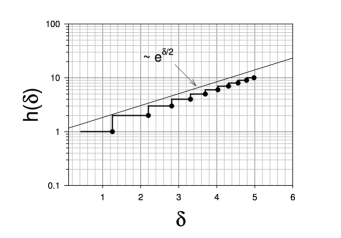
Figure 1: Equilibrium stripe width as a function of $\delta$ at $T=0$. Filled circles indicate the values of delta at which two adjacent striped configurations take the same energy.

At low but finite temperatures, the local magnetization inside the stripes decrease, i.e., $|m_{i}|<1$. Let us consider, for instance, a vertical striped state of width $h$. We demand the solutions of Eqs.(11) to satisfy the conditions: $m_{(x+h,y)}=-m_{(x,y)}$ $\forall x,y$ and $m_{(x,y)}=m_{(x,y^{\prime})}$ $\forall y,y^{\prime}$. This restricts the harmonics in Eq.(7) to those satisfying $(k_{x},k_{y})=(\pm(2l+1)\pi/h,0)$, with $l$ an integer such that $2l+1\leq h$. For instance, for $h=1$ we only have $k_{x}=\pi$; for $h=2$ we have $k_{x}=\pm\pi/2$; for $h=3$ we have $k_{x}=\pm\pi/3,\pi$; etc. In other words, for a stripe solution of width $h$ we have $h$ independent complex amplitudes $\hat{m}_{\vec{k}}$. In order to obtain pure real solutions we must impose $\hat{m}_{\vec{k}}^{*}=\hat{m}_{-\vec{k}}$. Replacing those conditions into Eqs.(7) and (11) leads to a set of $h$ non-linear algebraic equations for the amplitudes that can be solved numerically. To solve those equations we must evaluate $\hat{J}(k_{x},0)$ from Eq.(8). A suitable approximation for that function is (see Appendix A)

$$\hat{J}(k_{x},0)\approx 2\,\delta\,(\cos k_{x}+1)-k_{x}^{2}+2\pi|k_{x}|-\frac{2\pi^{2}}{3}-2\,\zeta(3)$$ (12)

where $\zeta(x)$ is the Riemann zeta-function. For the antiferromagnetic solution $m_{(x,y)}=m_{0}(-1)^{x+y}$ we have to compute

$$\hat{J}(\pi,\pi)=-4\,\delta+3\,\zeta(3)-4\,\sum_{x=1}^{\infty}(-1)^{x}\sum_{y=1}^{\infty}\frac{(-1)^{y}}{(x^{2}+y^{2})^{\frac{3}{2}}}$$ (13)

where the last term is calculated numerically. We calculated the MF stripe solutions for $h=1,\ldots,6$ for a wide range of values of $(\delta,T<T_{c})$. To discriminate whether they are actually minima we analyzed the second derivatives of the free energy. For every value of $h$ we first analyzed the stability of the solutions, that is, for every value of $\delta$ we calculated the temperature $T_{s}(\delta)$ above which non trivial solutions of the above described type cease to exist. This can be done by linearizing the corresponding set of equations around $\hat{m}_{\vec{k}}=0$ and demanding the condition of non–trivial solution, i.e., zero determinant of the linearized equations; this leads to the expression

$$T_{s}(\delta,h)=\hat{J}\left(\frac{\pi}{h},0\right)$$ (14)

The stability lines are shown in Fig.2, together with $T_{c}(\delta)$. It can be seen that for large values of $\delta$ the stability lines accumulate near the order-disorder transition line $T_{c}(\delta)$, implying an increasingly large number of metastable states as $\delta$ increases. Another remarkable fact, is the presence of regions near $T_{c}(\delta)$ where no striped solutions exists (see Fig.2). In those regions another type solutions appear, which are composed by parallel ferromagnetic stripes of different widths. We called them hybrid states. The hybrid states, which we denote by $<h_{1}^{n_{1}}\,h_{2}^{n_{2}}\,\ldots\,h_{l}^{n_{l}}>$, following the notation of Selke and Fisher Selke and Fisher (1979) for the axial next-nearest-neighbor Ising model (ANNNI), consists in the periodic repetition of a fundamental pattern composed by $n_{1}$ stripes of width $h_{1}$ (with opposite orientation), followed by $n_{2}$ stripes of width $h_{2}$ and so on. The regions where the hybrid states appear are shown in the MF phase diagram presented in Fig.3. The boundaries between ordered phases (corresponding to first order transitions) where determined by comparing the free energies of the different solutions (striped and hybrid) using Eq.5; they are shown by dashed lines in Fig.3. We found that the hybrid states appear through a sort of branching process near the boundary between two stable striped solutions as the temperature approaches $T_{c}$ from below. For instance, the transition line between the striped phases $h=1$ and $h=2$ ends in a triple point where a stable phase $<1\,2>$ appears between them; as we increase $\delta$ the transition line between the striped phase $h=2$ and the hybrid one $<1\,2>$ bifurcates in a new triple point giving rise to the appearance of a $<1\,2^{2}>$ phase between the $<1\,2>$ and the $h=2$ and so on (see inset of Fig.3). As the temperature increases more complicated hybrid states proliferate (we just show a few of them in Fig.3 as an example), in a completely analogous way as in a related model, namely, the three dimensional Ising model with competing short range ferromagnetic interactions and long range Coulomb interactionsGrousson et al. (2000). The MF phase diagram of that model is very similar to that of the present one, the striped states being replaced by lamellar ones.

Finally, we found evidences that the proliferation of hybrid states also happens near the boundary between striped phases with larger widths (for instance, 3 and 4), but they appear very close to $T_{c}$ and the computational effort needed to obtain an accurate estimation of the phase boundaries becomes very high.

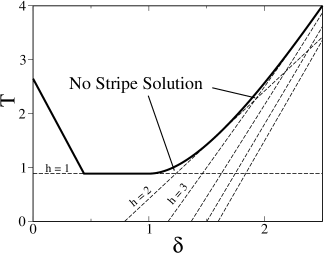
Figure 2: Stability lines $T_{s}(\delta,h)$ for the MF striped solutions at finite temperatures (dashed). Full line: critical temperature $T_{c}(\delta)$.

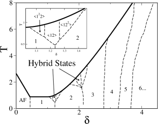
Figure 3: Mean field phase diagram. The numbers in the low temperature region indicate the equilibrium stripe width $h$ of the phases. Dashed lines correspond to first order phase transition between ordered phases,; the full line corresponds to the critical temperature $T_{c}(\delta)$. Inset: zoom of the hybrid region near the boundary between the striped phases $h=1$ and $h=2$.

III Monte Carlo phase diagram

Different parts of the phase diagram of this model were analyzed by different authors using MC numerical simulations, for small values of $\delta$ and small system sizesMacIsaac et al. (1995); Booth et al. (1995); Gleiser et al. (2002); Cannas et al. (2004b, 2006); Rastelli et al. (2006). In this section we extend those results to other parts of the phase diagram and to larger system sizes (in some cases), in order to obtain a complete description of the small-$\delta$ phase diagram that can be compared with the MF phase diagram.

The MC results were obtained using heat bath dynamics on $N=L\times L$ square lattices with periodic boundary conditions (Ewald sums were used to handle itDe’Bell et al. (2000)). We analyzed the equilibrium behavior of different quantities for system sizes running from $L=24$ to $L=84$; the maximum size used for each quantity were chosen according to the associated computational effort.

The first quantity we calculated was the order–disorder transition temperature as a function of $\delta$, which we called $T_{c}^{(2)}(\delta)$ (analog to $T_{c}(\delta)$ in the MF case). This quantity was determined by means of the specific heat

$$C(T)=\frac{1}{NT^{2}}\left(\left<H^{2}\right>-\left<H\right>^{2}\right)$$ (15)

where $\left<\cdots\right>$ stands for a thermal average. For some values of $\delta$ we also calculated the fourth order cumulant

$$V(T)=1-\frac{\left<H^{4}\right>}{3\left<H^{2}\right>^{2}}$$ (16)

to characterize the order of the phase transition.

At intermediate high temperatures (close to the order disorder transition and above it) this system presents a partially disordered phase with broken orientational order called tetragonal liquidBooth et al. (1995); De’Bell et al. (2000); Cannas et al. (2004b); Casartelli et al. (2004); Cannas et al. (2006). It is characterized by domains of stripes with mutually perpendicular orientations forming a kind of labyrinthine structure. At higher temperatures these domains collapse and the system crosses over continuously to a completely disordered phase (paramagnetic), without a sharp phase transition between themDe’Bell et al. (2000). While the existence of the tetragonal liquid phase has been clearly established by MC simulations, it is completely absent in the MF approximation (we discuss this point in section IV). MC simulations also showed recentlyCannas et al. (2006) that for $\delta=2$ an intermediate phase with nematic order is present between the tetragonal liquid and the striped phase. The nematic phase is characterized by positional disorder and long range orientational order and is consistent with one of the two possible scenarios predicted by a continuum approximation for ultrathin magnetic films in Refs.Kashuba and Pokrovsky (1993); Abanov et al. (1995). The presence of the nematic phase is reflected (among several manifestations) in the appearance of two distinct maxima at different temperatures in the specific heat, associated with the stripe–nematic and the nematic–tetragonal liquid phase transitions respectively. On the other hand, it was shown that for $\delta=1$ the specific heat present a unique maximum, consistent with a direct transition from the tetragonal liquid to the striped phaseCannas et al. (2006), suggesting that the nematic phase is only present for some range of values of $\delta$. We will call $T_{c}^{(2)}$ the temperature of the high temperature peak of the specific heat, whenever it presents two peaks, or the temperature of the unique peak if only one is present (for the system sizes considered and between the precision of the calculation). We will call $T_{c}^{(1)}$ the temperature of the low temperature peak of the specific heat, when it presents two peaks. While the calculation of $T_{c}^{(2)}$ is relatively easy, the calculation of $T_{c}^{(1)}$ is much more complicated and subtle, as it will be discussed below. $T_{c}^{(2)}$ was calculated for different values of $0\leq\delta\leq 4.2$ using the following simulation protocol: for each value of $\delta$ we let first the system thermalize at a high enough temperature (such that it is in the disordered phase) during $10^{5}$ Monte Carlo Steps (MS); after that, we calculated the specific heat for decreasing temperatures, down to a temperature well below the transition region. For every temperature we took the final configuration of the previous one and discarded the first $2\times 10^{4}$ MCS for thermalization and averaged over $10^{5}$ MCS. Every curve was averaged then over $40$ independent runs. This calculation was performed for system sizes $L\sim 50$ for all the values of $\delta$, in order to make the finite size bias comparable (for every value of $\delta$ we choose the closer value of $L$ commensurated with the modulation $2h$ of the corresponding ground state width). The results are shown by triangles joined by a continuous line in Fig.4. The order of the associated phase transition will be discussed in section IV.

We next calculated the stability of the striped phases in different parts of the phase diagram. It was shown in Ref.Gleiser et al. (2002) that the striped phases can remain in a meta-stable state for values of $\delta$ such that the equilibrium ground state width corresponds to a different stripe width. Following the same procedure as in Ref.Gleiser et al. (2002) we analyzed the striped staggered magnetization

$$m_{h}=\frac{1}{N}\left<\left|\sum_{x,y}\,(-1)^{f_{h}(x)}\,S_{x,y}\,\right|\right>$$ (17)

whereDe’Bell et al. (2000) $f_{h}(x)=(i-mod(x,h))/h$ and $x,y=1,\ldots,N$. This quantity takes the value one in a completely ordered vertical striped state of width $h$ and zero in a disordered state (paramagnetic, tetragonal or nematic). Starting from an initially ordered vertical striped state at zero temperature we increase the temperature up to high temperatures, averaging $m_{h}$ at every step and using a similar procedure as for the calculation on $T_{c}^{(2)}$, but averaging over $10^{6}$ MCS for every temperature to diminish metastability effects (see discussion below). We repeated this calculation for different values of $\delta$ for each value of $h$; for every value of $\delta$ the curve $m_{h}(T)$ was averaged over 25 independent runs. Typical curves $m_{h}(T)$ are shown in Fig.5 for different values of $h$ and $\delta$. From these curves we estimated the stability lines $T_{s}(\delta)$ (i.e., the temperature above which $m_{h}=0$) for $h=1,...,5$ and $0<\delta<4.1$. The stability lines are shown in Fig.4

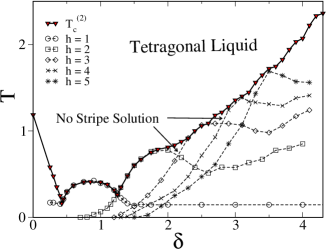
Figure 4: (Color on-line) Order-disorder transition temperature $T_{c}^{(2)}(\delta)$ and striped stability lines $T_{s}(\delta)$ for different values of $h$ (see text for details).

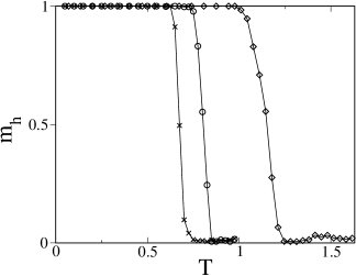
Figure 5: Staggered magnetization for different $\delta$ and $h$ values: $h=2$, $\delta=3.4$ and $L=60$ ($\times$); $h=3$, $\delta=4.1$, and $L=48$ ($\diamond$); $h=5$, $\delta=2.9$ and $L=40$ ($\circ$).

As in the MF case, we observe the existence of regions below $T_{c}^{(2)}$ where no stable striped solutions exist, at least up to $\delta=3$; for values of $\delta>3$ the data becomes very noisy (probably due to finite size effects) and the large error bars do not allow to identify clearly those regions for the present system sizes. We found that the equilibrium phase in those regions is a nematic one, instead of an hybrid state, as in the MF case (we checked the possible presence of hybrid states in those regions and they always decay after a short time into a nematic one). The nematic phase is characterized by an algebraic decay of the spatial spin-spin correlations in one of the coordinate directions and an exponential decay in the other. This can be study through the structure factor (Fourier transform of the correlation function):

$${\cal S}(\vec{k})\equiv\left\langle\left|\hat{S}_{\vec{k}}\right|^{2}\right\rangle$$ (18)

where $\hat{S}_{\vec{k}}=\frac{1}{N}\,\sum_{i}{S_{i}\,e^{-i\vec{k}\vec{r}_{i}}}$. Cannas et alCannas et al. (2006) calculated an approximate expression for the nematic phase structure factor:

$${\cal S}(\vec{k})\approx\frac{\delta_{k_{y},0}}{2\sqrt{N}}\,\left(\frac{\lambda}{(k_{x}-k_{0})^{2}+\lambda^{2}}+\frac{\lambda}{(k_{x}+k_{0})^{2}+\lambda^{2}}\right)$$ (19)

We ran simulations for $L=72$ and different $\delta$ values in the uncovered regions. The system was slowly heated from zero temperature using the same process described above, up to a temperature in the uncovered region, where we calculated ${\cal S}(\vec{k})$ by averaging over $2\times 10^{5}$ MCS. The typical observed behavior of ${\cal S}(\vec{k})$ is shown in Fig.6, together with Lorentzian fittings using Eq.(19); two typical spin configurations in corresponding regions can be seen in Fig.7 (compare with the results of Ref.Cannas et al. (2006)).

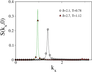
Figure 6: Structure factor for a $L=72$ system with $\delta=2.1,T=0.78$, ($\circ$) and $\delta=2.7,T=1.12$ ($\diamond$). Continuous lines correspond to fittings using (19): for $\delta=2.1,T=0.78$, we obtained $\lambda=0.033,k_{0}=1.39$, for $\delta=2.7,T=1.12$, $\lambda=0.0149,k_{0}=0.947$. $S(0,k_{y})=0$ $\forall k_{y}$ in both cases.

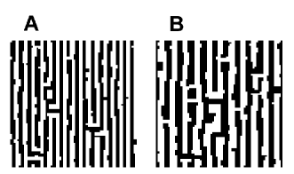
Figure 7: Typical nematic spin configurations for $L=72$. (A) $\delta=2.10$, $T=0.78$; (B) $\delta=2.70$, $T=1.12$.

Following the same steps as in the MF case, we calculated next the transition lines between different phases at low temperature. The transition lines were obtained by comparing the free energies of the striped phases of widths $h$ and $h+1$. The system size was chosen in these calculations to be a multiple of both $2h$ and $2(h+1)$. In what follows we will assume that the free energy of a meta–stable state can be obtained by following a thermodynamical path (that is, a close sequence of equilibrated states) from a thermodynamically stable reference state. To calculate the free energy of a striped phase of width $h$ we first computed the internal energy per spin $u(T,\delta_{i})\equiv\left<H\right>/N$ along a quasi-static path from an initially low temperature $T_{0}$ up to a working temperature $T<T_{s}(\delta_{i})$ keeping $\delta_{i}$ constant and taking the initial spin configuration of a given temperature as the final configuration of the previous one; the value of $\delta_{i}$ was chosen well separated from the border value at zero temperature between the striped phases of widths $h$ and $h+1$. The free energy was then obtained by numerically integrating the thermodynamic relation

$$\beta f_{h}(\beta,\delta_{i})=\beta_{0}\,f_{h}(\beta_{0},\delta_{i})+\int_{\beta_{0}}^{\beta}u(\beta^{\prime},\delta_{i})d\beta^{\prime},$$ (20)

where $\beta=1/T$ and $\beta_{0}=1/T_{0}$. Once we arrive to the final configuration at $(T,\delta_{i})$ we perform a second quasi-static path at constant temperature, by slowly changing $\delta$, up to a final value $\delta_{f}$ corresponding to a striped ground state of width $h+1$. Along this path we measure the average exchange energy

$$u_{ex}(\beta,\delta)\equiv-\frac{1}{N}\left<\sum_{<i,j>}S_{i}S_{j}\,\right>$$ (21)

From the expression

$$f=-\frac{1}{N\beta}\,\log{{\cal Z}}$$ (22)

where ${\cal Z}$ is the partition function, is easy to see that

$$\frac{\partial f}{\partial\delta} = u_{ex}(\beta,\delta).$$ (23)

Hence, the free energy along the last path can be obtained by numerically integrating the equation

$$f_{h}(\beta,\delta)=\int_{\delta_{i}}^{\delta}u_{ex}(\beta,\delta^{\prime})\,d\delta^{\prime}+f_{h}(\beta,\delta_{i})$$ (24)

Repeating the same procedure for the striped phase $h+1$, but following the second path in the inverse sense (i.e., decreasing $\delta$ from $\delta_{f}$ down to $\delta_{i}$) we calculated the free energy $f_{h+1}(\beta,\delta)$ at the same temperature. The transition point $\delta_{t}(T)$ is obtained from the equation $f_{h}(\beta,\delta_{t})=f_{h+1}(\beta,\delta_{t})$. We calculated the first order transition lines between striped phases up to $h=6$. The results are shown in the MC phase diagram of Fig.8 (the transition lines between the AF and the $h=1$ and between the $h=1$ and $h=2$ phases were already calculated in Ref.Gleiser et al. (2002); we put it here for completeness). Notice that all the calculated transition lines are almost independent of $T$, at variance with the MF prediction.

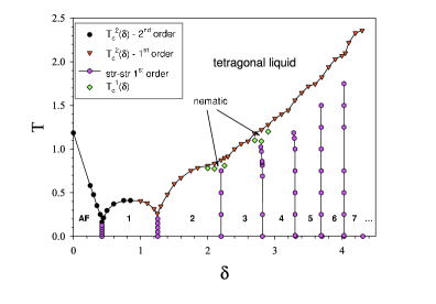
Figure 8: (Color on-line) Monte Carlo phase diagram. The numbers indicate the equilibrium width of the low temperature striped phases. The order of the different phase transition lines are indicated in the inset (see text for details). The continuous lines are a guide to the eye.

We next analyzed the transition temperature $T_{c}^{(1)}$ between the nematic and the striped phases. In order to check whether the stability lines $T_{s}(\delta)$ can be used to estimate $T_{c}^{(1)}$, we analyzed the behavior of the specific heat and fourth order cumulant Eqs.(15) and (16) around the regions below $T_{c}^{(2)}$ where no striped states exist. The simulation protocol used to determine $T_{c}^{(2)}$ is completely unable to detect the low temperature transition at $T_{c}^{(1)}$. This is because free energy barriers associated with both transitions for the system sizes here considered are larger around $T_{c}^{(1)}$ than around $T_{c}^{(2)}$, as was shown in Ref.Cannas et al. (2006). Indeed, a rough estimation of the average times needed by the system to jump the free energy barrier between the striped and the nematic phases are of the order of the millions of MC, thus generating a strong meta-stability when the average times are of the order of $10^{5}$ MCSCaM . In Ref.Cannas et al. (2006) it was shown that an accurate estimation of $T_{c}^{(1)}$ for $\delta=2$ requires, for every temperature, average times of the order of $2\times 10^{8}$ MCS. However, we verified that an average time of $5\times 10^{7}$ is enough to determine $T_{c}^{(1)}$ between the error bars we are using in the present calculation (although such time scales are not enough to determine the height of the specific heat maximum with precision and therefore to allow a finite size scaling analysis). In order to save computational effort, we used the following procedure for fixed values of $\delta$ around the regions of interest: first we ran the same simulation protocol as for $T_{c}^{(2)}$ down to low temperatures and repeated it for the same parameter values, but heating from a low temperature up to high temperatures and taking as initial configuration the ordered striped state. In both cases we calculated the internal energy $u(T)$ along the path. This allowed us to determine the approximated location of $T_{c}^{(1)}$, by looking at the temperature range where the internal energy exhibit meta-stabilityCaM . Then we calculated $C$ and $V$ for a limited set of temperatures in that region, by taking averages for each temperature over a single MC run of $5\times 10^{7}$ MCS. In order to get a more accurate estimation of $T_{c}^{(2)}$ for the same values of $\delta$ we also repeated the latter calculation for temperatures around the previous estimation of $T_{c}^{(2)}$ taking averages over $10^{7}$ MCS. These calculations were performed for $\delta=2.1$ and $2.25$ (near the $h=1-h=2$ border with $L=48$. The behavior of $C$ and $V$ for $\delta=2.25$ is shown in Fig.9 (compare with the results of Ref.Cannas et al. (2006)). We verified that the location of the low temperature peak of $C$ coincides between the error bars with the value of $T_{s}(\delta)$ for the same values of $\delta$. The values of $T_{c}^{(1)}$ for $\delta=2$ (from Ref.Cannas et al. (2006)), $\delta=2.1,\,2.25$ (from the above calculation) and $\delta=2.7,\,2.8,\,2.9$ (estimated from the stability lines) are shown by diamonds in the MC phase diagram of Fig.8. Reliable calculations of $T_{c}^{(1)}$ for larger values of $\delta$ would require system sizes that are out of the present computational capabilities.

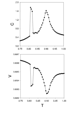
Figure 9: Specific heat and fourth order cumulant as a function of $T$ for $\delta=2.25$ and $L=48$.

IV Discussion

We have presented a detailed calculation of the finite temperature phase diagram of the Ising dipolar model in the range $0\leq\delta\leq 4$, which allow striped ground state configurations of width up to $h=7$. We compared the predictions of MF approximation with extensive MC numerical simulations. Although the overall appearance of both phase diagrams looks similar, several differences are remarkable.

The first difference to be noticed is the absence of nematic and tetragonal order in the MF approximation. This results from the fact that both phases are spatially disordered, which implies that $\left\langle\hat{S}_{\vec{k}}\right\rangle=\hat{m}_{\vec{k}}=0$ $\forall\vec{k}$. The characteristic features of those states, namely, the broken rotational symmetry of the nematic state and the discrete rotational symmetry of the tetragonal state can only be observed when looking at the behavior of the spatial correlations, or equivalently, of the structure factorDe’Bell et al. (2000); Cannas et al. (2006) Eq.(19). Since fluctuations are neglected in the MF approximation it follows that ${\cal S}(\vec{k})=\hat{m}_{\vec{k}}\hat{m}_{-\vec{k}}=0$ and therefore the only possible spatially disordered solution within this approximation is the paramagnetic one. On the other hand, the MF approximation presents hybrid states solutions in the regions of the phase diagram where MC predicts only nematic order. Moreover, we verified that hybrid states are unstable in that regions, suggesting that (in the language of renormalization group) fluctuations play the role of a relevant scaling field that turns the MF hybrid fixed points unstable towards nematic attractors (in some sense, the hybrid states could be the closest state to a nematic one that can obtained when fluctuations are neglected). This would be consistent with the fact that fluctuations, when included, can modify the continuous nature MF prediction for the phase transition between the high temperature disordered phase and the low temperature ordered one: Hartree approximation applied to the continuous version of Hamiltonian (1) predicts a fluctuation induced first order transition any finite value of $\delta$ Cannas et al. (2004b), which continuously fades out for increasing values of $\delta$ CaM . In fact, MC simulations show a more complex scenario, where the nature of the order–disorder phase transition at $T_{c}^{(2)}$ depends on the value of $\delta$.

Rastelli et al have shown that for $\delta=0$ the transition is indeed continuous and belongs to the universality class of the nearest neighbors Ising modelRastelli et al. (2006). They also found a rather clear evidence of a second order transition for $\delta=0.85$, but with an unusual value for the critical exponent $\beta$Rastelli et al. (2006). However, Cannas et al have shown that for $\delta=1$ the system presents a weak first order phase transitionCannas et al. (2006). These results are consistent with the presence of a second order transition line for small values of $\delta$, that joins with continuous slope a first order transition line for larger values of $\delta$ at a tricritical point somewhere between $\delta=0.85$ and $\delta=1$ and the unusual critical exponents at $\delta=0.85$ is probably due to a crossover effect near the tricritical point. There are also clear evidences that the transition is first order for $\delta=2$ (Refs.Cannas et al. (2004b, 2006)) and $\delta=1.7,2.5$ (Ref.Rastelli et al. (2006)). The behavior of the fourth order cumulant observed in the present work for $\delta=2.1$ and $\delta=2.25$ is also consistent with a first order transition. For $\delta=3$ the results of Rastelli et alRastelli et al. (2006) appear to suggest that the transition becomes continuous again. However, this is a matter of debateCaM and numerical results using a completely different techniqueCasartelli et al. (2004) for $\delta=4.45$ are also consistent with a first order transition.

We also presented numerical evidences of the presence of an intermediate nematic phase between the disordered and the striped ones in different parts of the phase diagram. Although it seems that the nematic phase is only located near the border lines between striped states, the presence of this phase in other regions in narrow ranges of temperatures cannot be excluded and larger system sizes should be required to clarify this.

The existence of both type of scenarios for relatively large values of $\delta$, namely one direct first order transition from the striped phase to the tetragonal liquid or two phase transitions with an intermediate nematic phase would be in qualitative agreement with theoretical predictions based on a continuous approachKashuba and Pokrovsky (1993); Abanov et al. (1995). It is worth mention that Abanov et alAbanov et al. (1995) conjectured a second order nematic-tetragonal phase transition; since their whole analysis is based on mean field arguments, the disagreement with the MC results can be understood from the fluctuation-induced nature of the transition (see the discussion in Refs.Cannas et al. (2004b, 2006)). Regarding the order of the transition at $T_{c}^{(1)}(\delta)$, the situation is less clear. Cannas et alCannas et al. (2006) have shown for $\delta=2$ that, even the finite size scaling is consistent with a first order transition, the energy changes continuously at $T_{c}^{(1)}(\delta)$ in the thermodynamic limit; this produces a saturation in the associated specific heat peak, behavior that strongly resembles that observed in a Kosterlitz-Thouless transition. That could be indicative of the emergency of smectic order between the nematic and the striped phases for larger system sizes and would be in qualitative agreement with theoretical predictions based on a continuous approachKashuba and Pokrovsky (1993); Abanov et al. (1995). If that would be the case, probably our calculation of $T_{c}^{(1)}(\delta)$ overestimates the true transition temperature, since it is known that the specific heat peak locates above the KT transition temperatureChaikin and Lubensky (1995), and therefore the nematic phase would extend in larger regions of the phase diagram. However, at the present level it is very difficult to improve this estimation due to finite size effects.

Regarding the low temperature behavior, a remarkable prediction of both MF and MC is the existence of an increasingly large number of striped meta-stable states as $\delta$ increases.

Finally, we found that, at variance with the MF prediction, up to $\delta=4$ the transition lines between striped phases are completely vertical, imply temperature independence of the stripe width. This suggests the existence of some large threshold value of $\delta$, above which wall fluctuations makes the system to cross over to a "mean field regime", where it starts to exhibit temperature dependency of the stripe width.

Fruitful discussions with D. A. Stariolo, F. A. Tamarit, P. M. Gleiser, D. Pescia, A. Vindigni and O. Portmann are acknowledged. This work was partially supported by grants from CONICET (Argentina), SeCyT, Universidad Nacional de Córdoba (Argentina) and ICTP grant NET-61 (Italy).

Appendix A

When $k_{y}=0$ Eq.(8) can be written as

$$\hat{J}(k_{x},0)=2\,\delta(\cos{k_{x}}+1)-S(k_{x},0)$$ (25)

with

$$S(k_{x},0)\equiv\sum_{i}\frac{1}{r_{ij}^{3}}\cos{(k_{x}x_{i})}$$ (26)

where $x_{i}$ is the $x$ component of $\vec{r}_{i}$. This last term can be rewritten as follows:

$$S(k_{x},0)=2\sum_{x=1}^{\infty}\,\cos{(k_{x}x)}\>R(x)+2\,\zeta(3)$$ (27)

with

$$R(x)\equiv\sum_{y=-\infty}^{\infty}\frac{1}{{(x^{2}+y^{2})^{\frac{3}{2}}}}$$ (28)

$$\zeta(3) \equiv \sum_{y=1}^{\infty}\frac{1}{y^{3}}\approx 1.202$$ (29)

where $x,y$ represents the Cartesian coordinates of each site and $\zeta(x)$ is the Riemann zeta-function. $R(x)$ can be approximated byCzech and Villain (1989)

$$R(x)\approx\int_{-\infty}^{\infty}\frac{dy}{{(x^{2}+y^{2})^{\frac{3}{2}}}}=\frac{2}{x^{2}}$$ (30)

which has an error of $\%1$ in the worst case $(x=1)$. Inserting this in (27) we get

$$S(k_{x},0) \approx 4\sum_{x=1}^{\infty}\frac{\cos{(k_{x}x)}}{x^{2}}+\,2\,\zeta(3)$$ (31)

$$= k_{x}^{2}-2\pi|k_{x}|+\frac{2\pi^{2}}{3}+2\,\zeta(3)$$

which replaced in Eq.(25) gives the expression (12).

References

- Allenspach et al. (1990) R. Allenspach, M. Stampanoni, and A. Bischof, Phys. Rev. Lett. 65, 3344 (1990).
- Vaterlaus et al. (2000) A. Vaterlaus, C. Stamm, U. Maier, M. G. Pini, P. Politi, and D. Pescia, Phys. Rev. Lett. 84, 2247 (2000).
- De’Bell et al. (2000) K. De’Bell, A. B. MacIsaac, and J. P. Whitehead, Rev. Mod. Phys. 72, 225 (2000).
- Politi (1998) P. Politi, Comments Cond. Matter Phys. 18, 191 (1998).
- Portmann et al. (2003) O. Portmann, A. Vaterlaus, and D. Pescia, Nature 422, 701 (2003).
- Czech and Villain (1989) R. Czech and J. Villain, J. Phys. : Condensed Matter 1, 619 (1989).
- MacIsaac et al. (1995) A. B. MacIsaac, J. P. Whitehead, M. C. Robinson, and K. De’Bell, Phys. Rev. B 51, 16033 (1995).
- Booth et al. (1995) I. Booth, A. B. MacIsaac, J. P. Whitehead, and K. De’Bell, Phys. Rev. Lett. 75, 950 (1995).
- Stoycheva and Singer (2000) A. D. Stoycheva and S. J. Singer, Phys. Rev. Lett. 84, 4657 (2000).
- Gleiser et al. (2002) P. M. Gleiser, F. A. Tamarit, and S. A. Cannas, Physica D 168-169, 73 (2002).
- Cannas et al. (2004a) S. A. Cannas, P. M. Gleiser, and F. A. Tamarit, Two dimensional Ising model with long-range competing interactions (Transworld Research Network, India, 2004a), vol. 5 (II) of Recent Research Developments in Physics, pp. 751–780.
- Cannas et al. (2004b) S. A. Cannas, D. A. Stariolo, and F. A. Tamarit, Phys. Rev. B 69, 092409 (2004b).
- Casartelli et al. (2004) M. Casartelli, L. Dall’Asta, E. Rastelli, and S. Regina, J. Phys. A: Math. Gen. 37, 11731 (2004).
- Cannas et al. (2006) S. A. Cannas, M. F. Michelon, D. A. Stariolo, and F. A. Tamarit, Phys. Rev. B 73, 184425 (2006).
- Rastelli et al. (2006) E. Rastelli, S. Regina, and A. Tassi, Phys. Rev. B 73, 144418 (2006).
- Portmann et al. (2006) O. Portmann, A. Vaterlaus, and D. Pescia, Phys. Rev. Lett. 96, 047212 (2006).
- Won et al. (2005) C. Won, Y. Z. Wu, J. Choi, W. Kim, A. Scholl, A. Doran, T. Owens, J. Wu, X. F. Jin, and Z. Q. Qiu, Phys. Rev. B 71, 224429 (2005).
- Yafet and Gyorgy (1988) Y. Yafet and E. M. Gyorgy, Phys. Rev. B 38, 9145 (1988).
- Chaikin and Lubensky (1995) P. M. Chaikin and T. C. Lubensky, Principles of Condensed Matter Physics (Cambridge University Press, 1995), 1st ed.
- Selke and Fisher (1979) W. Selke and M. E. Fisher, Phys. Rev. B 20, 257 (1979).
- Grousson et al. (2000) M. Grousson, G. Tarjus, and P. Viot, Phys. Rev. E 62, 7781 (2000).
- Kashuba and Pokrovsky (1993) A. B. Kashuba and V. L. Pokrovsky, Phys. Rev. B 48, 10335 (1993).
- Abanov et al. (1995) A. Abanov, V. Kalatsky, V. L. Pokrovsky, and W. M. Saslow, Phys. Rev. B 51, 1023 (1995).
- (24) S. A. Cannas and M. F. Michelon and D. A. Stariolo and F. A. Tamarit, cond-mat/0701039.