Energy levels and their correlations in quasicrystals

Abstract

Quasicrystals can be considered, from the point of view of their electronic properties, as being intermediate between metals and insulators. For example, experiments show that quasicrystalline alloys such as AlCuFe or AlPdMn have conductivities far smaller than those of the metals that these alloys are composed from. Wave functions in a quasicrystal are typically intermediate in character between the extended states of a crystal and the exponentially localized states in the insulating phase, and this is also reflected in the energy spectrum and the density of states. In the theoretical studies we consider in this review, the quasicrystals are described by a pure hopping tight binding model on simple tilings. We focus on spectral properties, which we compare with those of other complex systems, in particular, the Anderson model of a disordered metal. We discuss “strong” and “weak” quasicrystals, which are described by different universal laws. We find similarities and universal behavior, but also significant differences between quasiperiodic models and models with disorder. Like weakly disordered metals, the quasicrystal can be described by the universal level statistics that can be derived from random matrix theory. These level statistics are only one aspect of the energy spectrum, whose very large fluctuations can also be described by a level spacing distribution that is log-normal. An analysis of spectral rigidity shows that electrons diffuse with a bigger exponent (super-diffusion) than in a disordered metal. Adding disorder attenuates the singular properties of the perfect quasicrystal, and leads to improved transport. Spectral properties are also used in computing conductances of such systems, and to attempt to resolve the experimental enigmas such as whether quasicrystals are intrinsically conductors, and if so, how conductances depend on the structure.

I I. Introduction

Inside a perfect quasicrystal, such as the Penrose tiling penrose or the octagonal tiling shown in Fig.1, a freely wandering observer would find a small reoccurring set of local environments, as in crystals. The sequence of environments, however, does not repeat periodically, in the case of the quasicrystal. The repetitivity property states that any given pattern is guaranteed to be repeated within a distance proportional to the linear size $R$ of the pattern. Random structures are very different in this respect, in that the number of patterns increases rapidly with the size of the pattern, and in this case identical regions of size $R$ will be typically separated by distances that are exponentially large for large $R$. This geometric property has implications for the spatial extent of wavefunctions, as we will see later. Since the repetition is not periodic, one does not have a Bloch theorem in the quasicrystal. That the quasiperiodic structure is not random is perhaps best seen by calculating its structure factor, which turns out to have sharp Bragg peaks, as in a crystal levine . The structure factor of a quasicrystal can also exhibit 5-fold 8-fold or 10-fold symmetries that are forbidden for crystals.

A wave packet representing an electron that enters such a quasiperiodic medium will be scattered by the quasiperiodic potential, giving rise to a complex superposition of wave vectors and corresponding phase shifts. What does a typical wavefunction look like, and what are the allowed energy levels ? Would the electrons conduct an electrical current, and if so, what factors determine the value of the conductivity in a real quasicrystal ? Such questions have been asked, since the discovery by Schechtman et al shecht of real quasicrystals in 1984. Some answers have been provided, by direct experimental measurement, and in numerical calculations. However, many basic questions concerning the properties of even the simplest two-dimensional quasiperiodic structures remain unanswered.

Figure 1: Finite piece of a quasiperiodic structure

In this paper we present a review of some electronic properties of a single electron in a quasiperiodic solid in two dimensions. This is the lowest dimension in which new physics due to the interplay between order and disorder is expected to arise. A well known example is that of disordered crystalline solids described by the Anderson model anderson , where any disorder, no matter how weak, “wins out” over the periodic order and exponentially localizes wavefunctions, in one dimension. In two dimensions, this tendency is less marked, and one has the notion of weakly and strongly localized wavefunctions. A transition between localized-delocalized transition only occurs, in the Anderson model, in three dimensions and above. A similar situation could be expected to hold for the quasiperiodic Hamiltonians. The case of one dimension is the most tractable, in that analytical methods can be combined with numerical solutions in order to get a good appreciation of the expected physics. However, once again, one dimension is special in that the quasiperiodic potential is almost always a relevant variable (in the sense of the renormalization group).

One of the principal symmetries of the quasicrystal is its invariance under a scale change – inflations and deflations (to be described in Sec.II). The scale invariance of quasiperiodic structures, and in consequence, the potential seen by the electrons, must play an important role in determining the spatial dependence and the energy of the eigenstates. The characteristic singular features in the density of states and other electronic properties are in fact a result of this symmetry. There have been attempts to exploit the heirarchical symmetry of the tiling in order to obtain renormalization equations siremoss1 for tight-binding models, but the method breaks down for the pure hopping models that we discuss here. In a different context, another RG scheme was introduced for a spin model on this tiling, in order to calculate ground state energy and local magnetizations jag1 . It is therefore necessary, in the absence of analytical tools, to take a numerical approach to the electronic problem.

Tilings can be deterministic (“perfect”) or random. It is of interest to study the effects of including geometric disorder since real quasicrystals may well be intrinsically disordered in this sense. Random tiling models have been introduced (see review in henley ) as the basic templates for naturally occurring quasicrystals. In contrast to the perfect tiling, the random tiling has a lower free energy due to the associated entropy, explaining why materials might choose to condense with this type of long range order. Careful X-ray diffraction experiments must be done boissieu to distinguish the random tiling from the perfect tiling, as Bragg peaks occur in the same positions - this shows that the geometrical constraints are locally strong enough to ensure that even in random tilings the structure retains long range order with an infinite correlation length.

The experimental motivation for our studies comes from a large number of intriguing results for the electrical conductivity of quasicrystals. Firstly, the low temperature electrical conductivity of quasicrystals is anomalously low, many orders of magnitude smaller than that of its constituent metals, aluminium, zinc, copper or iron, etc. Secondly, the conductivity rises with temperature, contrarily to the usual metallic behavior. Thirdly, when the structural disorder initially present in as-quenched samples of AlFeCu is removed by annealing, the conductivity gets smaller klein . Similarly, in samples of AlPdMn prepared by different methods, the sample of higher structural perfection has the lower conductivity swen ; pre . Disorder appears to facilitate transport in the quasicrystal, contrarily to its effect in disordered metals. Finally, studies of complex alloy system for the AlPdMn with very large unit cells show that the conductivity was higher for these than for a single grain quasicrystal of similar composition, although both alloys had comparable structural quality. This could indicate that the transport is not just determined by local properties, but also by the long range quasiperiodic structural order.

Many phenomenological mayou and numerical fuji studies have therefore addressed the problem of explaining the magnitude and temperature dependence of the electrical conductivity in realistic models. However studies of even the simplest of tight binding models show that the properties of the quasicrystal are far more complex than those of crystals. Therefore, our focus in this paper is restricted to the simplest of two dimensional quasiperiodic tilings and determining for these whether states are expected to be localized or extended, whether electrons will conduct, and how best to describe the complex dynamics in such systems.

II I. Definitions and general background

We consider tight-binding Hamiltonians of the form

$$H=-\sum_{\langle i,j\rangle}t_{i}(c^{\dagger}_{i}c_{j}+c^{\dagger}_{j}c_{i})+\sum V_{i}c_{i}^{\dagger}c_{i}$$ (1)

in terms of onsite electron creation and annihilation operators $c_{i}^{\dagger}$ and $c_{i}$ on a variety of two dimensional structures. The first term allows for hopping between connected sites with amplitudes $\{t_{i}\}$, while the second term allows for variations in the onsite potential. Although this Hamiltonian is grossly oversimplified, it contains the essential information about the quasiperiodic structure, namely, its geometry. For a discussion of the tight-binding Hamiltonian and its properties, particularly for one-dimensional quasicrystals, the reader is referred to sire . In two dimensions, there have been many calculations for this type of model and its dual version on the octagonal (Ammann-Beenker) and the Penrose tilings oda ; koh ; suth2 ; kumar ; toki ; benza1 ; benza2 ; jag2 ; pj ; zhong ; zijl ; tsune ; tsune2 .

We will now simplify the Hamiltonian even further by setting henceforth all of the hopping amplitudes equal to a constant, $t=1$, and all the $V_{i}=0$. This is because we wish to focus exclusively on the effects of the quasiperiodic connectivity between atoms. Any variations in the hopping amplitude, or of the local potentials has the effect of accentuating the quasiperiodic modulation and opening gaps in the spectrum. For example, if one includes onsite potentials $V(\bf{r}_{i})$ that are proportional to the site coordination number, one gets, even for moderate values of $V$, bands separated by true gaps, and wavefunctions which have a quasi one-dimensional character benza1 ; zijlstra .

The Anderson model for disordered conductors belongs in this class of tight-binding Hamiltonians. The disorder is realized by taking random hopping amplitudes and/or random onsite potentials or both. Such models are used, for example, to study critical properties at the metal-insulator transition in three dimensions. Spectral statistics in the Anderson model have also been discussed intensively, and compared with those of other classically chaotic systems. These studies ( see for example the review in andersonrefs ), along with the predictions of random matrix theory provide the background for the present discussion of the quasicrystal.

II.1 Obtaining planar quasiperiodic structures

A standard method of obtaining quasicrystals and their approximants consists of projecting down from a higher dimensional cubic lattice levine . A subset of points belonging to an infinite strip of this hypercubic lattice is projected onto the physical plane. Fig.2 (taken from durandref ) shows the projection onto the plane of a portion of the simple cubic lattice when the projection is rational (left-hand figure), and for an irrational orientation (right figure) where the structure never repeats. In these figures, the different faces of the hypercube are projected onto tiles of different colors. A similar approach can be used to obtain the Penrose (projection from five dimensions), the octagonal tiling (projection from four dimensions) and the weakly quasiperiodic tiling described in Sec. III (projection of the simple cubic lattice).

In calculations, the structures considered are often finite periodic samples, called periodic approximants, obtained by rational cuts in the hyperspace. The unit cell of N sites can be made arbitrarily large, by modifying the plane of projection. The use of approximants has the advantage of eliminating surfaces and thus spurious energy levels – at the price of introducing a few defects in the structure. However, these are of diminishing importance as the approximant size is increased, and the true quasicrystal structure is approached. For the square approximants of the octagonal tiling, we assume boundary conditions $\psi(x+L,y)=e^{ik_{x}L}\psi(x,y)$; $\psi(x,y+L)=e^{ik_{y}L}\psi(x,y)$ where $k_{\mu}=2\pi n_{\mu}/L$ and $L$ is the repeat length of the approximant in each direction. An arbitrary external magnetic flux through a gauge field $\phi$, can also be introduced by suitably modifying the hopping amplitudes by a phase factor. As we will see, the addition of magnetic flux changes the symmetry properties of the Hamiltonian, with a corresponding change in spectral characteristics.

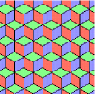
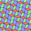
Figure 2: a)a periodic projection and b) an aperiodic projection of the cubic lattice

The $N\times N$ real symmetric matrix representing $H$ is numerically diagonalized for each $\{k_{x},k_{y}\}$ and the set of eigenvalues is used to compute the density of states and interesting statistical properties of energy levels. For purposes of computing the density of states, assuming large enough systems, it is in fact sufficient to compute the energy spectrum at $\vec{k}=0$. The two main statistical quantities considered are the nearest neighbor level spacing distribution $P(s)$ and the level rigidity function $\Sigma^{2}(E)$. These quantities are introduced now, along with some known results and their interpretation.

II.2 Level spacing statistics

After ordering the energy levels corresponding to a given $\vec{k}$ and parity, we can compute the set of spacings $s_{n}=E_{n+1}-E_{n}$. The mean level spacing is denoted by $\Delta$.

If the density of states $\rho(E)=N^{-1}\sum_{n}\delta(E-E_{n})$ were constant as a function of the energy, one would simply go on to construct the histogram representing the probability distribution $P(s)$ defined by Eq.4. However, in general, the density of states $does$ depend on the energy. In this case, the spacings must be redefined or “unfolded” so as to eliminate this trivial dependence on the position of the levels in the band. A systematic way to redefine spacings consists of fitting the integrated density of states by a smoothed “classical” part. This smoothed curve is then used to define a set of unfolded spacings (see boh ). $P({s})$ is now determined from the set of unfolded spacings $\{s_{n}\}$ using

$$P({s})=\frac{1}{N}\sum_{n=1}^{N}\delta({s}-{s}_{n})$$ (2)

The issue of the statistical analysis of energy levels was raised first for the spectra of large nuclei. The first theoretical calculations of level spacing distribution in complex systems were carried out by Wigner and by Dyson, for random matrices having independently distributed gaussian random matrix elements. The result depends on the class of matrix mehta . Three cases were distinguished: real symmetric matrices (gaussian orthogonal ensemble or GOE), complex unitary matrices (gaussian unitary ensemble or GUE) and, finally, symplectic random matrices (GSE)

$$P_{WD}(s)=A_{\beta}s^{\beta}{e}^{-C_{\beta}s^{2}}$$ (3)

where $\beta=1,2,4$ for GOE , GUE and GSE respectively. Values for the constants are, in the GOE case, $A_{1}=\pi/2$ and $C_{1}=\pi/4$. These distributions are written for spacings that have been normalized so that the mean level spacing $\Delta=1$. An impressive array of complex systems turn out to conform to one of these three expressions of $P_{WD}(s)$: heavy nuclei, chaotic billiards, correlated fermions in regular crystals, etc. The Wigner-Dyson distributions thus appear to be a universal feature of classically non-integrable systems where the motion is ergodic.

For the Anderson model, in the metallic regime many studies have confirmed that the level spacings obey GOE statistics. If time reversal symmetry is broken, by adding an external magnetic field, or by including a magnetic flux then GUE statistics are found. The third class of problems with $\beta=4$ has also been realized in metals containing spin-orbit scatterers.

Figure 3: Examples of spectra a) Uncorrelated energy levels b) disordered metal energy levels c) octagonal tiling energy levels

A feature of note in the level spacing distributions $P_{WD}$ is the fact that they tend to 0 as $s\rightarrow 0$. This expresses the unlikelihood of levels being degenerate in this system - the phenomenon of so-called level repulsion. Level repulsion occurs when electron wavefunctions are extended in the available volume, and when there is, in consequence, a non-negligible spatial overlap between states. In systems where wavefunctions are strongly localized, on the contrary, states in different regions of the sample do not overlap, and spatial correlations are negligible, there is no bar to two different states having the same energy. This is the reason that a discrete level spectrum corresponding to an insulator can be distinguished visually from that of of a weakly disordered metal. In Fig.3 three different kinds of spectra are illustrated (energies have been scaled so that there is the same mean spacing between levels for all three examples). In the insulator (left hand figure), distances between the energy levels of the insulator fluctuate greatly, and levels can approach arbitrarily close to each other. The middle figure represents energy levels of a disordered metal and was obtained by diagonalizing the Anderson model Hamiltonian. Here, levels repel each other due to non-negligible wavefunction overlap, and so there are fewer very small or very large spacings. Finally, the quasicrystal spectrum is intermediate between the first two examples (right hand figure).

Other probability distributions can be found in the literature, corresponding to other physically interesting problems. In cases where the classical dynamics of the electron is integrable, such as the motion of electrons in a crystal, the probability distribution of the set of all spacings is governed by a different law, the Poisson distribution,

$$P_{P}(s)={e}^{-s}$$ (4)

This behavior is found, as the name indicates, whenever the levels are randomly distributed according to a Poisson probability (the left hand figure in Fig.3). It is the level spacing distribution in the strong localization regime of the Anderson model. At the critical point of the metal-insulator transition, there have been proposals shklov for another form of $P(s)$ which is a hybrid between the exponential dependence at large $s$ of $P_{P}$ and the small $s$ level repulsion of $P_{WD}$: written above:

$$P_{c}(s)=A_{\beta}s^{\beta}\exp({-as^{(2-\gamma)}}$$ (5)

where $\beta$ has the values 1 or 2 or 4 as mentioned earlier.

The semi-Poisson distribution $P_{sp}$ is a special case of this type of law, with $\beta=\gamma=1$. The name semi-Poisson comes from the fact that this is the distribution for the distances between the midpoints between levels given a set of randomly chosen energy levels. There is level repulsion, but then the probability rises to a maximum and decays exponentially, as in the Poisson distribution. At the critical point, wavefunctions are expected to have multifractal character. This type of wavefunction leads to level repulsion, unlike states in the localized regime, but the effect is not as strong as that in the metallic regime.and Such multicritical wavefunctions have been linked to the level statistics at the critical point of the Anderson model chalker . This type of law has been observed to hold in the Anderson model if one averages the distribution over all boundary conditions kravt ; evan1 ; braun ; batsc , at the critical point of the Harper model evan2 and in a disordered two particle Hubbard model waintal . Another example with such statistics are the pseudointegrable billiards, studied by Bogomolny et al bogo .

II.3 The spectral rigidity function

As we mentioned in the last section, the system of energy levels displays a certain amount of rigidity. One measure of this rigidity is given by the variance of the number of levels in an energy interval of width $E$:

$$\Sigma^{2}(E)=\langle(N(E)-\langle N(E)\rangle)^{2}\rangle$$ (6)

where $N(E)$ is the total number of levels within an interval of width $E$. The average is taken over all positions of $E$ in the spectrum. In random matrix theory, the rigidity has been calculated to be a relatively slowly increasing function of $E$, with

$$\Sigma^{2}_{RMT}(E)=\frac{1}{\beta\pi^{2}}\ln(2\pi E/\Delta)$$ (7)

In comparison, the rigidity of a completely random set of levels, where the $P(s)$ is Poissonian, one has a linear dependence

$$\Sigma^{2}_{P}(E)=E$$ (8)

At the critical point, the spectral rigidities are also linear for small $E$, but with a smaller slope $\Sigma^{2}\sim\chi E$ ($\chi<1$), since correlations between levels begin to kick in, and lead to level repulsion. The semi-Poisson form will be described in more detail in the third section, for the case of the weakly quasiperiodic tiling.

The spectral rigidity function can be obtained from the two-level correlation function $K(E^{\prime})$ defined by $K(E^{\prime})=\langle N(E)N(E+E^{\prime})\rangle/\langle N(E)\rangle^{2}-1$. One can check that $\Sigma^{2}(E)=2\int_{0}^{E}dE^{\prime}(E-E^{\prime})K(E^{\prime})$. Argaman et al arga established a connection between the dynamics of an electron moving in the medium and the spectral form factor $K$. Adapting their calculations to a situation where an electron diffuses with an exponent $\sigma$ defined in terms of the root mean square distance $d$ explored in a time $t$ by $d\sim t^{\sigma}$, then the probability of return to the origin scales as $p(t)\sim t^{1-d\sigma}$ where $d$ is the spatial dimension. It can be shown (see for example akkmont ) that $p(t)$ is proportional to $K(t)/t$ where $K(t)=\frac{1}{2\pi}\int K(\omega)e^{-i\omega t}d\omega$. Transforming back to energy variables the power law in time for $K$ becomes a power law in the energy for $\Sigma^{2}$,

$$\Sigma^{2}(E)\sim E^{d\sigma}$$ (9)

Thus, if the rigidity function does indeed follow such a power law, one can from it deduce the exponent $\sigma$ describing quantum diffusion in the medium. For disordered metals, one has normal diffusion, $\sigma=\frac{1}{2}$, whereas as we will see, the motion in the quasicrystal is superdiffusive and $\sigma>\frac{1}{2}$.

In numerical calculations on disordered metals one usually finds different regimes of behavior of the spectral rigidity depending on the energy. The crossover energy scale between low and high energies is given by the Thouless energy, $E_{Th}=\hbar/t_{L}$, where $t_{L}$ is the time taken for the electron to diffuse to the boundary of the sample. This time depends on the diffusion exponent via $t_{L}\sim L^{1/\sigma}$. For small energies $E<<E_{Th}$, the behavior of $\Sigma^{2}$ is governed by the long time dynamics, which is completely ergodic since the electron has reached the boundary a large number of times. At such energies, the RMT logarithmic dependence is thus expected. For $E>>E_{Th}$, however, one expects to find a power law dependence, corresponding to the diffusive electron motion at times shorter than $t_{L}$.

II.4 Wavefunctions and quantum diffusion

The wavefunctions of the tight-binding Hamiltonian 1 are solutions of $H\psi^{(n)}=E_{n}\psi^{(n)}$. The set of amplitudes $\psi_{i}^{(n)}$ ($i=1,N$, where N is the number of sites) is numerically evaluated for each of the energy eigenvalues $E_{n}$. To determine whether a wavefunction is localized or extended, one usually computes the inverse participation ratio (IPR) defined by

$$P^{-1}=\sum_{i=1}^{N}|\psi_{i}^{(n)}|^{4}$$ (10)

namely, the second moment of the probability density. For a localized state, the IPR remains constant as $N$ increases, since such a state involves a finite fixed number of “participating ” sites. For the extended metallic state, where a finite fraction of the total number of sites participate, the IPR decreases as the inverse of $N$. In quasicrystals, an intermediate situation obtains, with IPR $\propto N^{-\beta}$ where $\beta$ is close to but less than 1 grimm .

The IPR is in fact a very limited probe of the real space structure of the wavefunction in the quasicrystal. A typical wavefunction has an average behavior that decays slowly, but also has extremely large fluctuations from one site to the next as the figure shows. If one calculates the exponents that describe the scaling of the moments of $\psi(E)$ with $N$, one finds that the exponents are not just multiples of each other – this is the property of multifractality. A complete description of such “critical” wavefunctions can only be given by specifying the complete set of moments of such a wavefunction. Such wavefunctions have been studied in some detail for one dimensional systems like the Fibonacci chain. They have also been studied at the critical point of the Anderson model and the Harper model evan3 ; evan2 .

The diffusion of a wave packet on such tilings can be studied by computing the time autocorrelation function $C_{i}(t)$, where

$$C_{i}(t)=t^{-1}\int_{0}^{t}|\psi_{i}(t^{\prime})|^{2}dt^{\prime}$$ (11)

which gives the probability of the electron staying at the initial site i as a function of time. The mean square displacement for an electron that was initially located at the site $i$ is

$$r^{2}(t)=\sum_{j}|r_{j}-r_{i}|^{2}|\psi_{j}(t)|^{2}$$ (12)

Again, one can determine exponents describing the long time behavior of these quantities, $C_{i}(t)\propto t^{-\delta}$ and $r(t)\propto t^{\sigma}$. It is this exponent $\sigma$ that has been related (see previous subsection) to the power law behavior of the spectral rigidity function $\Sigma^{2}(E)$. Contrarily to the case of random systems where self-averaging leads to the same exponent regardless of which site is chosen as the origin, in the quasicrystal, $\sigma$ and $\delta$ depend not only on the wave packet energy but also the site chosen as the origin.

II.5 Transport

Thouless thounum proposed a measure of intrinsic conductance that is based on the sensitivity of each level to changes of the boundary condition. The energy of a localized state is not affected by a change of boundary condition, whereas the energy of an extended state is. Thus if a level shifts as a function of $\vec{k}$, the magnitude of the shift is an indication of the capacity for transport of that state. One can specify a “band width” for each band by $W_{n}\sim E_{n}(0,0)-E_{n}(\pi,0)$. The Thouless number is given by

$$g_{th}(E_{n})=\frac{W_{n}}{E_{n+1}-E_{n-1}}$$ (13)

Another quantity that has been used as a quantitative measure of the transport property of random systems is the set of energy level curvatures $c_{n}=\partial^{2}E(k)/\partial k^{2}|_{k\rightarrow 0}$.

A theoretical expression for the distribution of $c$ (parametric level statistics) in the case of weakly disordered metals has been obtained in RMT (see basu ):

$$P_{\beta}(c)=\frac{a_{\beta}}{(b_{\beta}+c^{2})^{(2+\beta)/2}}$$ (14)

where $\beta=1,2$ or 4. This law has been verified for disordered systems which .

In the case of the quasiperiodic tilings, both the Thoulesss number and the curvatures have huge fluctuations, as we will see below. The form of the distribution does not agree with the RMT form.

III II. A case of strong quasiperiodicity: the octagonal tiling

In this section we will take up the analysis of the octagonal tiling with and without disorder. The word “strong” distinguishes this tiling from the weakly quasiperiodic tiling, the GRT, discussed in the next section. The octagonal tiling has an eight-fold symmetric diffraction pattern, compared to another strongly quasiperiodic tiling - the Penrose tiling, which has ten-fold symmetry. This is not an exact rotational symmetry in real space as in ordinary crystals, instead, it reflects the fact that any finite domain of the octagonal(Penrose) tiling, occurs with equal probability in each of eight (respective five) possible orientations.

III.1 Samples with and without disorder

Fig.4a) shows a perfect (disorder-free) square approximant and the six types of vertices present in it. The infinite tiling and its approximants are composed from squares and $45^{\circ}$ rhombuses. The infinite octagonal tiling can be obtained by projection from a higher dimensional cubic structure. For numerical studies, it is preferable to work with samples that do not have a boundary, the periodic approximants of the octagonal tiling oguey .

Figure 4: a) A square approximant of the perfect octagonal tiling b) The six local environments

Some details about the properties of the octagonal tiling may help in understanding the structure better. For more details, the reader is referred to soco ; duneau ; baake . The infinite tiling and its approximants has six local environments as shown in fig.4. These are labelled A,B,…,F and correspond to coordination numbers $z=8,7,6,...,3$ respectively. It is easy to show using the cut-and-project scheme, for example, that the relative frequencies of occurrence of each type of vertex are

$$f_{A}=\lambda^{-4};f_{B}=\lambda^{-5};f_{C}=2\lambda^{-4};$$

$$f_{D1}=\lambda^{-3}=f_{D2};f_{E}=2\lambda^{-2};f_{F}=\lambda^{-2}$$

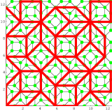
Figure 5: An approximant and its inflated version, showing the old and new tiles

where $\lambda=1+\sqrt{2}$. This irrational is fixed by the condition of eight-fold symmetry of the quasicrystal and its equivalent on the Penrose tiling is the golden mean $\tau=(\sqrt{5}+1)/2$. An important symmetry of the quasicrystal is its self-similarity under a discrete scale transformation called inflation(deflation). Fig.5 shows how to redefine the tiles or to decimate sites, so as to obtain an inflated version of the tiling. The density of sites on the infinite tiling is reduced by a factor $\lambda^{2}$ after an inflation. The rational approximants transform into each other under successive operations of inflation or deflation.

In pj , we have diagonalized the tight-binding Hamiltonian of Eq.1 for increasing system sizes, $N_{s}=239,1393,8119$, using an extended Lanczsos routine that yields all distinct energy eigenvalues.

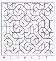
Figure 6: a)a square sample of the randomized octagonal tiling
b) a tile flip (or phason) operation

Fig.6 shows a sample obtained after one performs a certain number of operations called “phason flips” wherein one permutes the positions of a square and two rhombuses in the interior of a hexagonal shaped region. Iterating this operation at randomly chosen locations on the square approximants, one obtains a structure that has new environments that are not present in the original tiling. (Note: in the two dimensional case, contrarily to three dimensions, such randomizing leads to a reduction of the peak intensities in the structure factor henley ).

III.2 Density of states of the octagonal tiling

Typical histograms representing the density of states (DOS) for the randomized and for the perfect octagonal tiling are shown in the figures 7 and 8. (In fig.7 a delta function at $E=0$ corresponding to localized ring-like states around the eight-fold symmetric sites has been subtracted). Both graphs show a jagged dependence on the energy, with bigger fluctuations in the perfect case. The difference between the two DOS is not merely quantitative, but qualitative. The fluctuations in the randomized sample are bounded, and do not give rise to pseudogaps, where the DOS plunges to zero, as in the perfect system. When the DOS of samples of different sizes are plotted, it becomes evident that there is no smooth behavior of the DOS in the perfect case: fluctuations are strong as $N$ is varied at a fixed energy, and vice versa. This behavior is investigated in more detail below, where we consider the energy spacings for the two types of systems. A multifractal analysis pj gives a fractal dimension of the DOS equal to one, for the perfect tiling, which thus has a single band.

Figure 7: DOS of a perfect sample (from piechonthese )

Figure 8: DOS of a randomized sample (from piechonthese )

III.3 The level spacings distribution function $P(s)$ of the octagonal tiling

In analysing spacings between energy levels, one has first to classify the levels in groups according to their symmetry property. In the case of the approximants, we have one exact symmetry, namely that by reflection with respect to one of the diagonals of the square, $x=y$. There are other symmetries - the infinite tiling has a bipartite structure and so the spectrum is an even function of the energy $E$. This is broken by the approximants, but can be restored by, for example, quadrupling the unit cell so that the boundary conditions do not frustrate the wavefunctions. In addition, the approximants have an approximate rotational symmetry grimm . In the calculations mentioned below, levels were grouped according to even(odd) parity under reflection, but not separated into any further subgroups.

In most situations, it is possible to determine the unfolded spacings without any ambiguity by separating the underlying smooth energy dependence of the DOS. In the case of the randomized tiling, for example, we are able to define a locally smooth DOS and use this to renormalize spacings. The distribution obtained in pj for these renormalized spacings is shown in Fig.9, for two boundary conditions corresponding to zero and nonzero magnetic flux respectively (as explained further below). The data points are shown along with the Dyson-Wigner GOE probability distribution functions corresponding to $\beta=1$ and 2, as expected.

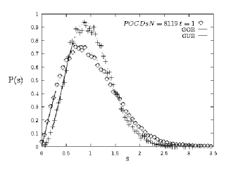
Figure 9: P(s) for the randomized octagonal tiling with and without inclusion of a magnetic flux (from piechonthese )

We found, furthermore, that the same GOE distribution is obtained when one introduces energetic (diagonal) disorder on the perfect octagonal tiling à la Anderson.

Moving on to the case of the perfect tiling, the density of states fluctuations occur on all energy scales, so that it is not obvious how to separate out a “classical” part. The same type of problem occurs at the critical point of the Anderson and the Harper models. There, it is possible to perform an averaging over all possible boundary conditions, and determine a local value of the DOS. This was used to unfold the spacings and thus obtain the critical level statistics. In the case of the quasicrystal, we first calculated the distribution of the bare spacings, i.e. without unfolding. The bare spacings turn out to follow quite well a log-normal distribution pj

$$P(s)=\frac{1}{2\pi sB}{\rm e}^{-(\ln s-\ln s_{0})^{2}/{2B}}$$ (15)

where the peak position, $\ln s_{0}$, shifts to the left as the size of the tiling is increased. This is, of course, expected as the mean level spacing decreases $\Delta\approx W/N$ where $W$ is the band width. Fig.10 shows the data for three system sizes, after the distributions were shifted so that the peaks coincide. Note that, unexpectedly, the width of the distribution, $B$, does not depend on the system size. An explanation is given in the section below where we outline the relation between the bare spacing and the unfolded spacing distributions. There are deviations from the log-normal curve: for $s$ small the distribution found is linear, and for large $s$ one finds a fit to a power law piechonthese .

Figure 10: $P(s)$ for the perfect tiling for bare spacings for $N$=239 (stars),1393 (triangles) and 8119(diamonds) (curves were shifted to that the peak positions coincide)

The log normal $P(s)$ obtained for the bare spacings corroborates a fact already noted, namely the density of states fluctuates enormously in the perfectly ordered system. Next we consider possible ways of unfolding the spacings. The standard unfolding technique, involves a smoothing of the integrated DOS as described in boh . This smoothing has to be carried out on an energy scale that is small compared to the density of states fluctuations but large compared to the average nearest neighbor spacing, a condition that is not possible to respect, strictly speaking, in a quasicrystal. In an alternative definition, we divided the spacings by the local average value of the spacing defined over M consecutive levels: $\langle s_{i}\rangle=(E_{i+M}-E_{i-M})/2M$. When M is large, then the renormalizations depend only weakly on the energy. In this case, the renormalized spacings obey a distribution close to that of the bare spacings. At the other extreme, for $M=1$, the renormalization factor fluctuates strongly from one level to the next. In this case the renormalized spacings will obey a very different probability distribution – this turns out to be the ubiquitous Wigner-Dyson distribution piechonthese . As figure 12 shows, one goes continuously from the log normal distribution to the Wigner-Dyson form simply upon changing the value of $M$ in the unfolding procedure. This was also confirmed by Zhong et al zhong using the standard unfolding procedure given in boh . A calculation of the level spacing distribution for a large but finite patch of the octagonal tiling confirmed that the same distribution is obtained in that case as well, despite the open boundary conditions grimm .

The relation between the two types of level spacing distribution is explained in terms of the heirarchical structure of the quasicrystal in the next subsection.

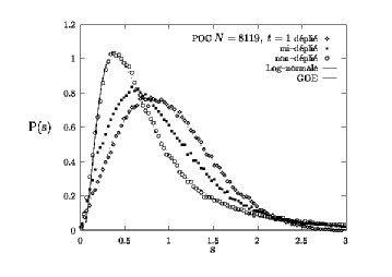
Figure 11: Statistics of levels for three cases: no level-unfolding, partial unfolding and maximal unfolding (from piechonthese )

III.4 Relation between folded and unfolded statistics

As the previous section showed, there does not appear to be a single way to define unfolded spacings for the infinite tiling, as the notion of “smoothing” is not well defined for this situation. In jagconv we have proposed a way to overcome this difficulty, which also resolves the issue of the relation between the two statistical distributions $P(s)$ and $P(\tilde{s})$. When considering level statistics of approximants, one can consider using the DOS of a smaller approximant to renormalize spacings of the next approximant in the series. Recall that approximants are related to each other by inflation/deflation transformations. In this way one can write the probability distribution of the bigger system in terms of a convolution involving the distribution function of the smaller approximant. Iterating the process, and taking the initial distribution to be of Wigner-Dyson form, one can show that after a few iterations, the distribution for the spacings approaches the log normal form. In jagconv we have analytically calculated the variance of the log normal distribution obtained in the large size limit, and we showed in particular, that it is independent of the system size, in agreement with the numerical calculations described earlier.

III.5 The effect of adding magnetic flux

The time reversal symmetry of the Hamiltonian in eq.1 can be broken by adding an external field, or, more simply, by imposing a flux via boundary conditions. This can be done by identifying two of the edges of the approximant (similarly to when one wraps a graphene sheet to form a nanotube) and considering a flux tube along the axis of the resulting cylinder. A magnetic flux $\phi$ along the axis of the cylinder will then create a total phase shift of $e^{i\pi\phi}$ on a closed loop around the flux tube. This phase shift is easily implemented by taking $\psi(x+L,y)=e^{i\pi\phi}\psi(x,y)$ $\psi(x,y+L)=\psi(x,y)$. The resulting distribution of spacings for the randomized system is GUE for sufficiently high values of $\phi$. This distribution corresponds to a stronger suppression of small spacings than in the GOE case, since now $P(s)\sim s^{2}$ for small $s$ (Eq.3). Fig. 9 shows the level statistics with and without magnetic flux, along with the theoretical GOE and GUE curves.

In the case of the perfect tiling, one cannot apply this technique to create a magnetic flux through the samples because of the exact reflection symmetry of our samples. This symmetry causes the Hamiltonian to remain in the GOE class, because it is possible to find a real symmetric representation of H even after the introduction of a flux tube through the sample ( i.e. if R is the operator for reflections $({x,y}\rightarrow{y,x})$ then H is invariant under the combined operation RT where T is the time reversal operator). GUE statistics on the octagonal tiling can still be obtained by including an external magnetic field perpendicular to the plane of the tiling in the Hamiltonian.

III.6 The spectral rigidity function of the octagonal tiling

Since level repulsion is present, wavefunctions are expected to be extended in the quasiperiodic tiling. One can expect that a wave packet initially localized in some region will spread out over time. This is now shown by an analysis of the spectral rigidity. In the randomized tiling, the spectral rigidity function crosses over from the small $E$ logarithmic law given in RMT to be $\Sigma^{2}(E)\sim\ln(E)$ to a power law behavior. It is found that

$$\Sigma^{2}(E)\propto E^{\gamma}$$ (16)

in a large range of energies, with $\gamma\approx 1.7$. The exponent for quantum diffusion is therefore determined according to eq.9 to be $\sigma\approx 0.85$. The perfect tiling shows a smaller value of the exponent, $\sigma\approx 0.8$. The result for the perfect tiling is thus in good accord with Passaro et al benza2 who found an average value 0.78 for an electron diffusing in the octagonal tiling. Our value for the random tiling is higher than the value given by those authors of 0.81. Both calculations conclude that, interestingly, diffusivity is $higher$ on the disordered tiling. Disorder thus plays a role opposite to the one it plays in a crystal, in rendering the electron more mobile.

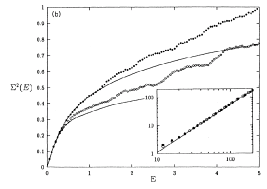
Figure 12: Spectral rigidity of the randomized tiling (solid circles: GOE; open circles: GUE). The curves correspond to RMT predictions. Inset: log-log plot of the power law region. (frompj )

III.7 Wavefunctions in the octagonal tiling

Fig.13 shows the probability distribution of an electronic state near the band edge, for one of the square approximants. One can see the typical spiky spatial dependence, with some well-defined peaks, characteristic of critical wavefunctions. Fig.14 shows results for p = P(participation ratio)/N(number of sites), plotted against the energy. Wavefunctions were investigated in detail on the Penrose tiling and are reviewed in grimm , where a similar plot is shown for the Penrose tiling. The data, in both the tilings, indicate that sites are more localized in the center of the band, compared to the edges.

Figure 13: Probability densities on sites of an approximant of the octagonal tiling for a state of energy $E\approx 3.98$

Figure 14: Plot of p =P(Participation ratio)/N for the octagonal tiling for the approximant of 1393 sites

III.8 Transport in the octagonal tiling

The results of calculations of the Thouless number in the perfect and the disordered octagonal tilings are shown in fig.15 (taken from piechonthese ). The disordered tiling has, as expected, smaller fluctuations - note the change of scale between the figures. The perfect tiling appears to have the highest value of $g_{th}$ in the center of the band but the fluctuations here are also greater. A careful study of size dependence remains to be done for this system. Early calculations on approximants of the Penrose tiling tsune2 showed that the Thouless number for that system increased towards the band edge. However, that model is dual to the vertex type model we consider here. Tsunetsugu and Ueda also calculated the conductance of strips using the multichannel Landauer formalism, and found the spiky fluctuating dependence that is a consequence of the critical wave functions and spiky density of states. They found furthermore that the wavefunctions evolve from power-law-extended to power-law-localized, as energy increased – since the tendency to open gaps increases with the energy in their model. Zijlstra has considered the octagonal tiling conductance by the same technique, but includes a potential energy term in the Hamiltonian which opens gaps in the spectrum. The results for the scaling of the conductance with size seem to indicate that despite the gaps, the wavefunctions for that system decay with power laws zijlstra .

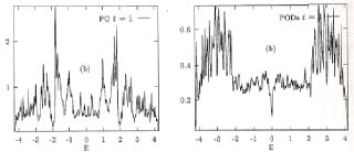
Figure 15: Thouless number for the perfect (left) and the randomized (right) tilings (from piechonthese )

IV III. A family of weakly quasiperiodic tilings

Figure 16: Rauzy tiling - a two-dimensional projection of the cubic lattice

Fig.16 shows a structure introduced by Vidal and Mosseri called a generalized Rauzy tiling vidmoss (GRT). It is obtained by projecting a cubic lattice along an irrational direction. The sample shown is an approximant, i.e., it has been constructed so as to allow periodic boundary conditions, but the infinite structure is quasiperiodic. The tight binding hamiltonian for approximants is very simple to write down contrarily to the quasicrystals discussed earlier. This is due to the fact that this lattice has a codimension of 1 (the codimension is the difference $D-d$, where $d$ is the physical dimension and $D$ the dimension of the hypercubic lattice).

For periodic approximants, the connectivity matrix is a band diagonal (Toeplitz type) matrix. The nonzero matrix elements are situated at distances of $F_{n-3},F_{n-2}$ and $F_{n-1}$ from the diagonal, where the generalized Fibonacci numbers $\{F_{n}\}$ are obtained from a three term recursion relation $F_{n}=F_{n-1}+F_{n-2}+F_{n-3}$, with the initial conditions $F_{-1}=0;F_{0}=F_{1}=1$. The ratio $F_{n}/F_{n-1}$ tends to the value $\alpha\approx 1.839...$, solution of the equation $x^{3}=x^{2}+x+1$. These matrices correspond to approximants of increasing size as $n$ is increased. For example, with $n=5$ one has a 13 site periodic problem with a site connectivity matrix $C$ given by

$$C=\left(\begin{array}[]{rrrrrrrrrrrrr}0&0&1&0&1&0&0&1&0&0&0&0&0\\ 0&0&0&1&0&1&0&0&1&0&0&0&0\\ 1&0&0&0&1&0&1&0&0&1&0&0&0\\ 0&1&0&0&0&1&0&1&0&0&1&0&0\\ 1&0&1&0&0&0&1&0&1&0&0&1&0\\ 0&1&0&1&0&0&0&1&0&1&0&0&1\\ 0&0&1&0&1&0&0&0&1&0&1&0&0\\ 1&0&0&1&0&1&0&0&0&1&0&1&0\\ 0&1&0&0&1&0&1&0&0&0&1&0&1\\ 0&0&1&0&0&1&0&1&0&0&0&1&0\\ 0&0&0&1&0&0&1&0&1&0&0&0&1\\ 0&0&0&0&1&0&0&1&0&1&0&0&0\\ 0&0&0&0&0&1&0&0&1&0&1&0&0\\ \end{array}\right)$$ (30)

It is thus not only easy to write down the Hamiltonian for big approximants for numerical calculations, but one has in this indexation of the sites a convenient basis for analytical calculations, as opposed to the octagonal and Penrose tilings.

The question now arises: are there any physical consequences of reducing the codimension ? From the point of view of geometry it seems clear that the fluctuations of the geometry will be reduced when there are fewer “degrees of freedom” in the problem. As we saw in the preceding section, a study of the eigenvalues of the tight binding Hamiltonian can yield information about the wavefunctions and the dynamics of an electron in the medium. We have already seen the use of statistical tools with which to quantify the degree of complexity of the Hamiltonian. The results obtained for the GRT in jagrauzy gave a number of insights into the similarities and differences between this quasicrystal and the ones that had been studied before, as we will now describe.

After diagonalization of the Hamiltonian, one obtains the spectrum and the DOS as shown in the figure 17. The DOS rises sharply towards the band center, recalling the van Hove singularity of the square lattice (and one sees in fig.16 that the GRT has many small patches of sites of coordination number 4). The DOS does not have the large fluctuations displayed by the octagonal tiling, instead, there appears to be an underlying smooth component to the GRT density of states. This enables us to compute the level statistics analysis using an unfolding technique similar to the one used for random systems.

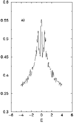
Figure 17: Density of states of the GRT

IV.0.1 Level statistics of the GRT

The distribution of spacings is not of the Wigner-Dyson type. We find instead a good fit to semi-Poisson statistics:

$$P_{sP}(s)=4s\exp^{-2s}$$ (31)

Figs.18 show the plot of the data obtained for the distribution of level spacings, along with the theoretical semi Poisson and the Poisson curves. The agreement is good over a large range of $s$, although the data falls off faster than the theoretical prediction at large $s$.

In the present case of the GRT, and the results for its $P(s)$, one can speculate that the electron motion is not integrable as in a crystal, but not chaotic as in the octagonal tiling. The GRT thus represents an intermediate case between the integrable square lattice and the nonintegrable octagonal tiling. This conclusion is in keeping with our intuition that the quasiperiodicity is, so to say, weakened due to the small codimension.

One expects, correspondingly, that the electron motion should approach the ballistic limit, with the root mean square distance travelled being linear in time $t$. This can be checked by computing the spectral rigidity function next.

Figure 18: P(s) of the GRT for three different sizes. Curves correspond to semi-Poisson and Poisson laws discussed in the text (from jagrauzy )

IV.0.2 Spectral rigidity of the GRT

The spectral rigidity corresponding to the semi Poisson case was calculated to be

$$\Sigma^{2}_{sP}(E)=\frac{1}{2}[E+\frac{1}{4}(1-\exp{-4E})]$$ (32)

which has a linear dependence at small energy, with a slope of one-half. Fig.19 shows the spectral rigidity (without unfolding) for the GRT. The behavior found agrees for small $E$, where it is linear, with a cross over to quadratic. The latter behavior at large $E$ (or short times) reflects the fact that the motion of the electron is close to ballistic, as we have already surmised and the exponent for quantum diffusion $\sigma\approx 1$.

Figure 19: Spectral rigidity of the GRT on log log scales (from jagrauzy )

An explicit calculation of the root mean square distance have been carried out by Triozon et al trio , for wave packets of varying energies. The effective exponent $\sigma$ found by these authors is about 0.9 at the center of the band, goes down to a minimum value of about 0.85 and then increases again, approaching 1 as the energy increases towards the band edge. The linear behavior of $\Sigma^{2}$ at small energies agrees with the semi Poisson formula given in Eq.32. The increased diffusivity at the band edges was found by Triozon et al trio to be accompanied by an increase of the wavefunction participation ratio (PR) as energy increases. This is reminiscent of the behavior of the IPR on the Penrose tiling described in the previous section.

One sees that the energy dependence of $\sigma$ behaves in the opposite way of what one expects in disordered systems. There, wavefunctions tend to be most delocalized at the band center, and typically get more localized as one goes out to the band edge. One can propose a handwaving explanation of this unconventional behavior in the quasicrystal. In a disordered metal, the long wavelength (low energies, close to the band center) modes are relatively less scattered by the impurities, and so these wavefunctions remain long ranged and contribute to transport. For higher energies, the wavefunctions are more sensitive to scattering and will tend to become more localized as the wave vector (and the energy) increases. In the case of the quasicrystal, for very low energies, where the wavefunction modulation is slow, the lack of translational invariance is more strongly felt compared to higher energies, where the wavefunction varies on the scale of the small crystalline patches that we alluded to earlier. This leads one to expect that the quasiperiodic fluctuations of geometry are $less$ effective in localizing the wavefunction at $high$ energies than at low energies.

V IV. Discussion and conclusions

We have presented studies of the energy level statistics in several two dimensional quasiperiodic structures and compared them with periodic as well as disordered structures.

The strong quasicrystals such as the octagonal tiling and also the Penrose tiling, are described by two different forms of the level spacing distribution. There is the distribution $P(\tilde{s})$ of the maximally unfolded spacings, where fluctuations in the density of states have been compensated down to the smallest energy scale, has the universal Dyson-Wigner form. These statistics are found irrespective of whether a geometric disorder is added or not. The tilings resemble, in this respect, other complex systems, with classically chaotic, ergodic trajectories, and the “strong” quasicrystal falls into this category. If one considers the bare unrenormalized spacings, $P(s)$ has a log normal form for both the octagonal and the Penrose winp tilings, as in some other problems involving heirarchical processes. In this case, the log normal spacing distribution reflects a heirarchical structure of the spectral density, which has huge fluctuations. The DOS for the randomized case, on the contrary, is closer to that of a typical disordered system.

We then considered a weaker quasicrystal, the generalized Rauzy tiling, obtained by projection of the simple cubic lattice. Here the spacings have a different probability distribution – the semi-Poisson law. This tiling represents an intermediate situation between the strongly chaotic and the integrable systems. The Rauzy tiling is in this respect closer to the crystal than the octagonal tiling, due to its smaller codimension.

We showed that the dynamics of the electron, as deduced from the spectral rigidity function also follows a different behavior in the strong and the weak quasicrystals: propagation with an average diffusion exponent of about 0.8 in the perfect octagonal tiling, corresponding to a superdiffusive dynamics, while having a value close to unity for the generalized Rauzy tiling, corresponding to near-ballistic propagation. Disordering the perfect octagonal tiling results in a slightly bigger value of the average exponent for anomalous diffusion.

One can ask what occurs in the limit of increasing, instead of decreasing, the codimension of the two dimensional tilings. This would result in structures having an increasing number of local environments, and increasingly stronger quasiperiodic disorder with $D$. The motion of the electrons is expected to become progressively more hampered. Destainville et al vidal2 have shown that there is no localization even in the limit of infinite $D$. As codimension is increased, the exponent for diffusion decreases, and appears to tend to the value $\sigma=0.5$ i.e. ordinary diffusion. The level spacing distribution has not been calculated, but we would expect, based on the results for the other systems discussed here, this to be Wigner-Dyson.

Finally, a word about the conductance properties of two-dimensional quasicrystals. The spectral studies described here lead us to expect that the pure hopping single component quasicrystal is close to being a metallic conductor. The quantum diffusion studies show that there are huge fluctuations as a function of the initial position of the particles, their energy, and the time elapsed - leading to some effective average behavior that is superdiffusive. Similarly, huge fluctuations occur in the Thouless number for the perfect tiling, but are attenuated in the randomized structures. The effect on the conducting properties is not well understood. This effect, as well as the detailed characteristics of this distribution remain to be investigated in detail.

- (1) R. Penrose, The Math. Intelligencer, 2 32 (1979)
- (2) D. Levine and P. J. Steinhardt in The Physics of Quasicrystals, World Scientific, Singapore 1987
- (3) D. Schechtman et al, Phys. Rev. Lett. 53 1951 (1984)
- (4) P. W. Anderson, Phys. Rev. 109 1492 (1958)
- (5) C. Sire and J. Bellissard, Europhys.Lett. 11 439 (1990); J. X. Zhong and R. Mosseri, J. Phys. I (France) 4 1513 (1994)
- (6) A. Jagannathan, Phys. Rev. Lett. 92 047202 (2004)
- (7) C. L. Henley et al, Z. Kristall. 216 1 (2001)
- (8) M. de Boissieu, Phil. Mag. 86 1115 (2006); C. L. Henley et al, Phil. Mag. 86 1123 (2006)
- (9) T. Klein et al, Phys. Rev. Lett. 66 2907 (1991)
- (10) F. S. Pierce, Q. Guo and S. J. Poon, Phys. Rev. Lett. 73 2220 (1994)
- (11) C. A. Swenson et al, Phys. Rev. B 70 094201 (2004)
- (12) J. J. Prejean et al, Phys. Rev. B 65 140203 (2002)
- (13) G. Trambly de Lassardière and D. Mayou, Phys. Rev. B 55 2890 (1997) ; E. Macia, Phys. Rev. B 66 174203 (2002); C. Janot, Phys. Rev. B 56 11338 (1998)
- (14) T. Fujiwara et al, Phys. Rev. Lett. 71 4166 (1993); S. Roche and T. Fujiwara, Phys. Rev. B 58 11338 (1998)
- (15) C. Sire in Lectures on Quasicrystals eds. F. Hippert and D. Gratias, Les Editions de Physique, Les Ulis 1994
- (16) M. Kohmoto and B. Sutherland, Phys.Rev.Lett. 56 2740 (1986)
- (17) Bill Sutherland, Phys. Rev. B 34 3904 (1986)
- (18) T. Odagaki and D. Nguyen, Phys. Rev. B 33 8879 (1986)
- (19) Vijay Kumar and G. Athithan, Phys. Rev. B 35 906 (1987)
- (20) Tetsiji Tokihiro, Takeo Fujiwara and Masao Arai, Phys. Rev. B 38 5981 (1988)
- (21) H. Tsunetsugu, T. Fujiwara, K. Ueda and T. Tokihiro, Phys. Rev. B 43 8879 (1991)
- (22) H. Tsunetsugu and K. Ueda, Phys. Rev. B 43 8892 (1991)
- (23) Vincenzo G. Benza and Clément Sire, Phys. Rev. B 44 10343 (1991)
- (24) B. Passaro, C. Sire and V. G. Benza, Phys. Rev. B 46 13751 (1992)
- (25) A. Jagannathan, J. Phys. (France) I4 133 (1994)
- (26) F. Piéchon and A. Jagannathan, Phys. Rev. B 51 179 (1995)
- (27) J. X. Zhong et al, Phys. Rev. Lett. 80 3996 (1998)
- (28) E. S. Zijlstra and T. Janssen, Phys. Rev. B 61 3377 (2000)
- (29) E. S. Zijlstra, Phys. Rev. B 66 214202 (2002)
- (30) B. Kramer and A. MacKinnon, Rep. Prog. Phys. 56 1469 (1993); T. Ohtsuki et al, Ann. der Physik, 8 655 (1999)
- (31) see http://www.geom.umn.edu/apps/quasitiler/about.html
- (32) O. Bohigas in Mathematical and Computational Methods in Nuclear Physics eds. J.S. Dehesa and J.M.G. Gomez and A. Polls, 209, Springer (Berlin) 1984
- (33) M.L. Mehta, Random Matrices, Academic Press, Boston (1991)
- (34) B. I. Shklovskii et al, Phys. Rev. B 47 11487 (1993)
- (35) J. T. Chalker et al, JETP Lett. 64 386 (1996);J. T. Chalker et al, Phys.Rev.Lett. 77 554 (1996); J. Math. Phys. 37 5061 (1996)
- (36) V.E. Kravtsov et al, Phys.Rev.Lett. 72 888 (1994)
- (37) S. N. Evangelou, Phys. Rev. B 49 16805 (1994)
- (38) D. Braun and G. Montambaux, Phys. Rev. B 52 13903 (1995)
- (39) M. Batsch, L. Schweitzer, I.Kh. Zharekeshev and B.Kramer, Phys. Rev.Lett. 77 1552 (1996)
- (40) X. Waintal et al, Europ. Phys. J. B 7 451 (1999)
- (41) S. N. Evangelou and J.-L. Pichard, arXiv:cond-mat/9902321 (1999)
- (42) E.B. Bogomolny and U. Gerland and C. Schmit, Phys. Rev. E 59 R1315 (1999)
- (43) N. Argaman and Y. Imry and U. Smilansky, Phys. Rev. B 47 4440 (1993)
- (44) Eric Akkermans and Gilles Montambaux, Physique mésoscopique des électrons et des photons, EDP Sciences/CNRS Editions, Les Ulis (2004)
- (45) U. Grimm and M. Schreiber in Quasicrystals - Structure and Physical Properties, ed. H.-R. Trebin (Wiley-VCH, Weinheim, 2003)
- (46) S. N. Evangelou, J. Phys. A 23 L317 (1990)
- (47) D. J. Thouless, Phys. Rev. Lett. 39 1167 (1975)
- (48) C. Basu et al, Phys. Rev. B 57 14174 (1998)
- (49) C. Canali et al, Phys. Rev. B 54 1431 (1996); M. Titov et al, J. Phys; A 30 L339 (1997)
- (50) M. Duneau, Remy Mosseri and Christophe Oguey, J. Phys. A 22 4549 (1989)
- (51) J. E. S. Socolar, Phys. Rev. B 39 10519 (1989)
- (52) M. Duneau, Lecture Notes, Marakesh Winter School (2002)
- (53) M. Baake and D. Joseph, Phys. Rev. B 42 8091 (1990)
- (54) F. Piéchon, Ph.D. thesis, Université Paris-Sud (1995)
- (55) A. Jagannathan, Phys. Rev. B 61 R834 (2000)
- (56) J. Vidal and R. Mosseri, J. Phys. A 34 3927 (2001)
- (57) A. Jagannathan, Phys. Rev. B 64 140201 (2001)
- (58) Francois Triozon, Julien Vidal, Remy Mosseri and Didier Mayou, Phys. Rev. B 65 220202 (2002)
- (59) Julien Vidal, Nicolas Destainville and Remy Mosseri, Phys. Rev. B 68 172202 (2003)
- (60) A. Jagannathan and A. Szallas, unpublished