Stresses in smooth flows of dense granular media

Abstract

The form of the stress tensor is investigated in smooth, dense granular flows which are generated in split-bottom shear geometries. We find that, within a fluctuation fluidized spatial region, the form of the stress tensor is directly dictated by the flow field: The stress and strain-rate tensors are co-linear. The effective friction, defined as the ratio between shear and normal stresses acting on a shearing plane, is found not to be constant but to vary throughout the flowing zone. This variation can not be explained by inertial effects, but appears to be set by the local geometry of the flow field. This is in agreement with a recent prediction, but in contrast with most models for slow grain flows, and points to there being a subtle mechanism that selects the flow profiles.

1 Introduction

Granular media are amorphous and athermal materials which can jam into stationary states, but which can also yield and flow under sufficiently strong external forcing [1, 2]. Slowly flowing granulates, for which momentum transfer by enduring contacts dominates over collisional transfer, are characterized by a yielding criterion and rate independence. The former expresses that granulates only start to flow when the applied shear stresses exceed a critical yielding threshold [1, 2, 3], while the latter signifies that a change in the driving rate leaves both the spatial structure of the flow and the stresses essentially unaltered [4, 5, 6, 7, 8].

Solid friction exhibits a similar combination of yielding and rate-independence: According to the Coulomb friction law, a block of material resting on an inclined plane starts to slide when its ratio of shear to normal forces exceeds the static friction coefficient. And, once the block slides, the same ratio is given by a lower dynamical friction coefficient, which is essentially rate independent.

There is no unique manner in which these friction laws can be translated into a continuum theory, and there exists a plethora of approaches describing slow granular flows [3, 8, 9, 10, 11, 12, 13, 14]. To test these theories, one would like to determine the stresses and strain rates within the material. However, experiments can not easily access the flow in the bulk of the material, nor probe the stress tensor in sufficient detail. In addition, slow grain flows often exhibit sharp gradients, thus casting doubt on the validity of continuum theories [3, 4, 5, 6, 9]. Finally, granular flows are notoriously sensitive to subtle microscopic features [5], which often translates into a substantial number of tunable parameters in the models [10]. As far as we are aware, no direct comparison between the full stress and strain rate tensor has been undertaken for slow granular flows.

In this Letter, we numerically study grain flows in split-bottom geometries as shown in fig. 1. Recently, these flows were shown to exhibit robust and continuum-like flow profiles that are numerically tractable and are governed by a number of universal, i.e. grain-independent, scaling relations, making them eminently suitable for our purpose. We relate the stress tensor to the strain-rate tensor in these flows, thus providing a benchmark for the testing and development of theoretical models for smooth and dense grain flows. Experiments and numerics so far have focussed on the flow in a cylindrical geometry (fig. 1c), where a wide shear zone is generated by rotating a centre bottom disc with respect to the cylindrical container [7, 14, 15]. We present some data for this cylindrical case, but focus on the linear version of this geometry (fig. 1a), where we find a wide shear zone to emanate from the relative motion of two bottom plates along their “fault line”. In this system, the physics behind the stresses is easier to disentangle because the stream lines are not curved.

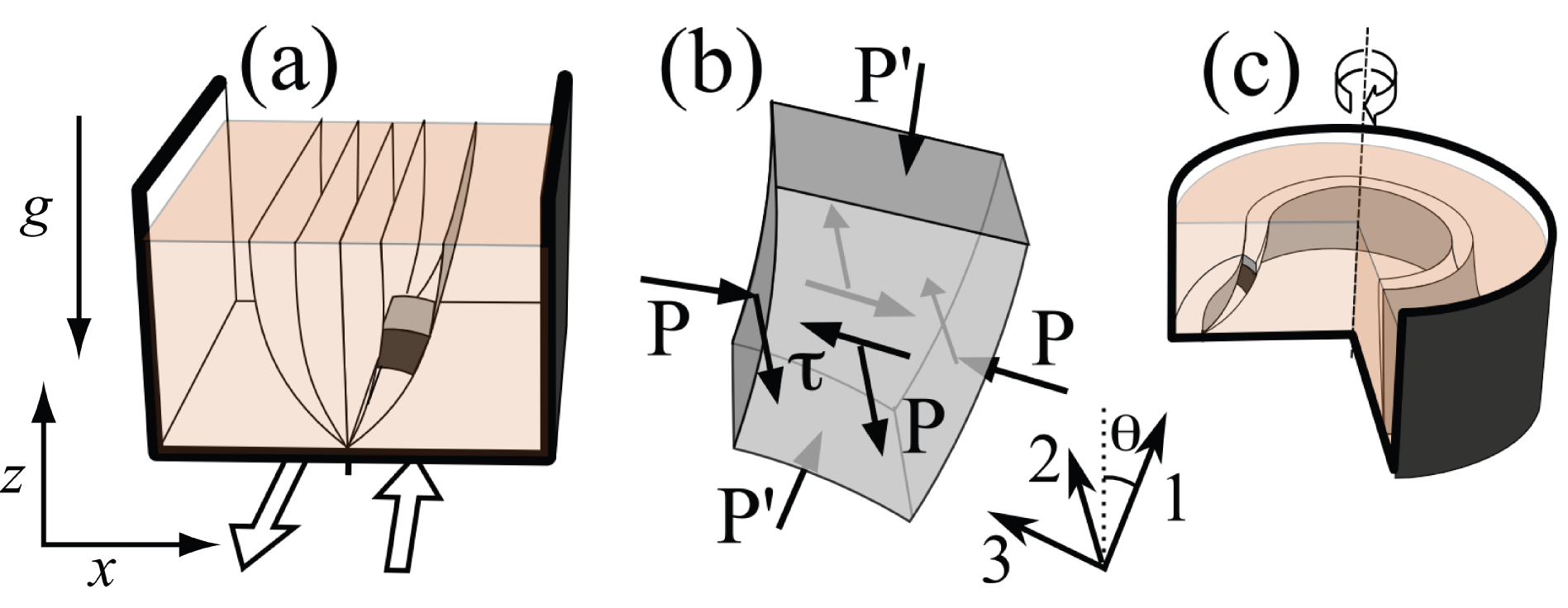
Figure 1: (a) Linear shear geometry where a split along the middle of the system generates a wide shear zone in a layer of grains. The curves indicate sheets of constant velocity. (b) Cuboid element of material showing the definition of the angle $\theta$, the stresses in the SFS framework, and the labelling of the axis — the grey objects in a) and c) are examples of such elements. (c) Cylindrical split-bottom geometry, where the grains are driven by the rotation of a bottom disc. The two surfaces of rotation indicate sheets of constant angular velocity. Note that in the limit $R_{s}\!\to\!\infty$ one obtains the linear geometry (a).

Our main finding is that, throughout the flowing zone, the stress and strain tensor are co-linear, meaning that their eigen-directions, or equivalently, their principle directions, coincide. Moreover, we find that the ratios of the non-zero stress components, such as the effective friction coefficient, which is the ratio between shear and normal stresses acting on a shearing plane, are not constants but vary throughout the flowing zone. This variation is crucial to understand the finite width of the shear zones, and is not due to the variation in the magnitude of the local strain rate. Both of these findings are in accord with the main features of theory developed in [8], and constitute an important step forward in establishing a general framework for the modelling of grains flows.

2 SFS framework

We formulate our results in the context of the theoretical framework recently developed by Depken et al. [8]. The central assumption of this so-called SFS theory is that, once the material is flowing, strong fluctuations in the contact forces enable otherwise jammed states to relax within a spatial region which we refer to as the fluctuation fluidized region. In this region there can not be a shear stress without a corresponding shear flow. This assumption can be interpreted as stating that the yielding threshold, which determines the onset of flow, is no longer relevant once part of the material flows, since this induces strong non-local fluctuations in the contact forces. Further one observes that the flows can be locally (and in the present cases also globally) seen as comprised of material sheets, with no internal average strain rate, sliding past each other (see fig. 1).

Combining these two ingredients, it follows that both the shear strains and shear stresses in these material sheets are zero, and we refer to them as a Shear Free Sheet (SFS). It also follows that the stress and strain-rate tensors are co-linear. The major and minor principle directions of the strain-rate tensor are at an angle of 45^∘ with respect to the SFSs, and in the more intuitive basis specified by these sheets (see fig. 1b) the stress tensor takes the form:

$$\sigma_{{\rm SFS}}=\left(\begin{array}[]{ccc}P^{\prime}&0&0\\ 0&P&\tau\\ 0&\tau&P\end{array}\right)~{}.$$ (1)

To test this prediction, we check whether the numerically obtained stresses are co-linear with the strain rate tensor and thus are of the form (1). Moreover, when no further assumptions are made, the three components $P$, $P^{\prime}$, and $\tau$ will be different, and in general vary throughout the sample. In fact, if the stress is of this form, a simple stress balance argument shows that $\mu_{\rm eff}:=\tau/P$ has to vary throughout the shear zones [8]: A constant $\mu_{\rm eff}$ would correspond to a shear zone of zero width, clearly inconsistent with the available data [7, 15].

To put these predictions in perspective, let us briefly consider the case of faster flows, where collisions play a role. The arguments for the form of the stress tensor can be extended to apply also for such systems, and Pouliquen and co-workers [13] have suggested that the stress is of the form eq. (1). However, they introduce the following restriction: $P^{\prime}\!=\!P$ and $\tau=\mu_{\rm eff}(I)P$, where the effective friction is a material dependent function of the so-called inertial number $I=\dot{\gamma}d/\sqrt{P/\rho}$ [16], and $d$ and $\rho$ are the particles diameter and density, respectively [12, 13]. For the slow flows under consideration here, we should consider the limit $I\to 0$. If we only consider $\mu_{\rm eff}$ to depend on $I$, $\mu_{\rm eff}$ becomes a material constant, which is, as we explained above, incompatible with the finite width of the shear zones [8, 14, 17]. Our study will thus illuminate how subtle details of the form of the stress tensor have significant consequences for the grain flow.

3 Method

The simulations are carried out with a discrete element method (DEM) for $80\!-\!100$k mono-disperse Hertzian spheres satisfying the Coulomb friction laws. The relevant parameters describing the material properties of the spheres are the normal stiffness $k_{n}=2\times 10^{5}mg/d$, the tangential stiffness $k_{t}=2/7k_{n}$, the normal and the tangential viscous damping coefficients $\gamma_{n}=50\sqrt{g/d}$ , $\gamma_{t}=0$, and the microscopic coefficient of friction $\mu_{m}=0.5$. Here $d$ and $m$ are the diameter and the mass of spheres, and $g$ is the gravitational acceleration. The characteristic timescale $t_{0}$ is given by $\sqrt{d/g}$ (e.g., $t_{0}=0.0101sec$ if $d=1mm$). We have studied a range of driving rates varying from from $\pm 0.05$ to $\pm 0.005~{}d/t_{0}$ and $0.015$ to $0.005~{}rad/t_{0}$ for the linear and circular geometries, respectively. Stresses and velocities are averaged over the symmetry direction (along split) and are resolved with a resolution of $0.9d$ in the cross section. The stress tensor within this volume is the sum of contact and collisional stresses [18], where the latter is three orders of magnitude smaller than the former. The linear setup has dimensions $20d$ in the shearing direction (periodic boundary conditions), a width of $80d$, and a height of $50d$. The details of the specific implementation can be found elsewhere [18].

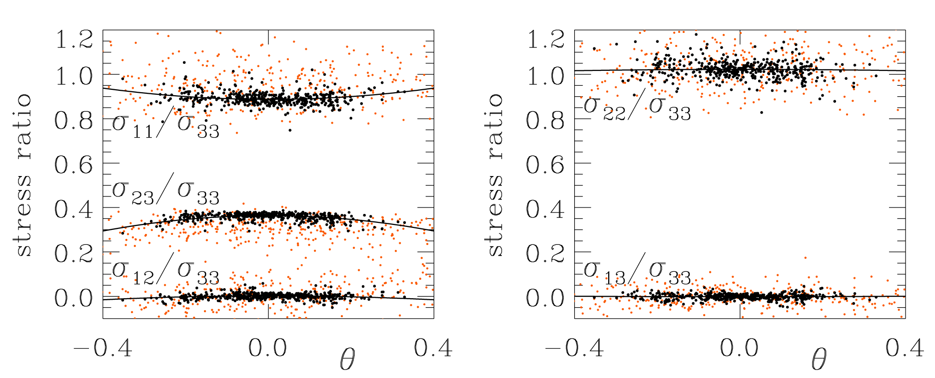
Figure 2: Stress ratios $\sigma_{ij}/\sigma_{33}$ in the linear geometry. The data was taken for a run where the velocity difference across the sliding bottom plates was 0.05 $d/t_{0}$, and was averaged over the time interval ranging from 7150 $t_{0}$ to 9150 $t_{0}$ — similar results where obtained for a velocity difference that was ten times smaller. We plot the data as a function of $\theta$, the angle between the ”1” direction of the SFS basis (see fig. 1) and the vertical. Black (red) dots refer to points inside (outside) the fluctuation fluidized zone (see text), and the curves are quadratic fits to the data in this zone. The stress tensor follows eq. (1): The ratios $\sigma_{12}/\sigma_{33}$, $\sigma_{13}/\sigma_{33}$ and $\sigma_{22}/\sigma_{33}$ are very close to zero, zero and one, while the ratios $\sigma_{11}/\sigma_{33}=P^{\prime}/P$ and $\sigma_{23}/\sigma_{33}=\mu_{\rm eff}$ vary with $\theta$ and do not attain any special value.

4 The form of the stress tensor

We first study the relation between stresses and strain rates in the linear geometry. Through a cross section of the flow we record the time-averaged stress and velocity fields, and from the latter we extract the orientation of the SFS basis. In the region far away from the shear zone, these fields fluctuate strongly, and we limit the analysis to a “fluctuation fluidized zone”. For this particular data set we take the boundary of the fluctuation fluidized zone to be defined by where the inertial number $I$ attains the value $I_{\rm cut}=4\times 10^{-5}$ — why this is reasonable is detailed below.

Within this zone, we express the stresses in the SFS basis, and compare our numerically obtained stresses to the SFS form (1). We find that, due to gravity, all stress components grow roughly proportional with depth. Since the SFS theory makes no prediction on the absolute values of the various stress components, we focus on the stress ratios $\sigma_{ij}/\sigma_{33}$ (note that $\sigma_{23}/\sigma_{33}$ directly yields the effective friction coefficient, $\mu_{\rm eff}$).

In fig. 2 we plot the stress ratios as a function of the angle $\theta$, which parameterizes the orientation of the SFS basis with respect to gravity (see fig. 1b). Even though the stress ratios could vary arbitrarily with position throughout the cross section, we find that their main variation is with $\theta$ — the relevance of this angle will be discussed below. Figure 2 illustrates that in the fluctuation fluidized zone the stress tensor takes the SFS form (1). First, all stress ratios within this region appear to collapse on single curves when plotted as function of $\theta$, while data outside the region is scattered more strongly. Second, the values for the ratio’s $\sigma_{12}/\sigma_{33}$ and $\sigma_{13}/\sigma_{33}$ scatter around zero. Third, the ratio $\sigma_{22}/\sigma_{33}$ is close to one and does not vary with $\theta$. Together these points show the validity of the SFS picture within the fluctuation fluidized region (see below for a more precise definition). Finally, the stress ratios $\sigma_{11}/\sigma_{33}=P^{\prime}/P$ and $\sigma_{23}/\sigma_{33}=\tau/P$ are not constant and do not attain any special values. The data does not suggest that it is possible to simplify the form of the stress tensor (1) any further.

5 Angle dependence of stress

The variation of the effective friction $\mu_{\rm eff}$ with angle $\theta$ takes on a special significance in the linear geometry. In [8] it was shown that, given a stress tensor of the SFS form, force balance dictates that $\mu_{\rm eff}$ attains its maximum in the middle of the shear zone, where $\theta\!=\!0$. It was further shown that the curvature of $\mu_{\rm eff}(\theta)$ could be directly related to the scaling of the width of the shear zone with vertical position in the sample; $W\sim z^{\alpha}$, $\alpha=1/(1+\partial_{\theta\theta}\mu_{\rm eff}|_{\theta=0})$. For constant $\mu_{\rm eff}$, $\alpha\!=\!1$ and the shear zones become of zero width [8, 14, 17].

As fig. 2a shows, $\mu_{\rm eff}$ varies by roughly 10% throughout the fluctuation fluidized region and indeed attains a maximum in the middle. A quadratic fit to $\mu_{\rm eff}$ yields that $\partial_{\theta\theta}\mu_{\rm eff}|_{\theta=0}\approx 2.5[5]$, which suggests the scaling exponent $\alpha=0.35[5]$. From the numerical data presented here, and from the data in [7] and [15], the value of this width exponent can be estimated to be somewhere in the range $0.25-0.4$, consistent with our estimate [19]. We interpret this coincidence as a strong check on the validity of the SFS form — the variation of $\mu_{\rm eff}$ is clearly a subtle effect, and one could imagine that small and systematic deviations of the stresses from the SFS form could destroy the relation between $\alpha$ and $\partial_{\theta\theta}\mu_{\rm eff}|_{\theta=0}$.

6 Spatial variation of the stress

In fig. 3 we plot the variations of the stress ratios $\sigma_{ij}/\sigma_{33}$ throughout a cross section of the linear cell, including data from outside the fluctuation fluidized zone. We will now provide support for our assertion that the dominant variations of the stress ratios are with $\theta$. We first checked that the correlation between $\mu_{\rm eff}$ and dimensionless quantities, such as the density and the curvatures of the SFS basis, are unconvincing. Other potential candidates are $\theta$, $\dot{\gamma}$, and $I$, and these are also shown fig. 3. Figure 3 shows that the spatial variation of $\mu_{\rm eff}$ is closer to $\theta$ than it is to $\dot{\gamma}$ or $I$.

Moreover, if the variation of $\mu_{\rm eff}$ was dominated by the variation of $I$ or $\dot{\gamma}$, one would expect the width of the shear zones to strongly depend on the shear rate — in stark contrast to both experimental [7, 15] and numerical data [15]. In fact, in runs done for a driving rate which is a factor 10 smaller than shown here, the stresses, flow profiles and $\mu_{\rm eff}(\theta)$ are indistinguishable from those reported here — the system is truly rate independent. Finally, for the small inertial numbers here, $d\mu_{\rm eff}/dI\sim{\cal O}(1)$ (based on the data presented in [12]), while variations in $I$ over the shear zone are ${\cal O}(10^{-3})$ — far too small to explain the 10% variation in $\mu_{\rm eff}$.

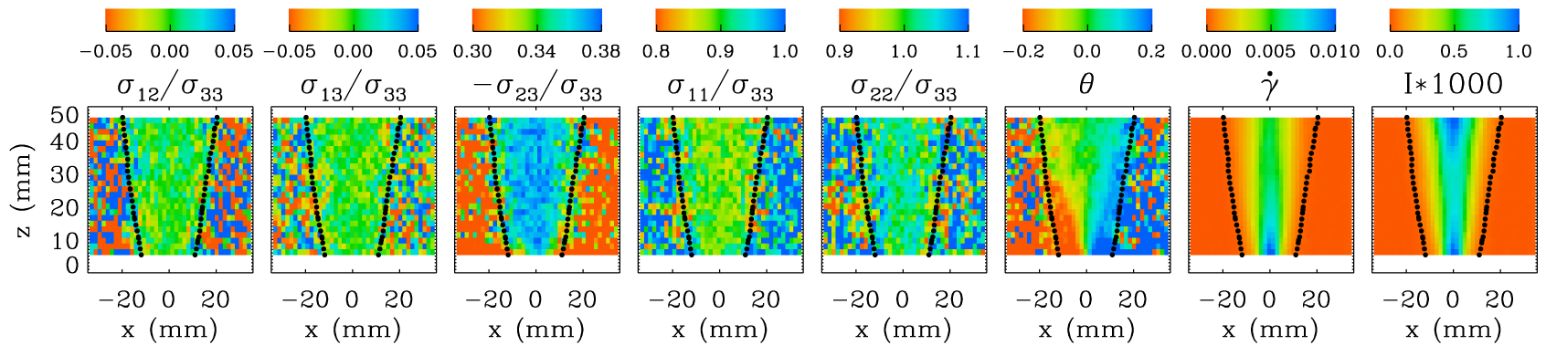
Figure 3: Components of the stress tensor in the SFS basis for the linear shearing geometry, compared to the angle $\theta$, local strain rate $\dot{\gamma}$ and inertial number $I$. This data is based on the same run as shown in fig. 2. A qualitative change of behavior of the stress fields is clearly visible around the dashed lines, which indicates the boundary of what is taken as the fluctuation fluidized zone, $I=I_{\rm cut}=4\times 10^{-5}$ (see text).

7 The fluctuation fluidized region

Central to the SFS picture is that shear flows induce force fluctuations that spread through and fluidize the material, thus eliminating the yield stress. How far do these fluidized zones spread? As can be seen in Figs. 2 and 3, there is a clear region within which the stresses satisfy the SFS form of eq. (1), while outside this region the stresses become noisy. We initially expected the total local strain experienced since the start of the numerical experiment, $\dot{\gamma}t$, to distinguish regions where fluctuations have allowed the stresses to relax to the SFS form. But, when attempting to maximize the spatial region of co-linearity, we found that the inertial number, $I$, leads to a better estimate of the fluctuation fluidized region: For the same required accuracy in co-linearity, a larger region is selected [16]. In Figs. 2 and  3, the region is defined as $I>I_{\rm cut}=4\times 10^{-5}$. It should be noted that this cut-off does not define a region of visible shear (as seen from the $\dot{\gamma}$ plot in fig. 3), but rather a region within which the microscopic fluctuations, created mainly in the region of relatively large strain rates, remove any static shear resistance.

Can we understand the numerical value of $I_{\rm cut}$? The total strain experienced after $t=8000~{}t_{0}$ (taken in the middle of the total time-interval over which the stresses are averaged) equals $8000~{}t_{0}~{}\dot{\gamma}=8000~{}\sqrt{d/g}~{}\dot{\gamma}$. At the edge of the fluctuation fluidized zone at a certain height $z$, the local strain rate equals $I_{\rm cut}/d~{}\sqrt{P/\rho}=I_{\rm cut}\sqrt{g(h-z)}/d$; hence the total strain experienced at this edge equals $8000~{}I_{\rm cut}~{}\sqrt{(h-z)/d}=0.32~{}\sqrt{(h-z)/d}$. Near the bottom the total strain thus approximates five, while near the surface it becomes of order 0.3. Even though the fluctuation fluidized region is not directly given by $\gamma$, these numbers nevertheless set a reasonable scale for the amount of strain the material needs to experience before it is fluidized, in particular if one realizes that due to the pressure gradient, the strain near the bottom couples more strongly to the fluctuations of the forces near the surface than vice versa. It should also be noted that we do not expect the numerical value of $I_{\rm cut}$ to be universal — in particular, for longer runs we expect the fluctuation fluidized region to spread slowly, with $I_{\rm cut}\sim 1/t$.

8 Results in cylindrical geometry

In fig. 4 we show simulation results for a cylindrical geometry with $H/R_{s}=0.675$ — similar results are reached for a number of other filling heights not shown here [20]. Figure 4 shows that also for the curved geometry, the stresses are in the SFS form: The values for the ratio’s $\sigma_{12}/\sigma_{33}$, $\sigma_{13}/\sigma_{33}$ and $\sigma_{22}/\sigma_{33}$ scatter around zero, zero, and one respectively, with the ratio’s $\sigma_{11}/\sigma_{33}=P^{\prime}/P$ and $\sigma_{23}/\sigma_{33}=\tau/P$ varying throughout the fluctuation fluidized zone.

Note that due to the more complex curved geometry, we have no a-priori theoretical reason for expecting the stress ratios to vary with $\theta$ alone. Moreover, there is no reason that $\mu_{\rm eff}$ should be maximal in the middle, nor is it known how $\mu_{\rm eff}(\theta)$ would be related to the width of the shear zones — if at all.

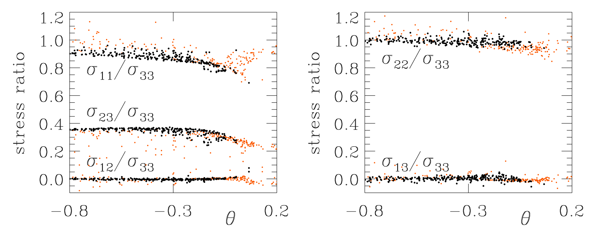
Figure 4: Stress ratios $\sigma_{ij}/\sigma_{33}$ as a function of $\theta$, for a circular geometry. The driving rate $\Omega$ was equal to 0.015 rad/$t_{0}$, and averages where taken for time ranging from 8000 $t_{0}$ to $10^{4}$ $t_{0}$, corresponding to the interval from approximately 19 to 24 turns. We have checked that similar results where obtained for a run with $\Omega$ equal to 0.005 rad/$t_{0}$. As before, black (red) dots referring to points inside (outside) the fluctuation fluidized zone. For details, see text.

9 Conclusion and Outlook

Based on the single, straightforward and minimal assumption that fluctuations on the grain scale forbid the occurrence of shear stresses without an associated shear flow, it was in [8] predicted that the stress tensor in slow grain flows should take the form (1), with the stress ratios varying throughout the sample. The data presented here fully confirms this prediction: (i) In the flowing zones, the stresses indeed take the form (1). The three different components $P^{\prime}$, $P$ and $\tau$ are sufficiently different that no further simplifications are consistent with the data. (ii) The ratio $P^{\prime}/P$ and the effective friction $\mu_{\rm eff}=\tau/P$ are not constant. (iii) The variation of $\mu_{\rm eff}$ can be directly related to the width of the shear zones. (iv) For the cylindrical geometry, the stress tensor also satisfies the SFS criteria, with $P^{\prime}/P$ and $\mu_{\rm eff}=\tau/P$ varying over the shear zone, but due to the more complex geometry we can not relate this variation directly to the width of the shear zones.

The SFS approach thus provides a powerful framework for unraveling the relations between flow and stresses in granular media in general, and the crucial but subtle spatial variation of the effective friction $\mu_{\rm eff}$ and the unexpected variation of $P^{\prime}/P$ in particular.

The range of validity of the SFS approach is not yet clearly mapped out, and additional studies to answer the following key questions are called for. (i) How does the stress tensor evolve when the flow rate is increased? The stress tensor in the Pouliquen approach for fast flows is similar to ours, but with the restrictions that $P^{\prime}\!=\!P$ and that $\mu_{\rm eff}(I)$ is a function of the local strain rate only [13]. Here $\mu_{\rm eff}$ apparently depends on geometry, and the crossover from geometry ($\theta$) to inertial number ($I$) dependence needs to be explored. (ii) We have seen here that $P$ and $P^{\prime}$ are systematically different, as was also seen in simulations of chute flows [18], and moreover, that $P^{\prime}/P$ is not a constant. Though we do not understand the cause, nor the precise relevance, of this, it can not be a priori ignored given the crucial role played by such variation of $\mu_{\rm eff}$ in the formation of the wide shear zones in the linear geometry. (iii) What distinguishes the zone where the stresses are in the SFS form from the region where they are not? Underlying the SFS picture is the assumption that the fluctuations are sufficiently strong and fast, and one imagines that far away from the shear zones this no longer holds true, thus leading to a breakdown of co-linearity. Preliminary data suggest, however, that the fluctuation fluidized region, most of which is established after a short transient, very slowly expands as a function of time [20]. Possibly, after sufficiently long time, all the material has experienced flow and the stress tensor takes the SFS form everywhere, but this may be hard to verify numerically. Similar questions on the validity of the SFS framework can also be asked when the driving rate is made excessively slow. Ultimately, these questions are related to the puzzling nature of the transition between the static and flowing state of granular media [18, 21]. (iv) Is the variation of the effective friction the cause or effect of the smoothness of our shear profiles? We suggest that the spreading of contact force fluctuations, from the rapidly shearing center to the tails of the shear zones, may elucidate the microscopic mechanism by which the width of the shear zones are selected. In this picture, the spread of fluctuations would also drive the subtle variations of the coarse grained and time averaged stresses, which thus serve to signal an underlying, but unknown, fluctuation driven mechanism [22].

- [1] A.J. Liu and S.R. Nagel, Nature 396, 21 (1998).
- [2] H. M. Jaeger, S. R. Nagel and R. P. Behringer, Rev. Mod. Phys. 68, 1259 (1996).
- [3] R. M. Nedderman, Statics and Kinematics of Granular Materials, Cambridge University Press (Cambridge), 1992
- [4] C.T. Veje, D.W. Howell and R.P. Behringer, Phys. Rev. E 59, 739 (1999).
- [5] D. M. Mueth, G. F. Debregeas, G. S. Karczmar et al., Nature 406 385 (2000).
- [6] F. Da Cruz, F. Chevoir, D. Bonn et al., Phys. Rev E 66 051305 (2002).
- [7] D. Fenistein and M. van Hecke, Nature 425, 256 (2003); D. Fenistein, J. W. van de Meent and M. van Hecke, Phys. Rev. Lett. 92, 094301, (2004); ibid. Phys. Rev. Lett. 96 118001 (2006).
- [8] M. Depken, W. van Saarloos, and M. van Hecke, Phys. Rev. E 73, 031302 (2006).
- [9] L. Bocquet, J. Errami and T. C. Lubensky, Phys. Rev. Lett. 89, 184301 (2002).
- [10] I. S. Aranson, L. S. Tsimring, Phys. Rev. E 64, 020301 (2001)
- [11] C. H. Rycroft, M. Z. Bazant, G. S. Grest and J. W. Landry, Phys. Rev. E 73 051306 (2006).
- [12] GDR MiDi, Eur. Phys. J. E 14, 367, (2004).
- [13] P. Jop, Y. Forterre, O. Pouliquen, Nature 441, 727 (2006)
- [14] T. Unger, J. Kertész and D.E. Wolf, Phys. Rev. Lett. 94, 178001 (2005).
- [15] X. Cheng, J. B. Lechman, A. Fernandez-Barbero et al. Phys. Rev. Lett. 96, 038001 (2006).
- [16] The inertial number can be seen as the ratio of the characteristic timescale for a grain to relax back from a local dilation event () to the strainrate ().
- [17] P. Jop, private communications.
- [18] L. E. Silbert, D. Ertas, G. S. Grest, T. C. Halsey, D. Levine, and S. J. Plimpton, Phys Rev E 64 051302 (2001).
- [19] The error bar on is based on its variation with , when this cutoff ranges from to .
- [20] J. B. Lechman, M. Depken, M. van Hecke, W. van Saarloos and G. S. Grest, in preparation.
- [21] E. I. Corwin, H. M. Jaeger and S. R. Nagel, Nature 435, 1075 (2005).
- [22] J. Török, T. Unger, J. Kertesz and D. E. Wolf, Phys. Rev. E 75, 011305 (2007)