Phase Separation of Charge-Stabilized Colloids:
A Gibbs Ensemble Monte Carlo Simulation Study

Abstract

Fluid phase behavior of charge-stabilized colloidal suspensions is explored by applying a new variant of the Gibbs ensemble Monte Carlo simulation method to a coarse-grained one-component model with implicit microions and solvent. The simulations take as input linear-response approximations for effective electrostatic interactions – hard-sphere-Yukawa pair potential and one-body volume energy. The conventional Gibbs ensemble trial moves are supplemented by exchange of (implicit) salt between coexisting phases, with acceptance probabilities influenced by the state dependence of the effective interactions. Compared with large-scale simulations of the primitive model, with explicit microions, our computationally practical simulations of the one-component model closely match the pressures and pair distribution functions at moderate electrostatic couplings. For macroion valences and couplings within the linear-response regime, deionized aqueous suspensions with monovalent microions exhibit separation into macroion-rich and macroion-poor fluid phases below a critical salt concentration. The resulting pressures and phase diagrams are in excellent agreement with predictions of a variational free energy theory based on the same model.

I Introduction

Charge-stabilized colloidal suspensions pusey containing monovalent microions reportedly can display unusual thermodynamic behavior when strongly deionized. Puzzling experimental observations include liquid-vapor coexistence tata92 , stable voids ise94 ; ise96 ; tata97 ; ise99 , contracted crystal lattices matsuoka ; ise99 ; groehn00 , and metastable crystallites grier97 . Such phenomena reveal an extraordinary cohesion between like-charged macroions that appears inconsistent with the purely repulsive electrostatic pair interactions predicted by the classic theory of Derjaguin, Landau, Verwey, and Overbeek (DLVO) DL ; VO . Failure of the DLVO theory to account for anomalous phase behavior of deionized suspensions has prompted many theoretical and simulation studies.

Predictions of a spinodal instability in deionized charged colloids follow from classical density-functional vRH97 ; vRDH99 ; vRE99 ; zoetekouw_pre06 , extended Debye-Hückel warren00 ; chan85 ; chan01 , and linear-response silbert91 ; denton99 ; denton00 ; denton04 ; denton06 theories of a coarse-grained one-component model. The predicted phase separation is driven by the state dependence of the effective electrostatic interactions, including a one-body volume energy hansen-lowen00 ; belloni00 ; levin02 . Such predictions have been challenged on grounds that underlying linearization approximations may fail to describe nonlinear microion screening vongrunberg01 ; deserno02 ; tamashiro03 and neglect strong counterion association that may renormalize the effective macroion charge levin98 ; levin01 ; levin03 ; levin04 ; zoetekouw_prl06 . The debate is somewhat complicated, however, by the proximity of the unstable parameter regime to the threshold for significant nonlinearity and charge renormalization.

Some simulations of the primitive model linse00 ; hynninen05 , with explicit microions interacting via long-ranged Coulomb potentials, exhibit clustering of macroions at strong electrostatic couplings. Such computationally intensive simulations become increasingly demanding, however, upon approaching the size and charge asymmetries required to directly test predictions, even when sophisticated cluster moves are included luijten04 . Therefore, reconciling theories, simulations, and experiments to clarify the phase behavior of deionized charged colloids calls for novel simulation methods tailored to mesoscale models.

The main purpose of the present work is to propose a new variant of the Gibbs ensemble Monte Carlo method suited to modeling density-dependent effective electrostatic interactions. As a demonstration, we apply the method to deionized charged colloids to test predictions of phase instability. After first defining the model system and one-component mapping in Sec. II, we briefly summarize the linear-response theory of effective interactions and a variational free energy theory in Sec. III. The Monte Carlo algorithm is next outlined in Sec. IV. Simulation results are presented in Sec. V, with diagnostic details deferred to the Appendix. Comparisons with theory and primitive model simulations confirm previous predictions and illustrate computational advantages and limitations of the one-component model. Finally, Sec. VI summarizes our conclusions.

II Model

II.1 Primitive Model

As underlying microscopic model, we adopt the primitive model of charged colloids HM : macroions and microions dispersed in a continuum solvent of dielectric constant $\epsilon$ in a closed volume $V$. The macroions are modeled as charged hard spheres, monodisperse in radius $a$ and effective valence $Z$ (charge $-Ze$), and the microions (counterions and salt ions) as point charges of valence $z$. Here we assume monovalent microions ($z=1$) dispersed in water at temperature $T=293$ K, corresponding to a Bjerrum length $\lambda_{B}\equiv e^{2}/(\epsilon k_{B}T)=0.72$ nm. Assuming $N_{m}$ macroions and $N_{s}$ pairs of dissociated salt ions, we have $N_{+}=(Z/z)N_{m}+N_{s}$ positive and $N_{-}=N_{s}$ negative microions.

II.2 Coarse-Grained One-Component Model

Long-ranged Coulomb interactions and high charge asymmetries render large-scale simulations of the primitive model computationally challenging. The model can be further simplified, however, by averaging over microion degrees of freedom to map the macroion-microion mixture onto a coarse-grained one-component model governed by effective electrostatic interactions rowlinson84 . The mapping acts on the partition function,

$${\cal Z}=\langle\langle\exp(-\beta H)\rangle_{\mu}\rangle_{m},$$ (1)

where $H$ is the total Hamiltonian, $\beta\equiv 1/k_{B}T$, and angular brackets denote traces over microion ($\mu$) and macroion ($m$) degrees of freedom. The Hamiltonian naturally decomposes, according to $H=H_{m}+H_{\mu}+H_{m\mu}$, into a bare macroion Hamiltonian $H_{m}$, a microion Hamiltonian $H_{\mu}$, and a macroion-microion interaction energy $H_{m\mu}$. For a chemically closed suspension, which exchanges no particles with its surroundings, a canonical trace over only microion coordinates yields the canonical partition function

$${\cal Z}=\left\langle\exp(-\beta H_{\rm eff})\right\rangle_{m},$$ (2)

where $H_{\rm eff}=H_{m}+F_{\mu}$ is the effective one-component Hamiltonian and

$$F_{\mu}=-k_{B}T\ln\left\langle\exp\left[-\beta(H_{\mu}+H_{m\mu})\right]\right\rangle_{\mu}$$ (3)

is the Helmholtz free energy of a microion gas in the midst of fixed macroions. Equations (2) and (3) provide a formal basis for approximating effective electrostatic interactions and simulating the effective one-component model of charged colloids.

III Theory

III.1 Linear-Response Theory

Statistical mechanical descriptions of effective electrostatic interactions, including density-functional vRH97 ; vRDH99 ; vRE99 ; zoetekouw_pre06 , extended Debye-Hückel warren00 ; chan85 ; chan01 , and response silbert91 ; denton99 ; denton00 ; denton04 theories, typically invoke linearization and mean-field approximations for the microion free energy $F_{\mu}$ [Eq. (3)]. Response theory describes the perturbation of the microion densities by the “external” macroion electrostatic potential. Taking as the unperturbed reference system a uniform gas of microions in the free volume outside the macroion hard cores, the microion free energy can be expressed as

$$F_{\mu}=F_{\rm plasma}+\int_{0}^{1}{\rm d}\lambda\,\left\langle H_{m\mu}\right\rangle_{\lambda}-E_{b},$$ (4)

where $F_{\rm plasma}$ is the free energy of a uniform plasma of microions in a charge-neutralizing background of energy $E_{b}$, the charging parameter $\lambda$ tunes the macroion charge (and microion response) from zero to maximum, and $\left\langle~{}\right\rangle_{\lambda}$ represents an average with respect to an ensemble of macroions charged to a fraction $\lambda$ of their full charge. For weakly correlated microions, the plasma free energy has the ideal-gas form,

$$\beta F_{\rm plasma}=N_{+}[\ln(n_{+}\Lambda_{\mu}^{3})-1]+N_{-}[\ln(n_{-}\Lambda_{\mu}^{3})-1],$$ (5)

where $n_{\pm}=N_{\pm}/[V(1-\eta)]$ are the average microion number densities, $\eta=(4\pi/3)n_{m}a^{3}$ is the volume fraction of the macroions with number density $n_{m}=N_{m}/V$, and $\Lambda_{\mu}$ is the microion thermal wavelength.

The linear-response approximation expands the microion number densities in functional Taylor series in powers of the macroion external potential, truncates the expansions at linear order, and neglects microion correlations by assuming mean-field response functions silbert91 ; denton99 ; denton00 ; denton04 . The resulting internal potential energy,

$$U=E_{\rm vol}(N_{m},N_{s},V)+U_{\rm pair}(\{{\bf r}\};N_{m},N_{s},V),$$ (6)

separates into a one-body volume energy $E_{\rm vol}$, which is independent of macroion coordinates, and a pair potential energy $U_{\rm pair}$, which depends on the macroion coordinates $\{{\bf r}\}$. The volume energy, originating from the microion entropy and macroion-microion interaction energy, is given by

$$\beta E_{\rm vol} = \beta F_{\rm plasma}-N_{m}\left(\frac{Z}{z}\right)^{2}\frac{\lambda_{B}}{2}\frac{\kappa}{1+\kappa a}$$ (7)

$$- N_{m}\frac{Z}{2}\frac{n_{+}-n_{-}}{n_{\mu}},$$

where $\kappa=\sqrt{4\pi\lambda_{B}z^{2}n_{\mu}}$ is the Debye screening constant (inverse screening length), a function of the total microion density, $n_{\mu}=n_{+}+n_{-}$. The pair potential energy,

$$U_{\rm pair}=\frac{1}{2}\sum_{i\neq j=1}^{N_{m}}v_{\rm eff}(|{\bf r}_{i}-{\bf r}_{j}|),$$ (8)

is a sum of hard-sphere-repulsive-Yukawa (screened-Coulomb) effective pair potentials,

$$v_{\rm eff}(r)=\left\{\begin{array}[]{l@{\quad}l}\frac{\displaystyle Z^{2}e^{2}}{\displaystyle\epsilon}\left(\frac{\displaystyle\exp({\kappa a})}{\displaystyle 1+\kappa a}\right)^{2}~{}\frac{\displaystyle\exp({-\kappa r})}{\displaystyle r},&r\geq 2a,\\ \infty,&r<2a.\end{array}\right.$$ (9)

The effective pair potential, a product of microion screening of the bare macroion-macroion Coulomb interactions, has the long-range form of the DLVO potential DL ; VO , but with a density-dependent screening constant. The constraint of electroneutrality ties average macroion and microion number densities via $Zn_{m}/(1-\eta)=z(n_{+}-n_{-})$, rendering the effective interactions dependent on the average densities of both macroions and salt ion pairs, $n_{s}=N_{s}/[V(1-\eta)]$. Equations (5)-(9) summarize the effective interactions that we input to theory and simulations of the one-component model.

III.2 Variational Free Energy Theory

At constant particle numbers, volume, and temperature, the Helmholtz free energy $F$ is a minimum with respect to variations in $N_{m}$, $N_{\pm}$, $V$, and $T$ at thermodynamic equilibrium. The electroneutrality constraint requires that ion exchange between phases occurs only in charge-neutral units, allowing the free energy to be regarded as a function of the number of salt ion pairs $N_{s}$, rather than of $N_{+}$ and $N_{-}$ separately. Within the one-component model, the free energy separates, according to

$$F(N_{m},N_{s},V) = F_{\rm id}(N_{m},V)+F_{\rm ex}(N_{m},N_{s},V)$$ (10)

$$+ E_{\rm vol}(N_{m},N_{s},V),$$

where $F_{\rm id}=N_{m}k_{B}T[\ln(n_{m}\Lambda^{3})-1]$ is the free energy of an ideal (noninteracting) gas of macroions of thermal wavelength $\Lambda$, and $F_{\rm ex}$ is the excess free energy due to effective pair interactions [Eq. (9)].

A variational approximation vRH97 ; vRDH99 ; vRE99 ; denton06 based on first-order thermodynamic perturbation theory with a hard-sphere (HS) reference system HM gives the excess free energy density as

$$f_{\rm ex}(n_{m},n_{s})=\min_{(d)}\left\{f_{\rm HS}(n_{m},n_{s};d)+2\pi n_{m}^{2}\phantom{\int}\right.$$ (11)

$$\times \left.\int_{d}^{\infty}{\rm d}r\,r^{2}g_{\rm HS}(r,n_{m};d)v_{\rm eff}(r,n_{m},n_{s})\right\},$$

where the effective HS diameter $d$ is the variational parameter and $f_{\rm HS}(n_{m},n_{s};d)$ and $g_{\rm HS}(r,n_{m};d)$ are, respectively, the excess free energy density and (radial) pair distribution function of the HS fluid, computed here from the near-exact Carnahan-Starling and Verlet-Weis expressions HM . According to the Gibbs-Bogoliubov inequality HM , minimization of $f_{\rm ex}$ with respect to $d$ yields a least upper bound to the free energy. From the variational approximation for the total free energy [Eqs. (10) and (11)], the fluid branch of the phase diagram can be computed by performing a common-tangent construction on the curve of free energy density $f=F/V$ vs. macroion number density $n_{m}$ at fixed salt chemical potential, imposing equality of the pressure, $p=n_{m}(\partial f/\partial n_{m})_{N_{s}/N_{m}}-f$, and of the macroion and salt chemical potentials, $\mu_{m}=(\partial f/\partial n_{m})_{n_{s}}$ and $\mu_{s}=(\partial f/\partial n_{s})_{n_{m}}$, in coexisting phases.

IV Monte Carlo Simulations

The effective interactions described above, which were used in previous variational theory calculations for the one-component model denton06 , are here input into simulations of the same model to test the accuracy of the variational approximation and its predictions for thermodynamic behavior. The Gibbs ensemble Monte Carlo (GEMC) method panagiotopoulos00 ; panagiotopoulos87 ; panagiotopoulos88 ; panagiotopoulos89 ; panagiotopoulos95 is an efficient means of simulating two-phase fluid coexistence that obviates the need to model interfaces. Each phase is represented by its own simulation box, with fluctuating macroion numbers $N_{mi}$ and volumes $V_{i}$ ($i=1,2$). In the constant-$NVT$ implementation, the total macroion number, $N_{m}=N_{m1}+N_{m2}$, total volume, $V=V_{1}+V_{2}$, and temperature $T$ all remain fixed. We further fix the total number of (implicit) salt ion pairs, $N_{s}=N_{s1}+N_{s2}$, while performing virtual exchanges between boxes. Although the GEMC method has been previously applied to fluids with density-dependent pair potentials smit92 , it has not yet, to our knowledge, been adapted to charged systems whose effective interactions include both a pair potential and volume energy.

The conventional GEMC algorithm panagiotopoulos00 ; panagiotopoulos87 ; panagiotopoulos88 ; panagiotopoulos89 ; panagiotopoulos95 involves three types of random trial move: (1) displacements of particles (macroions) within each box to ensure thermal equilibrium of each phase; (2) volume exchanges between the two boxes to ensure mechanical equilibrium, characterized by equality of pressures; and (3) macroion transfers between the two boxes to ensure chemical equilibrium with respect to macroion exchange, characterized by equality of macroion chemical potentials. The acceptance probability $P_{\rm move}$ for any trial move from an old ($o$) to a new ($n$) state can be derived from the Metropolis condition metropolis53 ; frenkel01 ; allen ,

$$P_{\rm move}=\min\left\{\frac{{\cal P}(n)}{{\cal P}(o)},1\right\},$$ (12)

where the Gibbs ensemble probability density frenkel01 is given by

$${\cal P} = \frac{1}{N_{m1}!N_{m2}!}\left(\frac{V_{1}}{\Lambda^{3}}\right)^{N_{m1}}\left(\frac{V_{2}}{\Lambda^{3}}\right)^{N_{m2}}$$ (13)

$$\times \exp[-\beta U(\{{\bf s}\};n_{m},n_{s})]$$

and $\{{\bf s}\}$ denotes the macroion coordinates scaled by their respective box lengths. Although the salt ion coordinates do not explicitly appear in Eq. (13), the potential energy $U$ [Eq. (6)] implicitly depends on the average salt (and macroion) densities in the two boxes.

From Eqs. (12) and (13), trial displacements are accepted with probability

$$P_{\rm disp}=\min\left\{\exp(-\beta\Delta U),1\right\},$$ (14)

where $\Delta U=U(n)-U(o)$ is the change in total potential energy between the new and old states. Note that for internal displacements, which do not affect the volume energy, $\Delta U=\Delta U_{\rm pair}$ [Eq. (8)]. For all other moves, however, the change in total potential energy also includes a change in volume energy: $\Delta U=\Delta E_{\rm vol}+\Delta U_{\rm pair}$.

A trial exchange of volume $\Delta V$ from box 1 to box 2 ($V_{1}\to V_{1}-\Delta V$, $V_{2}\to V_{2}+\Delta V$) is achieved by uniformly rescaling all macroion coordinates. In practice, it proves more efficient to vary $\ln(V_{1}/V_{2})$, with an acceptance probability frenkel01

$$P_{\rm vol} = \min\left\{\left(\frac{V_{1}-\Delta V}{V_{1}}\right)^{N_{m1}+1}\left(\frac{V_{2}+\Delta V}{V_{2}}\right)^{N_{m2}+1}\right.$$ (15)

$$\times \left.\phantom{\int}\exp(-\beta\Delta U),1\right\}.$$

Transfer of a macroion from box 1 to box 2 ($N_{m1}\to N_{m1}-1$, $N_{m2}\to N_{m2}+1$) is accepted with probability panagiotopoulos88

$$P_{\rm trans}=\min\left\{\frac{N_{m1}}{N_{m2}+1}~{}\frac{V_{2}}{V_{1}}~{}\exp(-\beta\Delta U),1\right\}.$$ (16)

Note that $\Delta U$ in Eqs. (15) and (16), represents the change in total potential energy of the two boxes combined, since exchanges of volume or macroions alter the average macroion density ($n_{mi}=N_{mi}/V_{i}$), and thus the volume energy [Eq. (7)] and pair potential [Eq. (9)], in each box.

In addition to the conventional GEMC moves, we introduce a new trial move: transfer of salt between the two boxes, required to ensure chemical equilibrium with respect to salt exchange between coexisting phases, characterized by equality of salt chemical potentials. Since the salt is modeled here only implicitly, virtual transfers involve simply changing the average salt density of each box, with acceptance probability

$$P_{\rm salt}=\min\left\{\exp(-\beta\Delta U),1\right\},$$ (17)

where $\Delta U$ is the change in total potential energy of both boxes. We stress that exchanges of average salt density affect both the pair potential and the volume energy in each box. The absence of combinatorial and phase-space prefactors in Eq. (17) follows from implicit modeling of salt ions. In practice, a transfer of $\Delta N_{s}$ salt ion pairs from box 1 to box 2 ($N_{s1}\to N_{s1}-\Delta N_{s}$, $N_{s2}\to N_{s2}+\Delta N_{s}$) is realized by changing the respective salt densities accordingly and adjusting $\Delta N_{s}$ ($\ll N_{s1},N_{s2}$) to achieve a reasonable acceptance rate.

Within the Gibbs ensemble, we simulated two cubic boxes subject to periodic boundary conditions, each box containing only macroions, but evolving according to effective interactions [Eqs. (7) and (9)] that implicitly depend on the microion densities. To exclude interactions of a particle with its own periodic images, and avoid needless computation, pair interactions between macroions were cut off at a distance of $r_{c}=\min\{20/\kappa,L/2\}$, i.e., the shorter of 20 screening lengths or half the respective box length $L$. The effective interactions were updated whenever the average macroion or salt density changed.

The simulations started from initial configurations of randomly distributed macroions, with equal particle numbers, volumes, and salt concentrations in each box. The four types of trial move were executed in random sequence at prescribed frequencies. Defining a cycle as an average of $N_{m}$ trial displacements (i.e., one per macroion), the other moves were attempted with relative frequencies per cycle of $N_{m}/2$ for volume exchanges, $N_{m}/10$ for macroion transfers, and $N_{m}/10$ for salt exchanges. For internal displacements, macroions were selected at random and moved with tolerances adjusted to yield an acceptance rate of about 50%. For volume and salt exchanges, acceptance rates of about 10% were achieved by adjusting the tolerances, the resulting salt tolerance being $\Delta N_{s}/N_{s}\simeq 10^{-3}$. After equilibrating for $10^{4}$ cycles, we accumulated statistics for average densities, pressures, and chemical potentials over the next $10^{4}$ cycles ($5\times 10^{6}$ displacements for $N_{m}=500$).

V Results and Discussion

V.1 Tests of One-Component Model
and Variational Theory

To investigate thermodynamic phase behavior of charged colloids, we input effective electrostatic interactions (Sec. III.1) to both variational theory calculations (Sec. III.2) and Gibbs ensemble Monte Carlo simulations (Sec. IV) of the coarse-grained one-component model. The validity of the one-component model is first tested by comparing structural and thermodynamic properties with available data from simulations of the primitive model, which include explicit point counterions interacting via bare Coulomb potentials.

From extensive Monte Carlo (MC) simulations, Linse linse00 has generated a wealth of data for the (salt-free) primitive model over ranges of macroion valence, volume fraction, and electrostatic coupling parameter, $\Gamma=\lambda_{B}/a$. For direct comparison, we performed simulations of the effective one-component model for identical parameters – fixing the effective macroion valence ($Z=40$), counterion valence ($z=1$), and Bjerrum length ($\lambda_{B}=0.72$ nm), and varying the macroion radius $a$ – and computed the macroion-macroion pair distribution function $g(r)$ and pressure $p$, as described in the Appendix. For this purpose, we performed standard constant-$NVT$ (one-box) simulations, the volume energy then having no effect on the pair structure. To obtain accurate $g(r)$ results, a system size of $N_{m}=600$ sufficed to render finite-size effects negligible. To maintain consistently high accuracy in the pressure, we increased the particle number to ensure a cut-off radius of at least 20 screening lengths for each combination of $\eta$ and $\Gamma$ — ranging up to $N_{m}=8000$ for $\eta=0.02$, $\Gamma=0.0445$.

Figures 1 and 2 compare numerical results of our simulations of the one-component model with Linse’s simulations of the primitive model linse00 . At relatively low electrostatic couplings ($\Gamma\leq 0.1779$, $Z\lambda_{B}/a\leq 7$), our results for the pair distribution function and pressure closely match the corresponding primitive model data (Fig. 5 (a) and Table III of ref. linse00 , after minor corrections note1 ). It should be noted that good agreement at higher volume fractions is achieved only when the excluded-volume factor of $1/(1-\eta)$ is consistently included in the effective interactions. These comparisons demonstrate the accuracy of the one-component model with linearized effective interactions for moderately coupled systems. Figure 2 also presents predictions for the pressure from our variational theory calculations. The near-perfect alignment of theory and simulations of the one-component model validates the variational approximation over the parameter ranges studied.

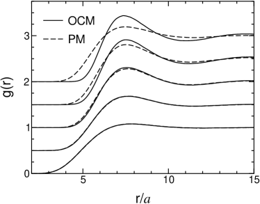
Figure 1: Macroion-macroion pair distribution function $g(r)$ vs. radial distance $r$ (units of macroion radius $a$) of salt-free suspensions computed from Monte Carlo simulations of the one-component model (OCM) with implicit counterions (solid curves) and the primitive model (PM) linse00 with explicit counterions (dashed curves) for macroion valence $Z=40$, volume fraction $\eta=0.01$, and electrostatic coupling parameters $\Gamma=\lambda_{B}/a=$ 0.0222, 0.0445, 0.0889, 0.1779, 0.3558 (bottom to top). For clarity, curves are vertically offset in steps of 0.5.

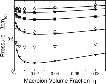
Figure 2: Reduced pressure $\beta p/n_{\rm tot}$ vs. macroion volume fraction $\eta$, where $n_{\rm tot}=(Z+1)n_{m}$, for salt-free suspensions computed from Monte Carlo simulations of the effective one-component model with implicit counterions (solid symbols) and the primitive model linse00 with explicit counterions (open symbols) for macroion valence $Z=40$ and several electrostatic coupling parameters $\Gamma=\lambda_{B}/a$. Simulation error bars are smaller than symbol sizes. Also shown are corresponding predictions of variational theory (curves). From top to bottom, $\Gamma=0.0222$, 0.0445, 0.0889, 0.1779, 0.3558.

At higher electrostatic couplings ($Z\lambda_{B}/a>7$), typical of highly charged latex particles and ionic surfactant micelles, significant deviations between the one-component and primitive models abruptly emerge ($\Gamma=0.3558$ in Figs. 1 and 2). The discrepancies in this relatively strong-coupling regime can be traced to renormalization of the effective macroion charge through strong association of counterions, a nonlinear effect neglected in the present version of the model. Preliminary investigations denton-lu-cr indicate, however, that the deviations can be substantially reduced by consistently building into the one-component model a renormalized effective charge. These results establish a threshold of $Z\lambda_{B}/a\simeq 7$ for significant charge renormalization within linear-response theory.

To test the variational free energy theory at higher charge asymmetries and nonzero salt concentrations, we compare predictions for the osmotic pressure (equation of state) with results from our GEMC simulations. The osmotic pressure, $\Pi=p-2n_{r}k_{B}T$, is here defined as the total pressure of the suspension less that of a (virtual) ideal-gas salt reservoir of ion pair density $n_{r}$ at the same salt chemical potential: $\mu_{s}=k_{B}T\ln(2n_{r}\Lambda_{\mu}^{3})$. Figure 3 shows sample results for the equation of state at fixed salt chemical potential or, equivalently, salt fugacity, $z_{s}=\exp(\beta\mu_{s}/2)$, from simulations at the salt concentrations predicted by theory for each volume fraction. Since theory and simulation assume identical effective interactions, the comparisons directly probe the excess free energy approximation [Eq. (11)] and corresponding pair potential contribution to the total pressure (inset to Fig. 3). The predictions are in excellent agreement with simulation over a wide range of volume fractions, further validating the variational approximation and providing a consistency check on our calculations. As an independent check, our methods accurately reproduce pressures computed from MC simulations of the hard-sphere-repulsive-Yukawa pair potential fluid cochran-chiew04 .

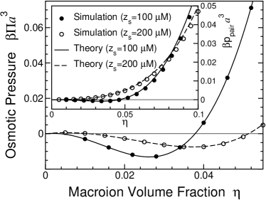
Figure 3: Reduced osmotic pressure $\beta\Pi a^{3}$ vs. volume fraction $\eta$ computed from Monte Carlo simulations and variational theory denton06 of the one-component model for Bjerrum length $\lambda_{B}=0.72$ nm, macroion radius $a=50$ nm, valence $Z=500$, and salt fugacities $z_{s}=100$ and 200 $\mu$M. Changes of curvature reflect phase instability. Inset: Pair potential contribution to total pressure. Simulation error bars are smaller than symbol sizes.

The appearance in Fig. 3 of a van der Waals loop in the pressure signals a spinodal instability and separation into macroion-rich (liquid) and macroion-poor (vapor) phases. We stress, however, that currently available data from primitive model simulations can test the effective one-component model and linearized effective interactions only for salt-free suspensions at relatively low charge asymmetries, where instabilities with respect to phase separation have not been predicted. Furthermore, the macroion aggregation observed in ref. linse00 in the strong-coupling regime is likely driven by microion correlations, which are neglected in the mean-field effective interactions assumed here. While further tests of the one-component model are needed, the close agreement for parameters accessible to primitive model simulations motivates proceeding to consider phase behavior.

V.2 Phase Behavior

To systematically map out the fluid binodal, we performed a series of GEMC simulations over ranges of volume fraction and salt concentration for selected macroion radii and valences: ($a=10$ nm, $Z=150$) and ($a=50$ nm, $Z=500$). Initially uniform systems of $N_{m}=500$ particles (two-box total), in thermodynamic states ($\eta$, $c_{s}$) within the predicted unstable region denton06 , spontaneously separated into two phases, each phase occupying one of the boxes, which differed in average macroion and salt densities. In contrast, systems at state points outside of the unstable region remained uniform. A visual impression of the phase separation is provided by the simulation snapshot in Fig. 4.

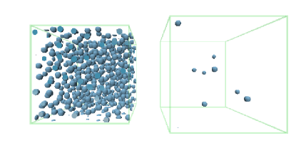
Figure 4: Snapshot from Gibbs ensemble Monte Carlo simulation, showing the two boxes after separation into macroion-rich and macroion-poor phases. Spheres depict macroions in the effective one-component model.

To identify the structure of the coexisting phases, we performed constant-$NVT$ (one-box) simulations, at identical state points, for particle numbers commensurate with likely crystal structures: fcc ($N_{m}=500$) and bcc ($N_{m}=432$). Initializing the particles on the sites of the respective lattice, we computed the equilibrium pair distribution function and observed typical fluid-like structure, indicating melting of the initial crystal. Upon increasing the volume fraction, we observed, at state points well outside the fluid binodal, an abrupt sharpening of the peaks of $g(r)$, reflecting crystallization. These observations are consistent with a simple hard-sphere freezing criterion, $\eta(d/2a)^{3}\simeq 0.49$, which approximates the macroions as hard spheres of effective diameter $d$ [from Eq. (11)] and locates the coexistence densities within the fluid regime.

The resulting phase diagrams are presented in Fig. 5, alongside predictions of variational theory denton06 , where tie lines joining corresponding points on the macroion-rich and macroion-poor binodal branches parallel those predicted by theory. Each pair of points on the binodal was produced by averaging over 10 independent runs, which differed only in the random number seed used for trial moves. Reported error bars represent statistical uncertainties of one standard deviation, computed from fluctuations in average densities among the 10 runs. Resolution near the critical point is blurred by density fluctuations and phase switching between boxes – a known limitation of the Gibbs ensemble method frenkel01 . For simplicity, we discarded runs in which the phases switched boxes, a rare occurrence away from the critical point. Considering the sensitivity of the coexistence analysis to slight deviations in free energy, the quantitative agreement between theory and simulation attests to the accuracy of the variational approximation.

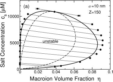
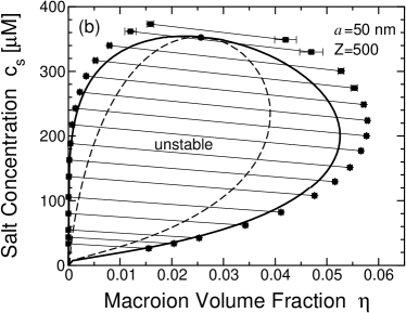
Figure 5: Phase diagrams of aqueous charged colloids, showing fluid binodal computed from Gibbs ensemble Monte Carlo simulations (squares) and variational theory denton06 (solid curves) for the effective one-component model at various combinations of macroion radius $a$ and valence $Z$. Tie lines join corresponding points on the colloid-rich and colloid-poor branches of the binodal. Also shown are predictions of variational theory for the critical point (circles) and spinodal (dashed curves).

Diagnostic variables were monitored during the simulations and evolved as typified by Fig. 6, which tracks the volume fractions, salt concentrations, pressures, and chemical potentials in each box vs. number of MC cycles for one sample run. Bifurcation of volume fractions and salt concentrations in the two boxes [Fig. 6 (a)] signals phase separation, while convergence of pressures and chemical potentials [Fig. 6 (b) and (c)] confirms equilibration. Several runs for larger systems (up to 1000 macroions) were performed to establish the insignificance of finite-size effects. Compared with large-scale simulations of the primitive model, our simulations require relatively modest computing resources, each run typically consuming 50-90 CPU hours on a single PC (Intel Xeon-HT processor).

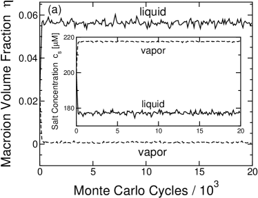
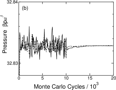
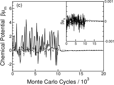
Figure 6: Evolution of diagnostic properties during a sample Gibbs ensemble Monte Carlo run for macroion radius $a=50$ nm, valence $Z=500$, total volume fraction $\eta=0.025$, and total salt concentration $c_{s}=200$ $\mu$M. Solid and dashed curves represent the two boxes. (a) volume fractions and (inset) salt concentrations; (b) total pressure; (c) macroion and (inset) salt chemical potentials, shifted to zero average. Instantaneous values are plotted during equilibration (first $10^{4}$ cycles) and cumulative values thereafter.

It should be emphasized that the observed phase separation, although perhaps surprising in the face of purely repulsive pair interactions, is driven by the state dependence of the volume energy in the one-component model of deionized suspensions. It is also important to note that the macroion valences and electrostatic couplings represented in Fig. 5 were selected to lie just within the unstable fluid regime and correspond to $\Gamma=$ 0.072 and 0.014 ($Z\lambda_{B}/a=$ 7 and 11) in panels (a) and (b), respectively (cf. $Z\lambda_{B}/a\simeq$ 1-14 in ref. linse00 ). In each case, a small increase in macroion radius or decrease in valence stabilizes the system. These parameters approach the threshold for charge renormalization estimated from our direct comparisons with primitive model simulations (Figs. 1 and 2), albeit for lower valences. Whether the predicted phase instability corresponds to a real phenomenon or is merely an artifact of the linearization approximation vongrunberg01 ; deserno02 ; tamashiro03 , or the assumption of fixed macroion valence levin98 ; levin01 ; levin03 ; levin04 ; zoetekouw_prl06 , remains unclear. Preliminary explorations denton-lu-cr , based on a simple model of effective macroion valence, suggest that the instability survives incorporation of charge renormalization in the one-component model. Further studies are required, however, to resolve this important issue.

VI Conclusions

In summary, we have developed a new variant of the Gibbs ensemble Monte Carlo method to simulate a one-component model of charged colloids governed by density-dependent effective interactions. The effective interactions (pair potential and one-body volume energy) are input from linear-response theory, assuming a mean-field approximation for microion structure. The simulation algorithm includes trial exchanges of implicit salt between the two simulation boxes and incorporates the volume energy into the acceptance probabilities for trial moves that change the average macroion or salt density.

Comparisons with simulations of the two-component (salt-free) primitive model linse00 demonstrate the validity of the one-component model over a wide parameter range, physically relevant to charged latex particles and micelles. Results for the macroion-macroion pair distribution function and pressure are in close agreement with corresponding primitive model results for moderate electrostatic couplings. Deviations at stronger couplings likely originate from nonlinear screening effects neglected in the present model. Our simulations also confirm the accuracy of a variational free energy approximation vRH97 ; vRDH99 ; vRE99 ; denton06 . Further comparisons would help to more sharply define the limitations of the one-component model.

While the cost of primitive model simulations grows with increasing charge asymmetry, concentration, and electrostatic coupling, the computational effort required to simulate the one-component model is relatively modest and actually diminishes with increasing macroion valence and concentration, as decreasing the screening length shortens the range of effective pair interactions. The one-component model thus offers insight into bulk phase behavior in parameter regimes that may be computationally prohibitive for more explicit models.

We have applied our new simulation method to test predictions of variational theory denton06 for the phase behavior of aqueous suspensions of charged macroions with weakly correlated (monovalent) microions at low salt concentrations. The resulting phase diagrams exhibit coexistence of macroion-rich and macroion-poor fluid phases in excellent agreement with previous predictions and qualitatively consistent with observed thermodynamic anomalies. The phase instability predicted by theory, and now confirmed by simulations of the same model, occurs in a parameter regime that appears to border the threshold for saturation of the effective macroion charge. Future work will address this open issue by incorporating charge renormalization into the one-component model denton-lu-cr . Finally, our simulation algorithm can be extended to investigate other phase transitions, e.g., crystallization, and adapted to model other soft materials, such as polyelectrolyte and ionic micellar solutions.

Appendix A Diagnostic Calculations

A.1 Pressure

A diagnostic for mechanical equilibrium in the Gibbs ensemble is equality of pressures in the two boxes. The total pressure naturally separates into three distinct contributions:

$$p=p_{\rm id}+p_{\rm pair}+p_{\rm vol},$$ (18)

where $p_{\rm id}=\left\langle n_{m}\right\rangle k_{B}T$ is the ideal-gas pressure of the macroions, $p_{\rm pair}$ results from effective pair interactions between macroions, $p_{\rm vol}=-\left\langle(\partial E_{\rm vol}/\partial V)_{N_{m}/N_{s}}\right\rangle$ is the contribution from the density-dependent volume energy, and angular brackets denote an ensemble average over configurations in the Gibbs ensemble. The pair pressure is calculated on the fly within the simulations using the virial expression for a density-dependent pair potential louis02 :

$$p_{\rm pair}=\left\langle\frac{{\cal V}_{\rm int}}{3V}\right\rangle-\left\langle\left(\frac{\partial U_{\rm pair}}{\partial V}\right)_{N_{m}/N_{s}}\right\rangle+p_{\rm tail},$$ (19)

where ${\cal V}_{\rm int}$ is the internal virial, the volume derivative term accounts for the density dependence of the effective pair potential, and $p_{\rm tail}$ corrects for cutting off the long-range tail of the pair potential. The internal virial is given by

$${\cal V}_{\rm int}=\sum_{i=1}^{N_{m}}{\bf r}_{i}\cdot{\bf f}_{i}=\sum_{i\neq j=1}^{N_{m}}(1+\kappa r_{ij})v_{\rm eff}(r_{ij}),$$ (20)

where ${\bf f}_{i}=-\nabla\sum_{j\neq i}v_{\rm eff}(r_{ij})$ is the effective force exerted on macroion $i$, at position ${\bf r}_{i}$, by all neighboring macroions $j$, at relative distances $r_{ij}$, within the cut-off radius $r_{c}$. The second term on the right side of Eq. (19) is computed via

$$\left(\frac{\partial U_{\rm pair}}{\partial V}\right)_{N_{s}/N_{m}}=-\frac{n_{m}^{2}}{2N_{m}}\sum_{i\neq j=1}^{N_{m}}\left(\frac{\partial v_{\rm eff}(r_{ij})}{\partial n_{m}}\right)_{N_{s}/N_{m}}$$ (21)

with

$$\left(\frac{\partial v_{\rm eff}(r)}{\partial n_{m}}\right)_{N_{s}/N_{m}}=\left(\frac{\kappa^{2}a^{2}}{1+\kappa a}-\frac{\kappa r}{2}\right)\frac{v_{\rm eff}(r)}{n_{m}(1-\eta)}.$$ (22)

The tail pressure is approximated by

$$p_{\rm tail} = -\frac{2\pi}{3}\left\langle n_{m}^{2}\int_{r_{c}}^{\infty}{\rm d}r\,r^{3}v^{\prime}_{\rm eff}(r)\right\rangle$$

$$= \frac{2\pi}{3}\left\langle n_{m}^{2}\left(\frac{\kappa^{2}r_{c}^{2}+3\kappa r_{c}+3}{\kappa^{2}}\right)r_{c}v_{\rm eff}(r_{c})\right\rangle,$$

the approximation being the neglect of pair correlations for $r>r_{c}$. Finally, the volume pressure is given by

$$\beta p_{\rm vol}=\left\langle\frac{n_{m}}{1-\eta}\left(Z+2\frac{N_{s}}{N_{m}}-\frac{Z^{2}\kappa\lambda_{B}}{4(1+\kappa a)^{2}}\right)\right\rangle.$$ (24)

A.2 Chemical Potentials

To diagnose chemical equilibrium between coexisting phases, we computed the chemical potentials of macroions and salt by adapting Widom’s test particle insertion method widom63 to the Gibbs ensemble, following ref. frenkel01 . In contrast to the original method, the inserted ions are not treated as ghost particles in GEMC, but rather remain within the box into which they are successfully transferred. The macroion chemical potential – the change in Helmholtz free energy upon adding a macroion – can be expressed as

$$\mu_{m}=-k_{B}T\ln\left(\frac{{\cal Z}_{G}(N_{m}+1,N_{s},V,T)}{{\cal Z}_{G}(N_{m},N_{s},V,T)}\right),$$ (25)

where the Gibbs ensemble partition function is given by

$${\cal Z}_{G} = \frac{1}{\Lambda^{3N_{m}}V}\sum_{N_{m1}=0}^{N_{m}}\frac{1}{N_{m1}!(N_{m}-N_{m1})!}$$ (26)

$$\times \int_{0}^{V}{\rm d}V_{1}\,V_{1}^{N_{m1}}(V-V_{1})^{N_{m}-N_{m1}}$$

$$\times \int{\rm d}{\bf s}^{N_{m}}\,\exp[-\beta U(\{{\bf s}\};n_{m},n_{s})].$$

The macroion chemical potential of box 1 is thus computed from frenkel01

$$\mu_{m1}=-k_{B}T\ln\left\langle\frac{V_{1}/\Lambda^{3}}{(N_{m1}+1)}\exp(-\beta\Delta U_{1}^{+m})\right\rangle,$$ (27)

where $\Delta U_{1}^{+m}=U(N_{m1}+1)-U(N_{m1})$ is the change in total potential energy (volume energy plus pair energy) of box 1 upon insertion of a macroion. In practice, the large change in volume energy $\Delta E_{\rm vol}$ resulting from a macroion insertion necessitates evaluating Eq. (27) by adding to and subtracting from the argument of the exponential a constant $c\simeq\left\langle\Delta E_{\rm vol}\right\rangle$:

$$\mu_{m1} = -k_{B}T\ln\left\langle\frac{V_{1}/\Lambda^{3}}{N_{m1}+1}\exp[-\beta(\Delta U_{1}^{+m}-c~{})]\right\rangle$$ (28)

$$+ c.$$

The salt chemical potential – the change in Helmholtz free energy upon insertion of a salt ion pair – can be approximated by

$$\mu_{s}=-\frac{k_{B}T}{\Delta N_{s}}\ln\left(\frac{{\cal Z}_{G}(N_{m},N_{s}+\Delta N_{s},V,T)}{{\cal Z}_{G}(N_{m},N_{s},V,T)}\right),$$ (29)

assuming that the number of exchanged salt ion pairs $\Delta N_{s}$ is much less than the total number of salt ion pairs ($\Delta N_{s}\ll N_{s}$). The salt chemical potential of box 1 is thus computed from

$$\mu_{s1}=-\frac{k_{B}T}{\Delta N_{s}}\ln\left\langle\exp[-\beta(\Delta U_{1}^{+s}-c~{})]\right\rangle+\frac{c}{\Delta N_{s}},$$ (30)

where $\Delta U_{1}^{+s}=U(N_{s1}+\Delta N_{s})-U(N_{s1})$ is the change in total potential energy of box 1 upon insertion of $\Delta N_{s}$ salt ion pairs. The absence of combinatorial and phase space factors in Eq. (30) follows from modeling the microions only implicitly. Note also that the chemical potentials are defined only to within arbitrary constants. In the dilute colloid limit ($N_{m}\to 0$), the salt chemical potential tends to that of an ideal gas of salt ions

$$\mu_{s}^{(0)}=2k_{B}T\left\langle\ln(n_{s}\Lambda_{\mu}^{3})\right\rangle$$ (31)

and the macroion chemical potential reduces to

$$\mu_{m}^{(0)} = k_{B}T\left\langle-\ln\left(\frac{V}{\Lambda^{3}}\right)+Z\ln(n_{s}\Lambda_{\mu}^{3})\right.$$ (32)

$$- \left.\phantom{\int}\left(\frac{Z}{z}\right)^{2}\frac{\kappa\lambda_{B}}{2(1+\kappa a)}+\frac{8\pi}{3}n_{s}a^{3}\right\rangle,$$

where the terms on the right side are derived (left to right) from the macroion entropy, microion entropy, macroion-counterion interaction, and macroion excluded volume. These analytical results [Eqs. (31) and (32)] provide a check on the numerical results in the limit in which one box becomes depleted of macroions.

A.3 Pair Distribution Function

The structure of the suspension is characterized by the pair distribution functions HM . The macroion-macroion pair distribution function $g(r)$ – the only one accessible in the one-component model – is defined such that $4\pi r^{2}g(r){\rm d}r$ equals the average number of macroions in a spherical shell of radius $r$ and thickness ${\rm d}r$ centered on a macroion. For a given configuration, each particle is regarded, in turn, as the central particle. Neighboring particles are then assigned, according to their radial distance $r$ from the central particle, to concentric spherical shells (bins) of thickness $\Delta r=0.1a$. After equilibration, $g(r)$ is computed, in the range $2a<r<L/2$, by accumulating the numbers of particles in radial bins and averaging over all configurations. The resulting distributions are finally smoothed by averaging each bin with its immediate neighboring bins.

References

- (1) P. N. Pusey, in Liquids, Freezing and Glass Transition, session 51, ed. J.-P. Hansen, D. Levesque, and J. Zinn-Justin (North-Holland, Amsterdam, 1991).
- (2) B. V. R. Tata, M. Rajalakshmi, and A. K. Arora, Phys. Rev. Lett. 69, 3778 (1992).
- (3) K. Ito, H. Yoshida, and N. Ise, Science 263, 66 (1994).
- (4) N. Ise and H. Yoshida, Acc. Chem. Res. 29, 3 (1996).
- (5) B. V. R. Tata, E. Yamahara, P. V. Rajamani, and N. Ise, Phys. Rev. Lett. 78, 2660 (1997).
- (6) N. Ise, T. Konishi, and B. V. R. Tata, Langmuir 15, 4176 (1999).
- (7) H. Matsuoka, T. Harada, and H. Yamaoka, Langmuir 10, 4423 (1994); H. Matsuoka, T. Harada, K. Kago, and H. Yamaoka, ibid 12, 5588 (1996); T. Harada, H. Matsuoka, T. Ikeda, and H. Yamaoka, ibid 15, 573 (1999).
- (8) F. Gröhn and M. Antonietti, Macromolecules 33, 5938 (2000).
- (9) A. E. Larsen and D. G. Grier, Nature 385, 230 (1997).
- (10) B. V. Derjaguin and L. Landau, Acta Physicochimica (USSR) 14, 633 (1941).
- (11) E. J. W. Verwey and J. T. G. Overbeek, Theory of the Stability of Lyophobic Colloids (Elsevier, Amsterdam, 1948).
- (12) R. van Roij and J.-P. Hansen, Phys. Rev. Lett. 79, 3082 (1997).
- (13) R. van Roij, M. Dijkstra, and J.-P. Hansen, Phys. Rev. E 59, 2010 (1999).
- (14) R. van Roij and R. Evans, J. Phys.: Condens. Matter 11, 10047 (1999).
- (15) B. Zoetekouw and R. van Roij, Phys. Rev. E 73, 21403 (2006).
- (16) P. B. Warren, J. Chem. Phys. 112, 4683 (2000); J. Phys.: Condens. Matter 15, S3467 (2003); Phys. Rev. E 73, 011411 (2006).
- (17) B. Beresford-Smith, D. Y. C. Chan, and D. J. Mitchell, J. Coll. Int. Sci. 105, 216 (1985).
- (18) D. Y. C. Chan, P. Linse, and S. N. Petris, Langmuir 17, 4202 (2001).
- (19) M. J. Grimson and M. Silbert, Mol. Phys. 74, 397 (1991).
- (20) A. R. Denton, J. Phys.: Condens. Matter 11, 10061 (1999).
- (21) A. R. Denton, Phys. Rev. E 62, 3855 (2000).
- (22) A. R. Denton, Phys. Rev. E 70, 31404 (2004).
- (23) A. R. Denton, Phys. Rev. E 73, 041407 (2006).
- (24) J.-P. Hansen and H. Löwen, Annu. Rev. Phys. Chem. 51, 209 (2000).
- (25) L. Belloni, J. Phys.: Condens. Matter 12, R549 (2000).
- (26) Y. Levin, Rep. Prog. Phys. 65, 1577 (2002).
- (27) H. H. von Grünberg, R. van Roij, and G. Klein, Europhys. Lett. 55, 580 (2001).
- (28) M. Deserno, H. H. von Grünberg, Phys. Rev. E 66, 011401 (2002).
- (29) M. N. Tamashiro and H. Schiessel, J. Chem. Phys. 119, 1855 (2003).
- (30) Y. Levin, M. C. Barbosa, and M. N. Tamashiro, Europhys. Lett. 41, 123 (1998).
- (31) A. Diehl, M. C. Barbosa, and Y. Levin, Europhys. Lett. 53, 86 (2001).
- (32) Y. Levin, E. Trizac, and L. Bocquet, J. Phys.: Condens. Matter 15, S3523 (2003).
- (33) A. Diehl and Y. Levin, J. Chem. Phys. 121, 12100 (2004).
- (34) B. Zoetekouw and R. van Roij, Phys. Rev. Lett. 97, 258302 (2006).
- (35) P. Linse, J. Chem. Phys. 113, 4359 (2000).
- (36) A.-P. Hynninen, M. Dijkstra, and A. Z. Panagiotopoulos, J. Chem. Phys. 123, 84903 (2005).
- (37) J. Liu and E. Luijten, Phys. Rev. Lett. 92, 35504 (2004).
- (38) J.-P. Hansen and I. R. McDonald, Theory of Simple Liquids, ed. (Academic, London, 1986).
- (39) J. S. Rowlinson, Mol. Phys. 52, 567 (1984).
- (40) A. Z. Panagiotopoulos, J. Phys.: Condens. Matter 12, R25 (2000).
- (41) A. Z. Panagiotopoulos, Mol. Phys. 61, 813 (1987).
- (42) A. Z. Panagiotopoulos, N. Quirke, M. Stapleton, and D. J. Tildesley Mol. Phys. 63, 527 (1988).
- (43) A. Z. Panagiotopoulos, Int. J. Thermophys. 4, 739 (1989).
- (44) A. Z. Panagiotopoulos, in Observation, Prediction, and Simulation of Phase Transitions in Complex Fluids, NATO ASI Series C 460 463, ed. M. Baus, L. R. Rull, and J. P. Ryckaert (Dordrecht, Kluwer, 1995).
- (45) B. Smit, T. Hauschild, and J. M. Prausnitz, Mol. Phys. 77, 1021 (1992).
- (46) N. Metropolis, A. W. Rosenbluth, M. N. Rosenbluth, A. H. Teller, and E. Teller, J. Chem. Phys. 21, 1087 (1953).
- (47) D. Frenkel and B. Smit, Understanding Molecular Simulation (London, Academic, 2001).
- (48) M. P. Allen and D. J. Tildesley, Computer Simulation of Liquids (Oxford, Oxford, 1987).
- (49) Reduced pressures in Table III of ref. linse00 should be for , , ; 0.970 for , , ; and 0.971 for , , (P. Linse, private communication).
- (50) A. R. Denton and B. Lu, unpublished.
- (51) T. W. Cochran and Y. C. Chiew, J. Chem. Phys. 121, 1480 (2004).
- (52) A. A. Louis, J. Phys.: Condens. Matter 14, 9187 (2002).
- (53) B. J. Widom, J. Chem. Phys. 39, 2808 (1963).