On the Limiting Cases of Nonextensive Thermostatistics

Abstract

We investigate the limiting cases of Tsallis statistics. The viewpoint adopted is not the standard information-theoretic one, where one derives the distribution from a given measure of information. Instead the mechanical approach recently proposed in [M. Campisi, G.B. Bagci, Phys. Lett. A (2006), doi:10.1016/j.physleta.2006.09.081], is adopted, where the distribution is given and one looks for the associated physical entropy. We show that, not only the canonical ensemble is recovered in the limit of $q$ tending to one, as one expects, but also the microcanonical ensemble is recovered in the limit of $q$ tending to minus infinity. The physical entropy associated with Tsallis ensemble recovers the microcanonical entropy as well and we note that the microcanonical equipartition theorem is recovered too. We are so led to interpret the extensivity parameter q as a measure of the thermal bath heat capacity: $q=1$ (i.e. canonical) corresponds to an infinite bath (thermalised case, temperature is fixed), $q=-\infty$ (microcanonical) corresponds to a bath with null heat capacity (isolated case, energy is fixed), intermediate $q^{\prime}s$ (i.e. Tsallis) correspond to the realistic cases of finite heat capacity (both temperature and energy fluctuate).

It is a very well known fact that nonextensive thermostatistics, based on q-exponential power-law ensembles generalizes the standard statistical mechanics stemming from the canonical ensemble, to which it tends as the non-extensive parameter $q$ approaches 1. This generalization has been first proposed within an information-theoretic approach where the standard Shannon-Gibbs entropy is replaced by the order-q Tsallis entropy. As $q$ approaches 1, the Tsallis entropy approaches Shannon-Gibbs entropy and one is able to recover standard statistical mechanics Tsallis (1988). Very recently a new approach has been proposed to study the theoretical foundations of nonextensive thermostatistics Campisi and Bagci (2006). This approach is based on the concept of “orthode” originally proposed by Boltzmann in the 1880s and is completely independent from the information-theoretic one Gallavotti (1995). The approach provides a criterion to assess whether a given statistical ensemble provides a “mechanical model of thermodynamics”, and, if this is the case, tells what is the physical entropy associated to a given ensemble. In this respect the method proceeds along the opposite path followed in the information-theoretic approach where, instead, one starts from an entropy function and derives the ensemble. In a previous work Campisi and Bagci (2006) we have shown that the Tsallis ensemble:

$$\rho_{q}(\textbf{z};U,V)=\frac{\left[1-\beta(1-q)(H(\textbf{z};V)-U)\right]^{\frac{q}{1-q}}}{N_{q}},$$ (1)

where

$$N_{q}(U,V)=\int d\textbf{z}\left[1-(1-q)\beta(H(\textbf{z};V)-U)\right]^{\frac{q}{1-q}},$$ (2)

is an “orthode”, namely it provides a mechanical model of thermodynamics in the sense mentioned above. Within such a mechanical approach the entropy is given by the $1/q$-order Rényi information associated with the distribution $\rho_{q}$ :

$$S^{[q]}(U,V)=\log\int d\textbf{z}\left[1-(1-q)\beta(H(\textbf{z};V)-U)\right]^{\frac{1}{1-q}}$$ (3)

This entropy is consistent with the maximum information-entropy principle Campisi and Bagci (2006); Bashkirov (2004) and can be considered as a good expression for the physical entropy Campisi and Bagci (2006). As we shall see, when $q$ tends to 1, the distribution (1) tends to the canonical distribution and the entropy (3) tends to the canonical entropy. In sum the Tsallis ensemble provides a mechanical generalization of canonical ensemble. The main result of the present work is that the same ensemble can be seen as a generalization of the microcanonical ensemble as well, to which it reduces when the index $q$ tends to minus infinity. We shall also provide a physical interpretation for the generalization scheme where canonical and microcanonical ensemble represent two limiting cases.

According to Boltzmann’s reasoning, one family (i.e., ensemble) of distributions, $\rho(\mathbf{z};\lambda_{i})$ parameterized by a given number of parameters $\lambda_{i}$, provides a mechanical model of thermodynamics, i.e., it is an orthode if, defined the macroscopic state of the system by the set of following quantities:

$$U_{\rho}=\left\langle H\right\rangle_{\rho}$$ “energy”

 “doubled kinetic energy per degree of freedom”

 “generalized displacement”

 “generalized conjugated force”,

(4)

for infinitesimal and independent changes of the $\lambda_{i}$’s, the heat theorem

$$\frac{dU_{\rho}+P_{\rho}dV_{\rho}}{T_{\rho}}=exact\quad differential$$ (5)

holds Gallavotti (1995); Campisi (2005). In sum the ensemble provides a mechanical model of thermodynamics if the average of certain mechanical quantities evaluated over the ensemble’s distributions are related to each other according to the fundamental equation of thermodynamics. If this is the case, the quantity that generates the differential is to be interpreted as the physical entropy associated with the given ensemble.

For example the canonical ensemble, which is parameterized by $(\beta,V)$, reads:

$$\rho_{c}(\mathbf{z};\beta,V)=\frac{e^{-\beta H(\mathbf{z};V)}}{Z(\beta,V)}$$ (6)

where

$$Z(\beta,V)=\int d\textbf{z}e^{-\beta H(\mathbf{z};V)}$$ (7)

The corresponding entropy is given by the well known formula:

$$S_{c}(\beta,V)=\beta U_{c}(\beta,V)+\log Z(\beta,V)$$ (8)

To see that this function generates the heat differential, it is enough to take the partial derivatives of $S_{c}$ and use the canonical equipartition theorem:

$$T_{c}=\left\langle p_{i}\frac{\partial H}{\partial p_{i}}\right\rangle_{c}=\frac{1}{\beta}$$ (9)

where the symbol $<\cdot>_{c}$ denotes average over the canonical distribution (6).

Similarly the microcanonical ensemble, which is parameterized by $(U,V)$, reads:

$$\rho_{mc}(\mathbf{z};U,V)=\frac{\delta(U-H(\mathbf{z};V))}{\Omega(U,V)}$$ (10)

where

$$\Omega(U,V)=\int d\mathbf{z}\delta(U-H(\mathbf{z};V))$$ (11)

denotes the structure function Khinchin (1949). As shown in Ref. Campisi (2005) the corresponding entropy is given by

$$S_{mc}(U,V)=\log\int d\mathbf{z}\theta(U-H(\mathbf{z};V))$$ (12)

To see that this is the right entropic function it is enough to take the partial derivatives and use the microcanonical equipartition theorem Khinchin (1949):

$$T_{mc}=\left\langle p_{i}\frac{\partial H}{\partial p_{i}}\right\rangle_{mc}=\frac{\Omega(U,V)}{\Phi(U,V)}$$ (13)

where $<\cdot>_{mc}$ denotes average over the microcanonical distribution (10) and

$$\Phi(U,V)=\int d\mathbf{z}\theta(U-H(\mathbf{z};V)).$$ (14)

As the work of Ref. Campisi and Bagci (2006) has highlighted, a completely similar situation occurs for the ensemble (1), and the entropy (3). Namely the work of Ref. Campisi and Bagci (2006) has shown that the Tsallis ensemble of Eq. (1) is an orthode too. The same work also suggested that the Tsallis ensemble can be considered as a hybrid ensemble. This refers to the fact that both $\beta$ and $U$, appear explicitly in its expression, therefore one can choose between two possible parameterizations: either fixes $U$ and adjusts $\beta$ in such a way that

$$U=\left\langle H\right\rangle,$$ (15)

or, fixes $\beta$ and adjusts $U$, in such a way that the same equation be satisfied (throughout this paper, the symbol $<\cdot>$ denotes average over Tsallis ensemble (1)). In the first case one has $\beta=\beta(U,V)$, and the ensemble will be parameterized by $(U,V)$, in the second $U=U(\beta,V)$, and the parameters will be $(\beta,V)$. In sum, there is a duality, between two possible representations: the microcanonical-like one and the canonical-like one. So, according to the parametrization adopted, one can see the Tsallis ensemble either as a generalized canonical ensemble or as a generalized microcanonical ensemble. This is true not only from a qualitative viewpoint, but also from a quantitative one. As it is well known, the ensemble (1) is indeed a generalization of the canonical one to which it tends when $q$ goes to $1$. In fact, for the well-known properties of the $q$-exponential Tsallis et al. (1998), we have:

$$\lim_{q\rightarrow 1}\rho_{q}=\frac{e^{-\beta H}}{Z}=\rho_{c},\qquad\lim_{q\rightarrow 1}S^{[q]}=\beta U+\log Z=S_{c}$$ (16)

We would like to stress that, in this limit the explicit dependence of the distribution $\rho_{q}$ on $U$ disappears. Namely the duality property is lost in the limit $q\rightarrow 1$, as the only possible parametrization is the $(\beta,V)$ one.

In a similar manner the microcanonical orthode is a special case of Tsallis orthode recovered in the limit $q\rightarrow-\infty$, in which case the explicit dependence on $\beta$ disappears. In this limit, again, the duality is lost and the only possible parametrization is the $(U,V)$ one. Considering the q-exponential function:

$$e_{q}(x)=\left\{\begin{tabular}[]{ll}0&$1+(1-q)x<0$\\ $\left[1+(1-q)x\right]^{1/(1-q)}$&$1+(1-q)x\geq 0$\\ \end{tabular}\right.$$ (17)

it is easily seen that:

$$\lim_{q\rightarrow-\infty}e_{q}(x)=\left\{\begin{tabular}[]{ll}0&$x<0$\\ 1&$x\geq 0$\end{tabular}\right.=\theta(x).$$ (18)

This fact is illustrated in Figure 1.

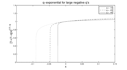
Figure 1: Plot of q-exponential (Eq. 17) for large negative values of $q$. The function tends to the Heaviside step function.

Therefore one has

$$\lim_{q\rightarrow-\infty}S^{[q]}=S_{mc}$$ (19)

where we have used the fact that $\theta(\beta x)=\theta(x)$ for $\beta>0$. Further one has that the Tsallis ensemble (1) is expressed in terms of the “derivative” of the q-exponential

$$e^{\prime}_{q}(x)=\left\{\begin{tabular}[]{ll}0&$1+(1-q)x<0$\\ $\left[1+(1-q)x\right]^{q/(1-q)}$&$1+(1-q)x\geq 0$\\ \end{tabular}\right.$$ (20)

which tends to a Dirac delta function. This is graphically illustrated in Fig. 2.

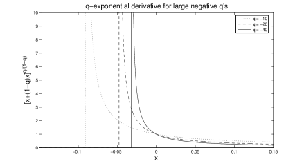
Figure 2: Plot of q-exponential derivative (Eq. 20) for large negative values of $q$. The function approaches a Dirac delta function.

A simple way to prove this result is to consider the Fourier transform of the function $e^{\prime}_{q}$:

$$\widehat{e^{\prime}_{q}}(\omega)=e^{-i\omega\alpha_{q}}\frac{\Gamma(\alpha_{q}+1)}{(-i\omega\alpha_{q})^{\alpha_{q}}}$$ (21)

where for simplicity we have used the notation $\alpha_{q}=1/(1-q)$. Now it is easily seen that, in the limit $q\rightarrow-\infty$ ($\alpha_{q}\rightarrow 0^{+}$), $\widehat{e^{\prime}_{q}}(\omega)\rightarrow 1$ which is the Fourier transform of the Dirac delta. Therefore the function $e^{\prime}_{q}(x)$ tends to the delta function. From this it follows that the distribution $\rho_{q}$ tends to the microcanonical distribution:

$$\lim_{q\rightarrow-\infty}\rho_{q}=\frac{\delta(U-H(\textbf{z};V))}{\int\delta(U-H(\mathbf{z};V))}=\rho_{mc}$$ (22)

It is evident that, due to the property $\delta(\beta x)=\beta^{-1}\delta(x)$, in the limit $q\rightarrow-\infty$, the explicit dependence on $\beta$ disappeared. This is understood also based on the fact that, being the distribution extremely peaked, the average of $H$ always equals $U$, no matter the value taken by $\beta$.

It is important to notice that the microcanonical equipartition theorem is recovered too. The equipartition theorem associated with the ensemble (1), reads Martínez et al. (2002):

$$T^{[q]}=\left\langle p_{i}\frac{\partial H}{\partial p_{i}}\right\rangle=\frac{1}{\beta}\frac{N_{q}}{\mathcal{N}_{q}}$$ (23)

where:

$$\mathcal{N}_{q}(U,V)=\int d\textbf{z}\left[1-(1-q)\beta(H(\textbf{z};V)-U)\right]^{\frac{1}{1-q}}$$ (24)

For finite q’s, thanks to Eq. (15), we have $N_{q}=\mathcal{N}_{q}$ hence $T^{[q]}=\frac{1}{\beta}$ Martínez et al. (2002). Therefore the canonical equipartition theorem (see Eq. 9) is trivially recovered for $q=1$. Nonetheless, when $q$ goes to infinity, the relation $N_{q}=\mathcal{N}_{q}$ stops holding. In facts we have

$$\lim_{q\rightarrow-\infty}\mathcal{N}_{q}=\Phi\qquad\lim_{q\rightarrow-\infty}N_{q}=\frac{1}{\beta}\Omega$$

so that $\lim_{q\rightarrow-\infty}T^{[q]}=\frac{\Omega}{\Phi}$, namely the microcanonical equipartition theorem is recovered as well.

Thanks to the mechanical approach of Boltzmann, we have been able to see how the microcanonical and canonical orthodes are two extremal cases of a more general family of hybrid orthodes, which can be parameterized either through $(U,V)$ or $(\beta,V)$. We shall refer to this fact as the $\beta\leftrightarrow U$ duality. The microcanonical and canonical ensembles arise as the two opposite limits where the duality property is lost.

We shall now investigate the physical meaning of such hybrid statistics. In other words, we shall ask ourselves in what physical situation we expect to observe Tsallis statistics. It is well known that the microcanonical ensemble describes the statistical properties of isolated systems whereas the canonical one well describes the properties of systems in contact with a heat bath. Both ensembles apply to two ideal (nonetheless very useful) cases: that of a system in contact with a heat bath with infinite capacity (the temperature is fixed) and that of an isolated system, namely a system in contact with a bath with null specific heat (the energy is fixed). Between these two extremal cases lie the physical realistic cases of systems in contact with finite heat baths, where both energy and temperature are allowed to fluctuate. Therefore we find it reasonable to expect such systems to obey Tsallis statistics of some order $q$, where $q$ accounts for the specific heat of the bath. The idea of finite heat bath is not new in the context of non-extensive thermodynamics. It was first proposed in Plastino and Plastino (1994), and then further developed in Almeida (2001), although the limiting case of null heat capacity was never investigated before. In particular Almeida Almeida (2001) considered an isolated system of total energy $a$ composed of two non interacting subsystems: the system of interest (labelled by the subscript $1$) and its complement, the bath (labelled by $2$). The total Hamiltonian splits in the sum of the two sub-system hamiltonians, $H=H_{1}+H_{2}$. Using the structure function of the total system ($\Omega$), and that of the bath ($\Omega_{2}$), one can express the distribution law for the component $1$, in its phase space as Khinchin (1949):

$$p_{1}(H_{1})=\frac{\Omega_{2}(a-H_{1})}{\Omega(a)}.$$ (25)

By defining the inverse temperature of the bath as $\beta_{2}\doteq\frac{\Omega^{\prime}_{2}}{\Omega_{2}}$, Almeida proved that the bath specific heat ($C_{V}^{-1}\doteq\frac{\partial}{\partial E_{2}}\frac{1}{\beta_{2}}$) is given by the expression $C_{V}=\frac{1}{1-q}$, if and only if:

$$\frac{\Omega_{2}(a-H_{1})}{\Omega_{2}(a)}=e_{q}(-\beta_{2}(a)H_{1})$$ (26)

namely, if and only if $p_{1}(H_{1})\propto e_{q}(-\beta_{2}(a)H_{1})$. Although this theorem is in line with our interpretation based on finite heat baths, it leads to a form of Tsallis distribution expressed in terms of $e_{q}$ rather than the form investigated here expressed in terms of $e^{\prime}_{q}$. The latter would correspond to the escort version of the former. As the reader can easily notice the microcanonical distribution is not a special case of the $e_{q}$-type distribution. At this point we notice that the definition $\beta_{2}\doteq\frac{\Omega^{\prime}_{2}}{\Omega_{2}}$ adopted by Almeida is not consistent with the microcanonical equipartition prescription (13). If one adopts the correct definition

$$\beta_{2}\doteq\frac{\Omega_{2}}{\Phi_{2}},$$ (27)

of bath’s temperature, namely if one replaces $\Omega_{2}$ with $\Phi_{2}$ then Almeida’s theorem would read: $C_{V}=\frac{1}{1-q}\Leftrightarrow\frac{\Phi_{2}(a-H_{1})}{\Phi_{2}(a)}=e_{q}(-\beta_{2}(a)H_{1})$. By taking the derivative of the latter with respect to $H_{1}$, we obtain the following:

Theorem 1

$$\frac{\Omega_{2}(a-H_{1})}{\Omega_{2}(a)}=e^{\prime}_{q}(-\beta_{2}(a)H_{1})$$ (28)

if and only if

$$C_{V}\doteq\left(\frac{\partial}{\partial E_{2}}\frac{1}{\beta_{2}}\right)^{-1}=\frac{1}{1-q}.$$ (29)

Now we notice that $\beta_{2}(a)$ is the inverse physical temperature that the bath would have if it were isolated and its energy were $a$. Thanks to Eq. (29) such temperature is given by $\frac{1}{\beta_{2}(a)}=(1-q)a$. Instead, in the physical situation under study, the bath is in contact with system $1$ and its average energy $U_{2}$ is smaller than $a$. The actual temperature in the composite system may be expressed by $\frac{1}{\beta}=(1-q)U_{2}$. Therefore $\beta(a)=\beta U_{2}/a$, hence Eq. (28) may be rewritten as $p_{1}(H_{1})\propto\left[1+\left(\frac{a}{U_{2}}-1\right)-(1-q)\beta H_{1}\right]^{\frac{q}{1-q}}$. Using the relation $a=U_{1}+U_{2}$ then $p_{1}$ would read exactly as the Tsallis distribution of Eq. (1).

In sum, the theorem says that if the heat capacity of the bath is $C_{V}=\frac{1}{1-q}$, then the component $1$ obeys Tsallis distribution law of Eq. (1) of index $q$. This theorem is consistent with our physical interpretation according to which $q$ should account for the finiteness of the bath specific heat. In particular it reproduces well the two limiting cases: if $q\rightarrow 1$ then $C_{V}$ goes to infinity, namely we are in the case of infinite bath, and accordingly we get the canonical ensemble. If $q\rightarrow-\infty$ then $C_{V}\rightarrow 0$, namely we are in the isolated case, and accordingly we get the microcanonical ensemble. Thanks to the theorem above and the nonextensive equipartition theorem ($T=\frac{1}{\beta}$), we are finally in the position to write the distribution law for system 1 in terms of physical quantities as:

$$\rho_{C_{V}}(\textbf{z};U,V)=\frac{\left[1-\frac{(H(\textbf{z};V)-U)}{C_{V}T}\right]^{C_{V}-1}}{N_{C_{V}}(U,V)},$$ (30)

where for simplicity we dropped the subscript 1. Accordingly its entropy would read:

$$S_{C_{V}}(U,V)=\log\int d\textbf{z}\left[1-\frac{(H(\textbf{z};V)-U)}{C_{V}T}\right]^{C_{V}}$$ (31)

In conclusion the main novelty of this work is that of pointing out that the microcanonical ensemble is a limiting case of Tsallis ensemble. This can be seen if the escort version of Tsallis distribution (namely the $e^{\prime}_{q}$-type), which has been proved to be an exact orthode Campisi and Bagci (2006), is adopted. By slightly modifying Almeida’s theorem Almeida (2001), such statistics can be proved to arise when the heat bath is finite. This, in turn, allows to interpret the limit $q\rightarrow-\infty$ as the physical situation in which the bath heat capacity tends to zero.

Within the proposed approach Tsallis statistics arise naturally as a hybrid statistics, where the qualifier hybrid may be understood at least in three different senses: (a) a qualitative one, via the $\beta\leftrightarrow U$ duality; (b) a mathematical one, via the fact that one can go from the microcanonical ensemble to the canonical one and vice-versa through a continuous family of Tsallis ensembles ranging from $q=-\infty$ to $q=1$; and (c) a physical one, through the fact that such statistics apply in the case of finite baths where neither the energy nor the temperature are fixed but both are allowed to fluctuate. Microcanonical and canonical cases are the two ideal limiting cases of infinite and absent bath, where, accordingly, the duality of possible parameterizations is lost. It is worth noticing that the idea of fluctuating temperature is in agreement with Beck and Cohen’s account of nonextensive thermodynamics based on superstatistics Beck and Cohen (2003). In this sense the Tsallis ensemble seems to have the very nice feature of being able to describe a typical out-of-equilibrium situation (fluctuating temperature) while retaining the formal structure of equilibrium thermodynamics based on average quantities (orthodicity).