Modification of scattering lengths via magnetic dipole-dipole interactions

Abstract

We propose a new mechanism for tuning an atomic $s$-wave scattering length. The effect is caused by virtual transitions between different Zeeman sublevels via magnetic dipole-dipole interactions. These transitions give rise to an effective potential, which, in contrast to standard magnetic interactions, has an isotropic component and thus affects $s$-wave collisions. Our numerical analysis shows that for ⁵⁰Cr the scattering length can be modified up to 15 %.

Ultracold atomic collisions are essentially $s$-wave collisions. The $s$-wave scattering length $a$ is the parameter that fully characterizes short-range interactions in an atomic Bose-Einsten condensate (BEC) dalfovo . Since it is deisrable to control the interactions in a BEC, tuning the scattering length has become an important issue. In bulk systems, $a$ can be tuned by means of Feshbach resonance feshbach . Additionally, low-dimensional systems exhibit confinement-induced resonance cir1d ; cir2d .

These methods do not affect the dipole-dipole long-range interactions. It is widely believed that short-range and dipole-dipole interactions act independently under usual experimental conditions. The influence of static magnetic dipole-dipole interactions on the properties of a trapped BEC has been studied theoretically stat-th and experimentally stat-ex . Laser-induced, finite-wavelength, dipole-dipole interactions were theoretically studied as well kurizki . The angular dependence of the static dipole-dipole potential is given by the second-order Legendre polynomial and thus does not directly affect $s$-wave collisions. Its indirect (mediated by the $d$-wave channel) influence changes significantly the $s$-wave atomic scattering length only if the interacting static electric dipole moments are induced by an external electric field of the order of 100 kV/cm ly , which is a rather high value for an ultracold-atom experiment at present. The same mechanism is expected to be more efficient for highly-polarizable molecules shaironen .

The conclusion that $s$-wave scattering is hardly affected by dipole-dipole interactions has been reached under the assumption that the dipole moments of the interacting atoms are given by the mean values of the corresponding operators, while transitions to other Zeeman sublevels have been neglected. In the present Letter we demonstrate that these (virtual) transitions may lead to an appreciable change in the value of $a$. In this context, we discuss a remarkable general effect that has been overlooked thus far: the nonlocal collisional dynamics of ultracold atoms coupled by interaction between fluctuating magnetic dipoles.

Since the magnetic moment of an atom in a weak magnetic field is given by $g{\hat{\bf F}}$, $g$ being the gyromagnetic factor and $\hat{\bf F}$ the total angular momentum, the dipole-dipole interaction operator is

$$\hat{V}_{DD}({\bf r})=\frac{\mu_{0}g^{2}}{4\pi}\frac{\hat{\bf F}_{1}\hat{\bf F}_{2}-3(\hat{\bf F}_{1}{\bf e}_{r})(\hat{\bf F}_{2}{\bf e}_{r})}{r^{3}},$$ (1)

where r is the interatomic separation vector, ${\bf e}_{r}={\bf r}/r$. Suppose the degeneracy of states with different $z$-projection of the momentum, $F_{z}\equiv M$, is lifted by an external magnetic field. Let the atoms be in the lowest energy state $|F,\,M=-F\rangle$. The excitation energy for the Zeeman sublevel $|F,\,M=-F+1\rangle$ is denoted by $\Delta E$. The operator (1) couples the two-atom spin state

$$|\alpha\rangle=|F,M=-F\rangle_{1}|F,M=-F\rangle_{2}$$ (2)

to

$$|\beta\rangle = (1/\sqrt{2})(|F,M=-F\rangle_{1}|F,M=-F+1\rangle_{2}$$ (3)

$$+|F,M=-F+1\rangle_{1}|F,M=-F\rangle_{2}).$$

We adopt the two-channel approximation by representing the wave functions of the colliding pair as $|\psi\rangle=\psi_{\alpha}({\bf r})|\alpha\rangle+\psi_{\beta}({\bf r})|\beta\rangle$. Then the Schrödinger equation reads as

$$\frac{\hbar^{2}k^{2}}{m}\psi_{\alpha}({\bf r}) = -\frac{\hbar^{2}}{m}\nabla^{2}\psi_{\alpha}({\bf r})+\langle\alpha|V_{DD}({\bf r})|\alpha\rangle\psi_{\alpha}({\bf r})$$ (4)

$$+\langle\alpha|V_{DD}({\bf r})|\beta\rangle\psi_{\beta}({\bf r}),$$

$$-\frac{\hbar^{2}q^{2}}{m}\psi_{\beta}({\bf r}) = -\frac{\hbar^{2}}{m}\nabla^{2}\psi_{\beta}({\bf r})+\langle\beta|V_{DD}({\bf r})|\beta\rangle\psi_{\beta}({\bf r})$$ (5)

$$+\langle\beta|V_{DD}({\bf r})|\alpha\rangle\psi_{\alpha}({\bf r}),$$

Here $m$ is the atomic mass, $\hbar^{2}k^{2}/m$ is the collision energy, and $\hbar^{2}q^{2}=\Delta E-\hbar^{2}k^{2}/m$. Since we consider ultracold collisions, we have

$$\hbar^{2}q^{2}/m\approx\Delta E.$$ (6)

The next step is to assume that $\Delta E$ is large enough to allow us to neglect the term $\langle\beta|V_{DD}({\bf r})|\beta\rangle\psi_{\beta}({\bf r})$ in Eq. (5). Then the virtually excited state $|\beta\rangle$ can be eliminated using the negative-energy Green function of the free motion $G(-\Delta E,{\bf r})=-e^{-q|{\bf r}|}/(4\pi|{\bf r}|)$ sakurai :

$$\psi_{\beta}({\bf r})=\int d^{3}{\bf r}^{\prime}\,G(-\Delta E,{\bf r}-{\bf r}^{\prime})\langle\beta|V_{DD}({\bf r}^{\prime})|\alpha\rangle\psi_{\alpha}({\bf r}^{\prime}).$$ (7)

Substituting Eq. (7) into Eq. (4), we obtain a non-local equation nakamura for $\psi_{\alpha}$.

$$\frac{\hbar^{2}k^{2}}{m}\psi_{\alpha}({\bf r}) = -\frac{\hbar^{2}}{m}\nabla^{2}\psi_{\alpha}({\bf r})+\langle\alpha|V_{DD}({\bf r})|\alpha\rangle\psi_{\alpha}({\bf r})$$ (8)

$$+\langle\alpha|V_{DD}({\bf r})|\beta\rangle\int d^{3}{\bf r}^{\prime}\,G(-\Delta E,{\bf r}-{\bf r}^{\prime})$$

$$\times\langle\beta|V_{DD}({\bf r^{\prime}})|\alpha\rangle\psi_{\alpha}({\bf r}^{\prime}).$$

On the assumption (verifiable a posteriori) that both $G$ and $\langle\beta|V_{DD}|\alpha\rangle$ vary faster than $\psi_{\alpha}$ with ${\bf r}^{\prime}$, we can pull the wave function out of the integral and calculate the necessary matrix elements on expanding $G(-\Delta E,{\bf r}-{\bf r}^{\prime})$ as a series in spherical harmonics varsh . The resulting Schrödinger equation for a pair of colliding atoms with maximal projection of the angular momentum still retains the signature of nonlocal dynamics, by virtue of the spatial dependence of the effective potential on the convolution of the Green function $G(-\Delta E,{\bf r}-{\bf r}^{\prime})$ and the matrix element $\langle\beta|V_{DD}({\bf r}^{\prime})|\alpha\rangle$. It has the form

$$\frac{\hbar^{2}k^{2}}{m}\psi_{\alpha}({\bf r}) = -\frac{\hbar^{2}}{m}\nabla^{2}\psi_{\alpha}({\bf r})$$

$$+\frac{\mu_{0}g^{2}F^{2}}{4\pi r^{3}}(1-3\cos^{2}\theta)\psi_{\alpha}({\bf r})$$

$$-\frac{9\mu_{0}^{2}mqg^{4}F^{4}}{16\pi^{2}\hbar^{2}r^{3}}\cos^{2}\theta\sin^{2}\theta\,W(qr)\psi_{\alpha}({\bf r}),$$

where $\theta$ is the angle between r and the quantization axis and

$$W(qr) = \int_{0}^{qr}\frac{d\xi}{\xi}\,\left[\left(\frac{3}{\xi^{3}}+\frac{1}{\xi}\right)\sinh\xi-\frac{3}{\xi^{2}}\cosh\xi\right]\exp(-qr)[3(qr)^{-3}+3(qr)^{-2}+(qr)^{-1}]$$ (10)

$$+\int_{qr}^{\infty}\frac{d\xi}{\xi}\,\exp(-\xi)(3\xi^{-3}+3\xi^{-2}+\xi^{-1})\left[\left(\frac{3}{q^{3}r^{3}}+\frac{1}{qr}\right)\sinh qr-\frac{3}{q^{2}r^{2}}\cosh qr\right].$$

The function $W(qr)$ is plotted in Fig. 1. It has two asymptotes:

$$W(qr)\approx(qr)^{-3},\qquad qr\gg 1,$$ (11)

which corresponds to adiabatic elimination of $\psi_{\beta}$ in the limit wherein the approximation $G(-\Delta E,{\bf r}-{\bf r}^{\prime})\approx-q^{2}\delta({\bf r}-{\bf r}^{\prime})$ holds (dashed line in Fig. 1), and

$$W(qr)\approx(6qr)^{-1},\qquad qr\ll 1$$ (12)

(dot-dashed line in Fig. 1).

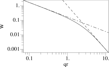
Figure 1: Dimensionless function $W$ vs. dimensionless distance $qr$. The two power-law asymptotes are shown (see details in the text).

To analyze the influence of the additional potential mediated by static magnetic dipole-dipole interactions, we average Eq. (10) over all angles and obtain in the ultracold-collision limit ($k\rightarrow 0$) the following equation:

$$\frac{1}{r^{2}}\frac{d}{dr}\left(r^{2}\frac{d}{dr}\psi_{\alpha}\right)+\frac{9ql_{m}^{2}W(qr)}{8r^{3}}\psi_{\alpha}=0,$$ (13)

where the quantity

$$l_{m}=\mu_{0}mg^{2}F^{2}/(4\pi\hbar^{2})$$ (14)

is the characteristic magnetic length. Equation (13) must be supplemented by the hard-sphere boundary condition

$$\psi_{\alpha}(a)=0$$ (15)

that accounts for the short-range (van der Waals) interactions. Solution of Eqs. (13), (15) yields the modified scattering length $\tilde{a}$, which can be inferred from the $r\rightarrow\infty$ asymptotics of the solution that is propoportional to $1-\tilde{a}/r$.

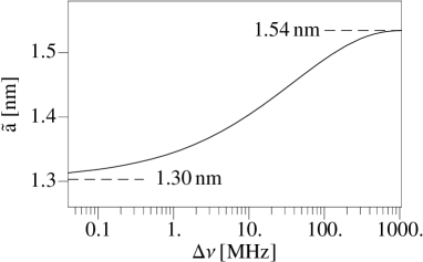
Figure 2: Modified scattering length for ⁵⁰Cr vs. frequency splitting $\Delta\nu=\Delta E/(2\pi\hbar)$. The two asymptotes of $\tilde{a}$ in the small- and large-$q$ limits are shown.

It is noteworthy that for $q\rightarrow 0$ the magnetically-induced isotropic potential varies as $r^{-4}$ and does not depend on $q$. In this case Eqs. (13), (15) admit an analytical solution,

$$\psi_{\alpha}(r)=\sin\left[\frac{\sqrt{3}l_{m}}{4a}\left(1-\frac{a}{r}\right)\right],$$ (16)

so that the modified scattering length becomes

$$\tilde{a}|_{q\rightarrow 0}=a\frac{\sqrt{3}l_{m}/(4a)}{\tan[\sqrt{3}l_{m}/(4a)]}.$$ (17)

In Fig. 2 we plot the results of numerical integration of Eq. (13) for ⁵⁰Cr. This isotope is chosen because chromium atoms have quite a large magnetic moment, $gF=6\mu_{B}$, $\mu_{B}$ being the Bohr magneton. On the other hand, the bare (unaffected by the effect under consideration) scattering length $a$ for this isotope in the state of the maximum spin projection is of about 29 Bohr’s radii, as can be concluded by mass-scaling arguments from the most recent data on ⁵²Cr scattering crscat . Note, that the recent, more accurate measurements cranew yield smaller values of the scattering length for ⁵²Cr and, consequently, for ⁵⁰Cr, than the previously reported data craold . The value $a=1.54$ nm is smaller than $l_{m}=2.34$ nm, and the difference between $a$ and $\tilde{a}$ becomes observable (up to 15 %). By contrast, the scattering length for ⁵²Cr is three times larger than for ⁵⁰Cr. As a result, the influence of static magnetic dipole interactions in the case of ⁵²Cr is negligible.

The discussed mechanism of the scattering length modification will manifest itself via excitation of BEC oscillations by periodic modulation of the external uniform magnetic field. Such a method to reveal the scattering length modulation has been proposed with regard to Feshbach resonance kagan . Consider a BEC of ⁵⁰Cr in the Thomas-Fermi regime pethick trapped in an optical dipole harmonic potential, which is assumed, for the sake of simplicity, to be isotropic, $\omega_{0}$ being its fundamental frequency. The uniform, $z$-directed magnetic field oscillates in time as

$$B(t)=B_{0}+B_{1}\sin\omega t.$$ (18)

Its variation results in variation of the frequency splitting $\Delta\nu$ between the states $|\alpha\rangle$ and $|\beta\rangle$. The Zeeman shift in a weak field is given by $\Delta\nu/B=87.7$ MHz/mT. Thus we can infer the time variation of the scattering length using the dependence $\tilde{a}(\Delta\nu)$ plotted in Fig. 2.

Let the magnetic field oscillations be switched on at $t=0$. The lowest monopole (angle-independent) mode of the BEC oscillations is described by the nonlinear equation kagan

$$\ddot{b}+\omega_{0}^{2}b=\tilde{a}(t)/(\tilde{a}_{0}b^{4}),$$ (19)

where $b=R/R_{0}$ is the ratio of the Thomas-Fermi radius $R$ of the oscillating BEC to the BEC radius at rest, $R_{0}=R|_{t=0}=l_{ho}(N\tilde{a}_{0}/l_{ho})^{1/5}$ pethick , $\tilde{a}_{0}=\tilde{a}|_{t=0}$, $l_{ho}=\sqrt{\hbar/(m\omega_{0})}$, $N$ is the number of atoms in the BEC. For the numerical estimations we take $\omega_{0}/(2\pi)\sim 100$ Hz, $N\sim 10^{5}$, thus obtaining $R_{0}\sim 6~{}\mu$m and the peak density of the BEC of about $3\cdot 10^{14}$ cm^-3. The initial conditions to Eq. (19) are $b|_{t=0}=1$, $\dot{b}|_{t=0}=0$.

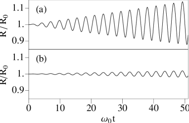
Figure 3: Relative (dimensionless) modulation of the Thomas-Fermi BEC radius vs. dimensionless time under the action of the variable magnetic field Eq. (18). (a) $B_{0}=0.08$ mT, (b) $B_{0}=0.6$ mT; $B_{1}=0.04$ mT in both the cases.

Choosing the frequency of the magnetic field modulation $\omega=\sqrt{5}\omega_{0}$, we ensure the resonance of the parametric excitation with the lowest monopole mode in the linear regime. In Fig. 3 we present the numerical solution of Eq. (19) for two different choices of the magnetic field parameters. While the amplitude $B_{1}$ of the magnetic field oscillations is the same, the mean value, $B_{0}$, takes two distinct values. In Fig. 3(a) $B_{0}$ corresponds to the steepest derivative $d\tilde{a}/dB$, so that the BEC excitations are excited most efficiently. For our numerical estimations we take $\omega_{0}/(2\pi)\sim 100$ Hz, $N\sim 10^{5}$, thereby obtaining the Thomas-Fermi BEC radius $R_{0}\sim 6~{}\mu$m and the peak density of the BEC of about $3\cdot 10^{14}$ cm^-3. Thus for the parameters of Fig. 3(a), after 80 ms the amplitude of oscillations of the Thomas-Fermi BEC radius approaches $0.84~{}\mu$m. This amplitude is approximately twice larger than the resonant wavelength of the optical ${}^{7}S_{3}\leftrightarrow^{7}P_{3}$ transition in chromium, thus making the BEC oscillations detectable by optical imaging. By contrast, the value of $B_{0}$ in Fig. 3(b) corresponds to a relatively small $d\tilde{a}/dB$ and, therefore, to much less efficient excitation of the BEC.

To conclude, we have proposed a new mechanism of $s$-wave scattering length tuning and modulation, different from both Feshbach-resonance feshbach and confinement-induced resonance methods cir1d ; cir2d . It involves a hitherto unexplored aspect of ultracold-atom collisions, namely, their nonlocality mediated by fluctuations of the magnetic dipole moments. Magnetic dipole-dipole interaction causes virtual transitions between different Zeeman sublevels of the atomic ground state. Such a coupling to the virtual state induces, additionally to van der Waals forces, an attractive isotropic interatomic potential. If the energy gap $\Delta E$ between the occupied and virtual spin states grows to infinity, we recover the “bare” (unmodified) scattering length value $a$, which is calculated from the van der Waals (non-magnetic) potential only. As $\Delta E$ vanishes, the renormalized scattering length approaches the limit (17) that is fully determined by the ratio of the magnetic length $l_{m}$, Eq. (14), to $a$. An appreciable effect is expected for $l_{m}/a\gtrsim 1$, which is the case for ⁵⁰Cr atoms, where we expect lowering of the modified scattering length by up to 15 % with respect to $a$.

This work is partially supported by the German-Israeli Foundation, the EC (SCALA NOE), and ISF. I.E.M. also acknowledges support from the program Russian Leading Scientific Schools (grant 9879.2006.2). The authors thank Prof. T. Pfau for helpful discussions.

References

- (1) F. Dalfovo, S. Giorgini, L.P. Pitaevskii, and S. Stringari, Rev. Mod. Phys. 71, 463 (1999); A.J. Leggett, Rev. Mod. Phys. 73, 307 (2001).
- (2) E. Tiesinga, B.J. Verhaar, H.T.C. Stoof, Phys. Rev. A 47, 4114 (1993); Ph. Courteille, R.S. Freeland, D.J. Heinzen, F.A. van Abeelen, and B.J. Verhaar, Phys. Rev. Lett. 81, 69 (1998); J.L. Roberts, N.R. Claussen, J.P. Burke, Jr., C.H. Greene, E.A. Cornell, and C.E. Wieman, Phys. Rev. Lett. 81, 5109 (1998); J. Stenger, S. Inouye, M.R. Andrews, H.-J. Miesner, D.M. Stamper-Kurn, and W. Ketterle, Phys. Rev. Lett. 82, 2422 (1999).
- (3) M. Olshanii, Phys. Rev. Lett. 81, 938 (1998); H. Moritz, T. Stöferle, K. Günter, M. Köhl, and T. Esslinger, Phys. Rev. Lett. 94, 210401 (2005).
- (4) D.S. Petrov, M. Holzmann, and G.V. Shlyapnikov, Phys. Rev. Lett. 84, 2551 (2000).
- (5) L. Santos, G.V. Shlyapnikov, P. Zoller, and M. Lewenstein, Phys. Rev. Lett. 85, 1791 (2000); K. Góral, K. Rza̧żewski, and T. Pfau, Phys. Rev. A 61, 051601(R) (2000) K. Góral and L. Santos, Phys. Rev. A 66, 023613 (2002); S. Giovanazzi, A. Görlitz, and T. Pfau, Phys. Rev. Lett. 89, 130401 (2002); D.H.J. O Dell, S. Giovanazzi, and C. Eberlein, Phys. Rev. Lett. 92, 250401 (2004)
- (6) J. Stuhler, A. Griesmaier, T. Koch, M. Fattori, T. Pfau, S. Giovanazzi, P. Pedri, and L. Santos, Phys. Rev. Lett. 95, 150406 (2005).
- (7) D. O’Dell, S. Giovanazzi, G. Kurizki, and V.M. Akulin, Phys. Rev. Lett. 84, 5687 (2000). S. Giovanazzi, D. O’Dell, and G. Kurizki, Phys. Rev. Lett. 88, 130402 (2002); D.H.J. O Dell, S. Giovanazzi, and G. Kurizki, Phys. Rev. Lett. 90, 110402 (2003).
- (8) M. Marinescu and L. You Phys. Rev. Lett. 81, 4596 (1998); S. Yi and L. You, Phys. Rev. A 61, 041604(R) (2000).
- (9) D.C.E. Bortolotti, S. Ronen, J.L. Bohn, and D. Blume, Phys. Rev. Lett. 97, 160402 (2006); S. Ronen, D.C.E. Bortolotti, D. Blume, and J.L. Bohn, Phys. Rev. A 74, 033611 (2006).
- (10) J.J. Sakurai, Modern Quantum Mechanics, (Addison-Wesley, Reading, Mass., 1994), p. 382.
- (11) H. Nakamura, J. Phys. Soc. Japan 35, 848 (1973).
- (12) D.A. Varshalovich, A.N. Moskalev, and V.K. Khersonsky, Quantum Theory of Angular Momentum (World Scientific, Singapore, 1988), p. 165.
- (13) T. Pfau, private communication (2006).
- (14) J. Werner, A. Griesmaier, S. Hensler, J. Stuhler, T. Pfau, A. Simoni, and E. Tiesinga, Phys. Rev. Lett. 94, 183201 (2005); A. Griesmaier, J. Stuhler, T. Koch, M. Fattori, T. Pfau, and S. Giovanazzi, arXiv: cond-mat/0608171.
- (15) P.O. Schmidt, S. Hensler, J. Werner, A. Griesmaier, A. Görlitz, T. Pfau, and A. Simoni, Phys. Rev. Lett. 91, 193201 (2003).
- (16) Yu. Kagan, E.L. Surkov, and G.V. Shlyapnikov, Phys. Rev. Lett. 79, 2604 (1997).
- (17) G. Baym and C.J. Pethick, Phys. Rev. Lett. 76, 6 (1996).
- (18) S. Stringari, Phys. Rev. Lett. 77, 2360 (1996).