Athermal Shear-Transformation-Zone Theory of Amorphous Plastic Deformation II: Analysis of Simulated Amorphous Silicon

Abstract

In the preceding paper, we developed an athermal shear-transformation-zone (STZ) theory of amorphous plasticity. Here we use this theory in an analysis of numerical simulations of plasticity in amorphous silicon by Demkowicz and Argon (DA). In addition to bulk mechanical properties, those authors observed internal features of their deforming system that challenge our theory in important ways. We propose a quasithermodynamic interpretation of their observations in which the effective disorder temperature, generated by mechanical deformation well below the glass temperature, governs the behavior of other state variables that fall in and out of equilibrium with it. Our analysis points to a limitation of either the step-strain procedure used by DA in their simulations, or the STZ theory in its ability to describe rapid transients in stress-strain curves, or perhaps to both. Once we allow for this limitation, we are able to bring our theoretical predictions into accurate agreement with the simulations.

I Introduction

In the preceding paper BLP06 , we presented an athermal STZ theory of plastic deformation in materials where thermal activation of irreversible molecular rearrangements is negligible or nonexistent. Here we use that theory to interpret an extensive body of computational data published recently by Demkowicz and Argon 04DA ; DA1 ; DA2 ; 06AD , hereafter referred to occasionally as “DA.” Those authors simulated plastic deformation in amorphous silicon using a system of 4096 atoms interacting via a Stillinger-Weber potential 85SW in a cubic cell with periodic boundary conditions. They subjected this system to pure shear under both constant-volume and constant-zero-pressure, plane-strain, conditions. Their reports of these simulations are remarkably complete and detailed. They provide valuable and challenging information about:

• the relation between stress-strain response and sample preparation;

• the theoretical description of nonequilibrium behavior in systems subject to steady-state and transient mechanical deformation;

• the nature of the glass transition in simulated amorphous silicon;

• the strengths and limitations of numerical simulation techniques.

We address each of these topics in the body of this report.

Demkowicz and Argon used two different procedures for simulating shear deformation. In their potential energy minimization method (PEM), each step in the process consisted of a small, affine, shear displacement of all the atomic positions, followed by a minimization of the potential energy during which the atoms relax to their nearby positions of mechanical equilibrium. Supposedly, PEM simulations correspond to the limit of zero strain rate at zero temperature, but that interpretation is problematic. In their molecular dynamics (MD) method, DA used a different step-strain procedure in which each small shear increment was followed by an MD relaxation at temperature $T=300\,K$, with an average strain rate of order $10^{8}\,{\rm sec}^{-1}$. In both procedures, an incremental shear was imposed only after the system was judged to have reached a stable, stationary state following the preceding step. We argue below that there are important uncertainties associated with both of these step-strain simulation methods.

The single most important feature of the DA simulations is that, in addition to measuring the shear stress (and keeping track of pressure and/or volume changes) during deformation, DA also observed local atomic correlations within their system. Here they were taking advantage of their numerical method to see inside their system in a way that is seldom possible in laboratory experiments using real materials. They found that the environments of some atoms were solidlike and others liquidlike, and that the liquidlike regions seemed to be, as they say, the “plasticity carriers.” Before any mechanical deformation, their fraction of liquidlike regions $\phi$ was small when the system was annealed or cooled slowly, and was approximately 0.5 when the system was quenched rapidly. Then, during constant-zero-pressure deformations, $\phi$ approached a value slightly less than 0.5, independent of its initial value. Thus, $\phi$ behaved in a manner qualitatively similar to the dimensionless effective temperature $\chi$ or, equivalently, the density of STZ’s $\Lambda\propto\exp(-1/\chi)$ described in BLP06 . The relation between these quantities is one of the main topics to be addressed in this paper.

Amorphous silicon, like water, expands as it solidifies. Moreover, its properties are highly sensitive to small changes in density. A slowly quenched, more nearly equilibrated system is less dense than one that is rapidly quenched, because the former contains a smaller population of denser, liquidlike regions than the latter. When strained, the more nearly equilibrated system initially responds elastically, and takes longer than a rapidly quenched system to generate enough plasticity carriers to enable plastic flow. Accordingly, the equilibrated system exhibits a more pronounced stress peak of the kind illustrated in Figure 1 (top curve, upper panel) of BLP06 . As the liquidlike fraction $\phi$ increases, the system contracts if held at constant pressure; or else, if the system is held at constant volume, the pressure decreases and may even become negative. It may be surprising to theorists but nevertheless is true that, in this material, the STZ’s must be associated with decreases rather than increases in free volume.

For theoretical purposes, it will be simplest to look only at constant-pressure simulations, because the changes in pressure that occur at constant volume require additional, hard-to-control approximations for behaviors that are not intrinsic to the STZ hypotheses. System-specific parameters such as the yield stress $s_{y}$ are likely to be more sensitive to changes in pressure than in volume. For example, the Mohr-Coulomb effect implies that $s_{y}$ increases with pressure. Demkowicz and Argon point out that direct evidence for pressure dependence can be seen in the graphs of the liquid fraction $\phi$ as a function of strain $\gamma$ in Figs. 10(c) and 15(c) of DA1 . In the constant-zero-pressure simulations shown in their Fig. 15, $\phi$ equilibrates to approximately the same value after deformation for all four different initial conditions. That does not happen in the constant-volume simulations in Fig. 10, implying that the internal states of these deformed systems differ from one another in nontrivial ways.

In addition to the questions pertaining to step-strain procedures, to be discussed in detail in Sec. IV, there are other limitations of the DA simulations that must be taken into account. The DA simulation system is too small to make it likely that more than one STZ-triggered event is taking place within a characteristic plastic relaxation time; and data is reported only for single numerical experiments performed on individual samples rather than averages over multiple experiments. Thus, fluctuations are large, and the results must be sensitive to statistical variations in initial conditions. In short, we must be careful in our interpretations.

On the positive side, Demkowicz and Argon’s remarkable combination of multiple simulation methods and multiple observations allows us to use the athermal STZ theory to construct what we believe is an internally self-consistent interpretation of their data. Going beyond their stress-strain curves, and focusing on the behaviors of the liquidlike fraction $\phi$ and the density $\rho$, we develop a quasithermodynamic picture in which the effective disorder temperature $\chi$ plays a dominant role. In this picture, the STZ’s, i.e. the active flow defects, are rare sites, out in the wings of the disorder distribution, that are more susceptible than their neighbors to stress-induced shear transformations. They almost certainly lie in the liquidlike regions of the system, but only a very small fraction of the liquidlike sites are STZ’s. The energy dissipated in the STZ-initiated transitions generates the effective temperature $\chi$, a systemwide intensive quantity that, in turn, determines extensive quantities such as $\phi$ and $\rho$.

Our central hypothesis is that there exist quasithermodynamic equations of state relating steady-state values of $\phi$ and $\rho$ to $\chi$ (and also, in principle, to the pressure and shear stress). Once we have found these equations of state, we extend the quasithermodynamic model to describe the way in which $\phi$ and $\rho$ fall in and out of equilibrium with $\chi$ during transient responses to external driving forces. In this way, we arrive at a quantitative interpretation of the DA simulations.

We begin in Sec. II with a brief summary of the athermal STZ theory developed in BLP06 . Section III contains a preliminary analysis of the DA stress-strain data. In Sec. IV, we explain why we cannot accept the initially good agreement between the STZ theory and the simulation data. These arguments motivate the quasithermodynamic hypothesis, introduced in Sec. V. We extend the quasithermodynamic ideas to nonequilibrium situations in Sec. VI. Finally, in Sec. VII, we conclude with some speculations concerning the validity of the quasithermodynamic picture and its relation to the STZ theory in general.

II STZ Summary

In order to make this paper reasonably self-contained, we start by restating Eqs. (3.12) - (3.16) in BLP06 . The first of these equations is an expression for the total rate of deformation tensor $D^{tot}=\dot{\gamma}/2$ as the sum of elastic and plastic parts:

$$D^{tot}={\dot{\tilde{s}}\over 2\,\tilde{\mu}}+D^{pl}(\tilde{s},m,\Lambda),$$ (1)

where $\tilde{s}$ and $\tilde{\mu}$ are the deviatoric stress and the shear modulus measured in units of the yield stress $s_{y}$. The internal state variables $m$ and $\Lambda$ are, respectively, the orientational bias and the scaled density of STZ’s. We consider only the case of pure, plane-strain shear in which the material is strained at a fixed rate $\dot{\gamma}$, and the stress is measured as a function of the strain $\gamma$. To describe such experiments, we write Eq.(1) in the form

$${d\tilde{s}\over d\gamma}=\tilde{\mu}\,\left(1-{2\,\epsilon_{0}\,\Lambda\over\dot{\gamma}\,\tau_{0}}\,q(\tilde{s},m)\right),$$ (2)

where $\epsilon_{0}$ is a number of order unity (the atomic density in atomic units multiplied by the incremental strain associated with an STZ transition), $\tau_{0}$ is the characteristic time scale for STZ transitions, and

$$q(\tilde{s},m)\equiv{\mathcal{C}}(\tilde{s})\,\Bigl{(}{\tilde{s}\over|\tilde{s}|}-m\Bigr{)}.$$ (3)

The function ${\cal C}(\tilde{s})$ describes the stress dependence of the STZ transition rate; it is proportional to $|\tilde{s}-1|$ for $|\tilde{s}|\gg 1$ and vanishes smoothly near $\tilde{s}=0$. As defined by Eq.(3.6) in BLP06 , the smoothness of ${\cal C}(\tilde{s})$ near $\tilde{s}=0$ is determined by a parameter $\zeta$, which we take to be unity throughout the following.

Similarly, we restate Eqs. (3.9), (3.10) and (3.11) from BLP06 :

$${dm\over d\gamma}={2\over\dot{\gamma}\,\tau_{0}}\,q(\tilde{s},m)\,\Bigl{(}1-{m\,\tilde{s}\over\Lambda}\,e^{-1/\chi}\Bigr{)};$$ (4)

$${d\Lambda\over d\gamma}={2\over\dot{\gamma}\,\tau_{0}}\,\tilde{s}\,q(\tilde{s},m)\,\bigl{(}e^{-1/\chi}-\Lambda\bigr{)};$$ (5)

and

$${d\chi\over d\gamma}={2\,\epsilon_{0}\over c_{0}\,\dot{\gamma}\,\tau_{0}}\,\Lambda\,\tilde{s}\,q(\tilde{s},m)\,(\chi_{\infty}-\chi).$$ (6)

The constant $c_{0}$ is a configurational specific heat per atom in units $k_{B}$, which must be of order unity.

We assume that the stress and strain tensors in these equations remain diagonal in two dimensional pure shear and plane strain, and that any correction in the third dimension is negligible in comparison to other uncertainties in this analysis. A basic premise of the STZ theory is that the zones are rare and do not interact with each other; thus we assume from the beginning that the quantity $\epsilon_{0}\,\exp(-1/\chi)$ is small of order $10^{-3}$ (in fact, very much less), so that the equations for $m(\gamma)$ and $\Lambda(\gamma)$ are stiff compared to those for $\tilde{s}(\gamma)$ and $\chi(\gamma)$. Then we can safely replace Eqs. (4) and (5) by their stationary solutions:

$$m=m_{0}(\tilde{s})=\cases{\tilde{s}/|\tilde{s}|&if $|\tilde{s}|\leq 1$\cr 1/\tilde{s}&if $|\tilde{s}|>1$}$$ (7)

and

$$\Lambda=e^{-1/\chi}.$$ (8)

Eqs. (2) and (6) become:

$${d\tilde{s}\over d\gamma}=\tilde{\mu}\,\left(1-{2\,\epsilon_{0}\,\over q_{0}}\,e^{-1/\chi}\,q(\tilde{s})\right),$$ (9)

and

$${d\chi\over d\gamma}={2\,\epsilon_{0}\over c_{0}\,q_{0}}\,e^{-1/\chi}\,\tilde{s}\,q(\tilde{s})\,(\chi_{\infty}-\chi),$$ (10)

where

$$q(\tilde{s})={\mathcal{C}}(\tilde{s})\,\Bigl{(}{\tilde{s}\over|\tilde{s}|}-m_{0}(\tilde{s})\Bigr{)},$$ (11)

and $q_{0}=\dot{\gamma}\,\tau_{0}$.

III First Fits to the DA Stress-Strain Curves

The first step in our STZ analysis of the DA data is to use Eqs. (9) - (11) to fit the stress-strain curves in Fig. 15(a) of DA1 , shown here in Fig. 1. These two equations involve the parameters $q_{0}$ (the dimensionless strain rate), $s_{y}$ (needed in order to convert from dimensionless stresses $\tilde{s}$ to measured stresses in units GPa), $\tilde{\mu}$, $c_{0}$, $\chi_{\infty}$, and the four initial values of the effective temperature $\chi(0)=\chi_{0}$.

We can obtain a certain amount of information about these parameters directly from features of the stress-strain curves before doing any computation. Note from Eqs. (7) and (11) that no plastic deformation occurs for $\tilde{s}<1$, no matter how large $\chi$ might be. Thus the lowest observed value of a stress that marks a departure from elastic behavior is an upper bound for $s_{y}$. The bottom stress-strain curve in Fig. 1, which is the curve with the largest initial value of $\phi$, seems to have a break point that is about a factor of three less than the flow stress $s_{f}$, which we see from the figure is about 1.06 GPa. Therefore, $s_{y}\cong s_{f}/3\cong 0.35$ GPa, and $\tilde{s}_{f}\cong 3$. We take the shear modulus $\mu\cong 46$ GPa directly from the slope of the stress-strain curves in the elastic region; thus we choose $\tilde{\mu}\cong 130$. Setting the right-hand side of Eq.(9) to zero, we find that the flow stress $\tilde{s}_{f}$ satisfies

$$q_{0}=\dot{\gamma}\,\tau_{0}=2\,\epsilon_{0}\,e^{-1/\chi_{\infty}}\,q(\tilde{s}_{f}).$$ (12)

Using this relation with the DA estimate of $\dot{\gamma}$ and the value of $\chi_{\infty}$ given below, we confirm that $\tau_{0}$ is of order femtoseconds as implied by the Stillinger-Weber interactions used in these simulations.

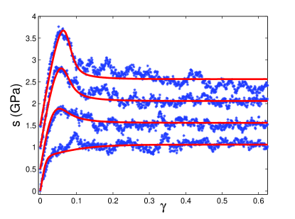
Figure 1: Theoretical stress-strain curves (solid lines) compared to the DA numerical simulation data DA1 . The parameters used are: $\epsilon_{0}=1$, $s_{f}=1.06$GPa, $\mu=46$ GPa, $s_{y}=0.35$ GPa, $c_{0}=0.18$ and $\chi_{\infty}=0.065$. The initial effective temperatures are: $\chi_{0}$= $0.0559,\,0.0580,\,0.0612,\,0.0680$ (from top to bottom). The curves are shifted by 0.5 GPa for clarity.

Once we have inserted Eq. (12) into Eqs. (9) and (10), we can solve these equations and vary the remaining parameters to fit the stress-strain curves in Fig. 15 (a) of DA1 . We find that the fits are disappointingly insensitive to our choice of $\epsilon_{0}\,\exp(-1/\chi_{\infty})$ so long as we stay within our constraint that this product be small. However, our later analysis of the liquidlike fraction $\phi$ reveals that the internally consistent value of $\chi_{\infty}$ is $0.065$, which is slightly bigger than our a priori order-of-magnitude estimate based on the experimental data, as shown in JOHNSON for example, but seems well within the accuracy of our approximation for $\chi_{\infty}$ in 04Lan and the uncertainties of these small-scale simulations. Therefore we have chosen $\epsilon_{0}=1$ and $\chi_{\infty}=0.065$. Agreement between theory and the numerical simulations then can be obtained for all four of the stress-strain curves by setting $c_{0}=0.18$ and adjusting only $\chi_{0}$ for each curve. Our best-fit results are shown in Fig. 1. The corresponding values of $\chi_{0}$ (from top to bottom in the figure) are $0.0559,\,0.0580,\,0.0612,\,0.0680$. Note that there is a gap in $\chi_{0}$ between the lowest three values, for which the stress-strain curves are peaked, and the largest, which shows no peak.

If it were useful to do so, we could improve the agreement between the simulated stress-strain curves and our theory by making small adjustments of $s_{y}$ and $\tilde{\mu}$ for each curve, consistent with the likelihood that the four relatively small computational systems are not exactly comparable to each other in their as-quenched states. In the spirit of the discussion to follow, however, we have chosen to assume that the four systems reach effectively identical steady states after persistent shear deformation, and to attribute the small discrepancies to the statistical uncertainties visible in the data. The only systematic feature of the stress-strain data that is not recovered by the theory is the slow decrease of the flow stress with increasing strain in the top curve (the one with the most pronounced stress peak). We believe that this behavior is caused by the emergence of a nascent shear band as illustrated in Fig. 16(b) of DA1 .

IV Second Thoughts

Fitting the stress-strain curves, however, is only a part of the challenge of interpreting the DA data DA1 . We also must understand how the liquidlike fraction $\phi$ and the density $\rho$ relate to our STZ variables, especially the effective temperature $\chi$. Therefore, it is essential to know whether we can trust the values of $\chi_{0}$ deduced from the STZ analysis of the stress-strain curves. We argue in the following paragraphs that these values are not quantitatively reliable.

One of the key tenets of plasticity theory is that transient peaks observed in the stress-strain curves for well annealed samples occur because there is an initial lack of plasticity carriers in these systems, and new carriers must be generated by deformation before plastic flow can begin and the stress can relax. Demkowicz and Argon use the correlation between stress peaks and the liquidlike fraction $\phi$ to argue that $\phi$ is a direct measure of the population of plasticity carriers. The STZ theory, as presently constituted, predicts stress peaks when – and only when – the initial STZ density is small.

This tenet is not confirmed by the DA simulations. Note first the data for $\phi$ as a function of strain $\gamma$ shown by DA in Fig.15 of DA1 , also shown here in Fig.6. There are four curves. Two of them have small initial values of $\phi(\gamma=0)=\phi_{0}$ and exhibit stress peaks. The corresponding values of $\phi(\gamma)$ rise monotonically to the steady-state value $\phi_{\infty}\cong 0.46$ as expected. Another curve starts with $\phi_{0}>\phi_{\infty}$. The corresponding stress-strain curve has no peak, and $\phi(\gamma)$ decreases to $\phi_{\infty}$, again in accord with expectations. In one case (the one with $\phi_{0}\cong 0.46$), however, $\phi_{0}$ is slightly above $\phi_{\infty}$ but the stress still shows a peak. Moreover, the corresponding density $\rho$ decreases with $\gamma$, implying that the denser liquidlike fraction is decreasing during the deformation.

This kind of behavior appears elsewhere in the DA papers 04DA ; DA1 ; DA2 ; 06AD . It is clear in the constant-volume, MD simulations, where one of the stress-strain curves has a peak, but the corresponding $\phi(\gamma)$ remains nearly constant, and the pressure increases instead of decreasing as it should if the liquidlike fraction were growing. And, as we note below, all of the PEM simulations in DA2 show stress peaks, even the ones in which $\phi_{0}$ is large and comparable to $\phi_{\infty}$.

It seems to us that the most likely explanation for these discrepancies is that the ubiquitous stress peaks are artifacts of the step-strain simulations. It is also quite possible, of course, that the STZ theory does not adequately account for the way in which stresses respond to rapid changes in the strain rate, and that the DA simulations are simply out of range of our STZ analysis. Perhaps both explanations are in part correct. Nevertheless, we prefer the first explanation for the following reasons.

Demkowicz and Argon performed only MD simulations, and not PEM, at constant-pressure; but a number of features of their PEM results may be relevant here. They report that cascades of events were evident in their PEM simulations but were hard to detect in MD. Maloney and Lemaitre ML04a ; ML04b , who used only PEM, found that cascades were prevalent and sometimes so large that they spanned their systems, which were only two dimensional but larger in numbers of atoms than those used by DA. A related feature of the DA PEM simulations is that, even for rapidly quenched samples with large initial disorder, the stress-strain curves exhibit marked stress peaks followed by strain softening. We suspect that these behaviors may be generally characteristic of step-strain processes, and correspondingly uncharacteristic of continuous strain mechanisms that are more common in the laboratory.

Note that, between each strain increment in PEM, the system has a probability of dropping into a low energy state from which it cannot escape without the application of a large force. The large energy released when such a trapped state is destabilized may trigger cascades of smaller events. This trapping mechanism may be especially important at the beginning of a shear deformation, because then the energy minimization starts with a disordered, as-quenched system. As a result, the first energy drops may be large, and the initial stresses required to set the system into motion may be anomalously high. Thus we expect transient stress peaks in PEM, even for initially disordered systems; and we expect large stress fluctuations even in steady-state conditions. That is exactly what is seen by Demkowicz and Argon.

The difference between step strains and continuous shear has been demonstrated recently in bubble raft experiments by Twardos and Dennin DENNIN05 . Like Demkowicz and Argon, these authors subjected their strictly athermal system to both steady, slow shear and to discrete shear steps followed by relaxation periods long enough for most motion to cease. They monitored the stress during both procedures, with particular interest in the distribution of stress drops associated with irreversible plastic rearrangements. One of their most interesting results is that the average size of stress events decreases with decreasing shear rate for continuous strain, but increases for step strains. That is, the stress relaxes via a larger number of smaller drops for continuous deformation than for step-strain motion. Their interpretation of this result seems to us to be roughly consistent with our discussion of PEM simulations in the preceding paragraph; but neither they nor we claim a full understanding of this phenomenon

In their MD simulations, Demkowicz and Argon use step strains as opposed to a continuous strain rate. Apparently, allowing the system to relax for a time at $T=300\,K$ between strain steps removes the effects of at least some of whatever structural irregularities are producing cascades and stress peaks in the PEM simulations. It seems likely, however, that some elements of the athermal PEM-like, step-strain behavior persist in the MD results. Our hypothetical low-energy trapping states may be less likely to be sampled in step-strain MD, in which case the initial transients and steady-state stress fluctuations might be smoother, as indeed they are. But the step-strain MD procedure is not the same as a continuous one in which the strain is incremented on the time scale at which the molecular motions are resolved. In the DA simulations, the strain is incremented only once in about ten or more atomic vibration periods. We see little reason to believe that these two simulation procedures will produce precisely the same responses to rapidly changing driving conditions.

This situation forces us to conclude – reluctantly in view of the quality of the apparent agreement between the simulations and STZ theory shown in Fig. 1 – that the values of the $\chi_{0}$’s stated above and in the caption to Fig. 1 cannot be trusted.

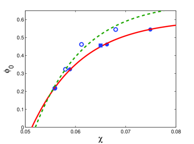
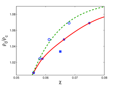
Figure 2: Upper panel: The equation of state $\phi=\phi_{0}(\chi)$ obtained by fitting the four data points (filled circles) plus $\phi_{\infty}=\phi_{0}(\chi_{\infty})=0.458$ (filled square). The $\phi_{0}$’s are the DA numerical simulation data DA1 ; the adjusted $\chi_{0}$’s are $0.0559,\,0.0589,\,0.0663$, and $0.0749$, with $\chi_{\infty}=0.065$. The solid line is our fit to these points in Eq. (13). The open circles are the observed $\phi_{0}$’s plotted against the unadjusted, best-fit, $\chi_{0}$’s. The dashed line is intended only as a guide for the eye. Lower panel: The equation of state $\rho=\rho_{0}(\chi)$ obtained by a procedure similar to the one described above except that the point $\rho_{\infty}=1.0335$ (filled square) is not included in the fit. We attribute its displacement from the equation of state to a stress-induced dilation. The density is normalized by $\rho_{c}$, the density of crystalline silicon (diamond cubic). The solid line is our smooth fit to the data. Again, the open circles and and dashed line indicate the unadjusted equation of state.

V Quasithermodynamic Hypotheses

Our inability to deduce the $\chi_{0}$’s from the stress-strain data has led us to probe more deeply into the meaning of the effective temperature in glass dynamics. We base our analysis on a set of quasithermodynamic hypotheses in which we assume that the steady-state properties of the configurational degrees of freedom below the glass transition are determined by the effective temperature $T_{eff}=(E_{STZ}/k_{B})\,\chi$, in close analogy to the way in which they are determined by the bath temperature $T$ above that transition. In true thermodynamic equilibrium, extensive quantities such as the density $\rho$, the internal energy $U$, or the liquidlike fraction $\phi$ in the DA simulations are functions of $T$ and the pressure $P$. In other words, these quantities obey equations of state. Below the glass transition, the configurational degrees of freedom – that is, the positions of the atoms in their inherent states – fall out of equilibrium with $T$ because thermally activated rearrangements are exceedingly slow or impossible. The most probable configurations in such situations maximize an entropy, thus the statistical distribution of these configurations is Gibbsian with $T=T_{eff}$.

Accordingly, our first hypothesis is that the high-$T$ equilibrium equations of state are preserved in the glassy state as expressions for the configurational parts of the extensive quantities $\rho$, $U$, $\phi$, etc. in terms of the intensive quantities $T_{eff}$, $P$, and the shear stress $s$. In particular, we propose that the effective temperatures $\chi_{0}$, multiplied by $E_{STZ}/k_{B}$, are the bath temperatures $T_{0}$ at which the DA simulation samples fell out of thermal equilibrium during cooling, and that the configurational parts of $\rho$, $U$, $\phi$, etc. were fixed at those temperatures. Our specialization to configurational parts recognizes that, for example, $\rho$ undergoes ordinary thermal expansion at small $T$ and that the total internal energy $U$ includes the kinetic energy. Both of those non-configurational parts are uninteresting for present purposes. Since we consider only $P=0$ situations and work only at fixed $T$, we omit explicit dependences on those variables. Shear dilation may be relevant, especially for determining $\rho$; but so long as we are considering only pre-deformation properties with $s=0$, we also omit explicit $s$ dependence. We return later to the question of shear dilation, and we also postpone a discussion of the potential energy. For the moment, we write simply: $\phi=\phi_{0}(\chi)$, $\rho=\rho_{0}(\chi)$.

As a first test of this hypothesis, we show by the open circles and dashed lines in both panels of Fig. 2 the functions $\phi_{0}(\chi)$ and $\rho_{0}(\chi)$ obtained with the measured values of $\phi_{0}$ and $\rho_{0}$ and our best-fit values of $\chi_{0}$ from Fig. 1. We do, in fact, find qualitatively plausible behavior. With our uncertainties about the $\chi_{0}$’s, however, we are obliged to look harder and bring other considerations to bear on this analysis.

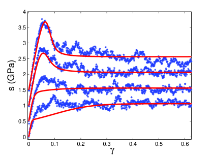
Figure 3: Modified stress-strain curves using $\chi_{0}=0.0559,\,0.0589,\,0.0663$, and $0.0749$. All other parameters are the same as those used in Fig. 1.

We know some qualitative features of these equations of state. First, we are dealing with a glass transition, and therefore we expect that $\phi_{0}(\chi)$ should extrapolate to some fixed value, possibly zero, at a nonzero Kauzmann temperature. In the following discussion, we define $\chi_{K}$ to be the effective temperature at which the extrapolated $\phi_{0}(\chi)$ vanishes; but we make no assumption about whether this is actually a Kauzmann temperature, or whether an ideal glass transition actually occurs at this or any other point.

Another feature is suggested by the binary, solidlike/liquidlike, nature of the atomic structure described by Demkowicz and Argon. If this were just a simple binary mixture, and if the energy of the mixture were proportional just to the density of the higher energy, liquidlike component, then the entropy would be a maximum at $\phi=1/2$ and the temperature would diverge at that point. Obviously, amorphous silicon is not so simple. Nevertheless, the observed $\phi$ does seem to have an upper bound not too far above $\phi=1/2$; thus, we expect that $\phi_{0}(\chi)$ saturates at some value $\phi_{0}=\phi_{{\rm lim}}\geq 0.55$ for large $\chi$.

Yet another consideration is that, in principle, we ought to be able to deduce the $T_{0}$’s directly from the graphs of density versus temperature for different quench rates shown in Fig. 1 of DA1 . The slowest quench is the closest to full equilibrium, and the points at which the faster quenches fall away from it are the three higher $T_{0}$’s. The lowest $T_{0}$ must be near the inflection point on the slow-quench curve. Unfortunately, the best we can do with the data at hand is estimate the $T_{0}$’s to about $\pm 20\,K$, and even then we must be cautious about systematic uncertainties in the simulations. Nevertheless, we can use this process as a rough check on the modifications of the $\chi_{0}$’s that we propose below.

We come now to our second and more speculative hypothesis – that the point $(\chi_{\infty},\,\phi_{\infty})$ ought to lie on the equilibrium equation-of-state curve; that is, $\phi_{\infty}=\phi_{0}(\chi_{\infty})$. Here we are assuming that persistent shear deformation in an athermal system rearranges the atomic configurations in a way that is statistically equivalent to thermally driven rearrangement, except that the relevant temperature is the effective disorder temperature $T_{eff}$ instead of the bath temperature $T$. We also are assuming that $\phi_{\infty}$, being a ratio of two populations, is insensitive to changes in the volume of the system that might occur during constant-zero-pressure simulations. In contrast, $\rho_{\infty}$ would decrease if, for example, the system undergoes a shear-induced dilation.

With these considerations in mind, our next step is to refine the estimates of the $T_{0}$’s by requiring that they produce smooth equations of state with the qualitative features hypothesized above, and that the observed $\phi_{\infty}\cong 0.458$ be equal to $\phi_{0}(\chi_{\infty})$. Accordingly, we have computed $\phi=\phi_{0}(\chi)$ and $\rho=\rho_{0}(\chi)$ by adjusting the $\chi_{0}$’s so as to optimize agreement with all the previously discussed constraints. Our results are shown by the solid lines in Fig. 2. As expected, $\rho_{\infty}<\rho_{0}(\chi_{\infty})$, because the flow stress $\tilde{s}_{f}$ at that point seems easily large enough to cause dilation. (Throughout this paper, values of $\rho$ are in units of $\rho_{c}=2323.8\,{\rm kg/m}^{3}$, the density of crystalline, diamond-cubic, silicon.) The effective Kauzmann temperature is $\chi_{K}=0.051$, and the upper bound for $\phi$ is $\phi_{{\rm lim}}=\phi(\chi\!\to\!\infty)\cong 0.6$. The smooth curve that we have fit to the equation of state for $\phi$, shown in the upper panel of Fig. 2, is

$$\phi_{0}(\chi)=\phi_{{\rm lim}}\,\left(1-e^{-a\,(\chi-\chi_{K})}\right),$$ (13)

where $a=100$. Other important parameters are the four $T_{0}$’s: $1100\,K,\,1160\,K,\,1305\,K,\,1475\,K$, which are consistent with our crude direct estimates from Fig. 1 in DA1 . Note that the large gap between the lowest three unadjusted $T_{0}$’s and the upper one has disappeared, and that the adjusted points fit on a smoother curve than the unadjusted ones. We also find that $T_{\infty}=1280\,K$. Then, with $\chi_{\infty}=0.065$, we obtain $E_{STZ}/k_{B}\cong 21,000\,K$, or about $1.3$ ev. The associated values of $\chi_{0}$ are $0.0559,\,0.0589,\,0.0663$, and $0.0749$.

Using these adjusted values of the $\chi_{0}$’s, we have recomputed and plotted the stress-strain curves in Fig. 3, shown again in comparison with the simulation data. As expected, the non-STZ peak has disappeared, and there is more rounding in the bottom, most rapidly quenched case, but the stress peaks for the two most deeply quenched systems remain almost unchanged.

Finally, within the context of quasithermodynamic equilibrium, we note that a relation between the potential energy and $\chi$ has been proposed and confirmed by Shi et al..SHI06 These authors describe molecular-dynamics simulations of shear banding in two-dimensional, non-crystalline, Lennard-Jones mixtures. Their analysis of these simulations goes beyond our own in at least one important way. They note that the plastic strain rate predicted by the STZ theory, as well as by other flow-defect theories, has the form $\exp(-1/\chi)$ multiplied by a function of the shear stress, essentially our factor $q(\tilde{s})$ defined in Eq.(11). Force balance requires that $\tilde{s}$ be a constant across the shear band, thus a measurement of the position-dependent strain rate is a measure of the position dependence of $\chi$. Shi et al. then postulate that the potential energy depends linearly on $\chi$. They compute the position-dependent potential energy directly from their simulation data and find that it maps accurately onto $\chi$ as predicted by the spatially varying strain rate. The importance of this observation is that they are looking at a weakly nonequilibrium situation in which the potential energy and $\chi$ are varying continuously in space, but only very slowly in time, along the postulated linear equation of state. Their system remains in quasithermodynamic equilibrium during this variation because, unlike the DA simulations discussed here, it is not undergoing a fast transient response to a sudden change in the applied stress. Thus their result anticipates and fits accurately into our quasithermodynamic picture.

VI Departures from Quasithermodynamic Equilibrium

The next question is whether the equilibrium equations of state shown in Fig. 2 are obeyed under nonequilibrium conditions during deformation. Apparently they are not. To see this, in Fig. 4, we have added to our equation-of-state graphs four data sets showing the observed values of $\phi$ and $\rho$ as functions of our calculated values of $\chi$ for the four different deformation histories. In all cases, the observed values of $\phi$ and $\rho$ initially fall off the equilibrium curves and do not come together again until they approach $\chi_{\infty}$. This nonequilibrium behavior can be seen more directly by comparing the three panels of Fig. 15 in DA1 . It is clear there that the rate at which the stress relaxes to the flow stress is faster than the rates at which either $\phi$ or $\rho$ relax to their steady-state values.

To account for the transient, nonequilibrium behavior of $\phi$, we propose an equation of motion analogous to Eq. (17) in 06AD , but with a form similar to our Eq. (10):

$${d\phi\over d\gamma}={2\,\epsilon_{0}\over c_{1}\,q_{0}}\,e^{-1/\chi}\,\tilde{s}\,q(\tilde{s})\,\left(\phi_{0}(\chi)-\phi\right),$$ (14)

where $c_{1}$ is a constant similar to $c_{0}$. The idea here is that the disorder described by $\chi$ may rise at its own rate, but the liquidlike-solidlike reorganization associated with $\phi$ may not catch up instantaneously. We assume that the underlying mechanism that determines these rates is still the rate of energy dissipation. There is no other comparably simple and basic coupling between mechanical deformation and the internal degrees of freedom that satisfies the requirement that it be a non-negative scalar. Note that Eq.(14) is supplementary to the STZ equations of motion, Eqs.(9) and (10); it assumes that the intensive quantities $\tilde{s}(\gamma)$ and $\chi(\gamma)$ are unchanged from the STZ predictions and that they continue to control the behavior of $\phi$ even away from equilibrium. This is a strong assumption, especially near the initial stress transients where we already know that there is some mismatch between the STZ theory and the DA simulations.

Our results for the four functions $\phi(\chi)$, determined using Eq.(14), are shown in Fig.5. The corresponding functions $\phi(\gamma)$ are shown in Fig.6, here in comparison with the DA data. The only adjustable parameter is $c_{1}$, which we choose to be $0.42$. The agreement seems to be within the uncertainties of the data.

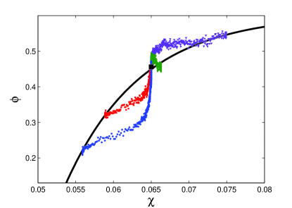
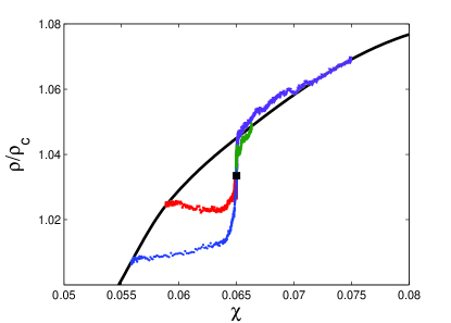
Figure 4: Upper panel: The DA numerical simulation data for $\phi$ versus the theoretical $\chi$ for the four cases considered in Ref. DA1 . The equation of state $\phi=\phi_{0}(\chi)$ was added to stress the nonequilibrium nature of the deformation-induced dynamics of $\phi$. Lower panel: The corresponding plot for $\rho/\rho_{c}$. The points $(\chi_{\infty},\,\phi_{\infty})$ and $(\chi_{\infty},\,\rho_{\infty})$ are marked by solid squares.

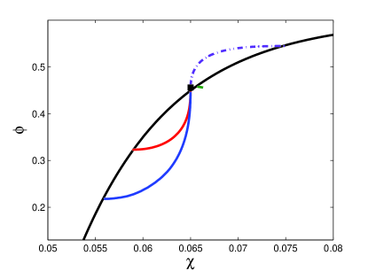
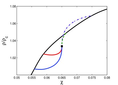
Figure 5: Upper panel:$\phi$ as a function of $\chi$ using the nonequilibrium Eq. (14) with $c_{1}=0.42$. The equilibrium equation of state was added for illustration. The curves should be compared to the DA data shown in the upper panel of Fig. 4. Lower panel: $\rho$ as a function of $\chi$ using the nonequilibrium Eq. (15) with $c_{1}=0.42$. These curves should be compared to the DA data shown in the lower panel of Fig. 4. The points $(\chi_{\infty},\,\phi_{\infty})$ and $(\chi_{\infty},\,\rho_{\infty})$ are marked by solid squares.

We continue our development of the nonequilibrium quasithermodynamic theory by writing an equation analogous to Eq. (14) for the function $\rho(\gamma)$:

$${d\rho\over d\gamma}={2\,\epsilon_{0}\over c_{1}\,q_{0}}\,e^{-1/\chi}\,\tilde{s}\,q(\tilde{s})\,\left(\rho_{0}(\chi)-\rho-\delta\rho_{0}\right),$$ (15)

Here, $\delta\rho_{0}\cong 0.012$ is the dilation-induced shift of the equilibrium density shown by the displacement of $\rho_{\infty}$ from the equilibrium curve $\rho_{0}(\chi)$ in the lower panel of Fig.2. To integrate Eq.(15), we have approximated $\rho_{0}(\chi)$ by a smooth polynomial. The factor $c_{1}=0.42$ needed to fit the density data is the same as in Eq. (14). The corresponding graphs of $\rho(\gamma)$, along with the DA data, are shown in Fig. 7. Again, the agreement seems to be within the uncertainties; but here we are pushing the theory too far for comfort. Our quasithermodynamic hypotheses imply that $\rho_{0}(\chi)$ ought to be a function of the shear stress $\tilde{s}$ as well as $\chi$, and that the dilation approximated here by $\delta\rho_{0}$ should be part of that generalized equation of state. In particular, $\delta\rho_{0}$ should be the dilational change in the density when $\tilde{s}$ is equal to the flow stress $\tilde{s}_{f}$. We have in fact tried $\delta\rho_{0}\propto\tilde{s}^{2}$ (as in nonlinear elasticity), but the results are distinctly unsatisfactory at small $\gamma$ where neither Eq.(15) nor the STZ theory itself may accurately describe the fast transient. Equations (14) and (15) do account for the relatively slow relaxation of $\phi(\gamma)$ and $\rho(\gamma)$ as compared to that of $\tilde{s}(\gamma)$. This level of success seems to be as much as we can expect from the theory at this stage in its development.

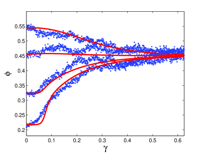
Figure 6: Theoretical predictions of $\phi(\gamma)$ for all four quenches, based on Eq. (14) with $c_{1}=0.42$, compared with the DA simulation data.

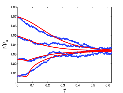
Figure 7: Theoretical predictions of $\rho(\gamma)$ for all four quenches, based on Eq. (15) with $c_{1}=0.42$, compared with the DA simulation data.

VII Summary and Concluding Remarks

The unique aspect of the Demkowicz and Argon simulations is their measurement of extensive quantities – the mass density $\rho$ and the liquidlike fraction $\phi$ – in parallel with conventional stress-strain curves. They argue convincingly and importantly that $\phi$ is closely related to the density of plasticity carriers. However, their remarkably complete report includes some results that make it seem that this relationship may be neither simple nor direct. The main purpose of our investigation has been to learn more about that relationship.

Our proposed interpretation of the DA simulations is based on the athermal STZ theory BLP06 , which we believe captures the central features of amorphous plasticity – at least for processes that are not too rapidly varying as functions of space or time. In order to discuss quantities like $\phi$, however, we have had to go beyond the STZ theory. We have hypothesized that, in low-temperature, steady-state, nonequilibrium conditions, $\rho$ and $\phi$ and presumably other such quantities are related to the effective disorder temperature $\chi$ via quasithermodynamic equations of state. With this hypothesis, we have developed a theoretical interpretation of the DA simulations that seems physically satisfying, internally self-consistent, but interestingly incomplete. If confirmed by further tests, this quasithermodynamic theory could become a useful tool for predicting the nonequilibrium mechanical behavior of amorphous solids.

There are many open issues. Perhaps the most urgent of these is the interpretation of the DA step-strain simulation technique. The DA data do show that a well annealed sample with an initially small $\phi$ exhibits a transient peak in its stress-strain curve. However, the converse seems not necessarily to be true. Stress peaks sometimes appear in the DA results in cases where the initial $\phi$ is large and does not increase during plastic deformation, a behavior that is inconsistent with the presumed relation between $\phi$ and the density of plasticity carriers. After examining other possibilities and looking at other examples of step-strain procedures (see Sec.IV), we have concluded that the stress peaks observed in cases with large initial $\phi$ are most likely artifacts of the numerical step-strain procedure. Once we allowed ourselves that flexibility and found alternative ways of estimating the initial effective temperatures for those cases, we found that our quasithermodynamic picture fits together quite well.

In our opinion, one of the most important next steps in determining the limits of validity of the quasithermodynamic STZ theory would be to redo the DA analysis, including the measurement of the liquidlike fraction $\phi$, with continuous strain MD. So far as we know, nobody before Demkowicz and Argon has ever done anything like this – making independent, simultaneous measurements of the density of plasticity carriers and the stress-strain response for differently quenched systems. Discovering the relation between continuous and step-strain simulations in this context seems likely to be extremely useful at least for understanding the numerical simulations. It could also be a big step forward in understanding amorphous plasticity.

Another obviously open issue is the validity of the STZ theory in situations where the system is responding to rapid changes in loading conditions, as in the DA numerical simulations where the strain rate is large and is turned on instantaneously both at the beginning of the process and at each strain step. The present version of STZ theory BLP06 is a mean-field approximation in which interactions between zones are included only on average, and fluctuations are neglected. It is possible that neither the STZ theory as presently formulated, nor the conventional explanation of stress peaks in terms of plasticity carriers, can fully account for stress transients during rapid changes in loading conditions, even in continuous-strain MD simulations. From this point of view, a continuous-strain version of the DA simulations seems doubly important. If new simulations showed no qualitative discrepancy between continuous and step-strain procedures, we would know that the STZ theory is missing some essential ingredients. We might then try to include correlations and fluctuations by developing a more detailed statistical theory of STZ’s with varying thresholds, perhaps with noisy interactions between them as proposed recently by Lemaitre and Caroli LC06 .

In a similar vein, we must ask about the limits of validity of our quasithermodynamic hypotheses. It will be especially important to look harder at Eqs.(14) and (15), which determine the rates at which $\phi$ and $\rho$ relax to their quasithermodynamic equilibrium values. Our quasithermodynamic picture is based on the assumption that the effective temperature $\chi$ is the intensive variable – the thermodynamic force – that drives the extensive quantities $\phi$, $\rho$, and the STZ variables $\Lambda$ and $m$. According to our equations of motion, $\Lambda$ and $m$ are tightly slaved to $\chi$. We have postulated equations of state relating $\phi$ and $\rho$ to $\chi$ under equilibrium or steady-state conditions, and have further proposed in Eqs.(14) and (15), on what seem to us to be general grounds, that $\phi$ and $\rho$ are more loosely slaved to $\chi$ than are $\Lambda$ or $m$ during excursions from equilibrium. Here, as in the questions regarding the stress response, we need to learn whether the equations of motion for $\phi$ and $\rho$ are accurate when those excursions from equilibrium are faster, say, than the relaxation rate of $\chi$.

In short, we are asking how far this theory can be pushed. Can it, for example, always be used to predict stress-strain transients under realistic experimental conditions, where strain rates are very much smaller than those in MD simulations? Or does it generally become inaccurate near stress peaks? Can it be used to predict plastic deformation near the tip of an advancing crack? More generally: Is the effective temperature $\chi$ really such a dominant state variable? What other internal variables might become relevant for describing fast processes? What real or computational experiments might help to answer such questions?

- (1) Eran Bouchbinder, J.S. Langer and I. Procaccia, preceding paper.
- (2) M. J. Demkowicz and A. S. Argon, Phys. Rev. Lett. 93, 025505 (2004).
- (3) M. J. Demkowicz and A. S. Argon, Phys. Rev. B 72, 245205, (2005).
- (4) M. J. Demkowicz and A. S. Argon, Phys. Rev. B 72,245206 (2005).
- (5) A. S. Argon and M. J. Demkowicz, Phil. Mag. 86, 4153 (2006).
- (6) F. H. Stillinger and T. A. Weber, Phys. Rev. B 31, 5262 (1985).
- (7) W.L. Johnson and K. Samwer, Phys. Rev. Lett 95, 195501 (2005).
- (8) J. S. Langer, Phys. Rev. E 70, 041502 (2004).
- (9) C. Maloney and A. Lemaitre, Phys. Rev. Lett. 93, 016001 (2004).
- (10) C. Maloney and A. Lemaitre, Phys. Rev. Lett. 93, 195501 (2004).
- (11) M. Twardos and M Dennin, Phys. Rev. E 71, 061401 (2005).
- (12) Y. Shi, M.B. Katz, H. Li, and M.L. Falk, cond-mat/0609392.
- (13) A. Lemaitre and C. Caroli, cond-mat/0609689